Numerical Simulation of Squeezed Flow of a Viscoplastic Material by a Three-step Smoothed Particle Hydrodynamics Method

International Journal of Engineering

J o u r n a l H o m e p a g e : w w w . i j e . i r

Numerical Simulation of Squeezed Flow of a Viscoplastic Material by a Three-step

Smoothed Particle Hydrodynamics Method

P. Ghalandari, N. Amanifard*_{, K. Javaherdeh, A. Darvizeh}

Mechanical Engineering Department, Faculty of Engineering, University of Guilan, P.O. Box 3756, Rasht, Iran

P A P E R I N F O

Paper history:

Received 27 May 2012

Accepted in revised form 18 October 2012

Keywords: SPH

Meshless Method Viscoplastic Materials Squeeze Flow

A B S T R A C T

In the current work, the mesh free Smoothed Particle Hydrodynamics (SPH) method, was employed to numerically investigate the transient flow of a viscoplastic material. Using this method, large deformation of the sample and its free surface boundary were captured without the cumbersome process of the grid generation. This three-step SPH scheme employs an explicit predictor-corrector technique and the incompressibility characteristic of the material was guaranteed by solving a pressure Poisson equation. The Papanastasiou constitutive model was also utilized in the simulations to study the compression of the sample under both constant load and constant velocity conditions. The no-slip boundary condition was satisfied by projecting the velocity of the viscoplastic material on the wall particles. In order to validate the fidelity of this numerical method during the compression of the samples, the resultant load at constant velocity as well as the height change of the sample for a constant load were computed and compared with other published results. The results indicated that this method could be employed as a reliable technique to simulate such highly deformable viscoplastic deformation of the materials.

doi:10.5829/idosi.ije.2013.26.04a.03

1. INTRODUCTION1

Squeeze flow tests are common techniques to determine the flow properties of highly viscous materials. The test setup is usually designed so that the material is located between two parallel surfaces which are moved at either constant force or constant velocity. The squeezed flow is of considerable interest for fluids which bear yield stress. These kinds of materials, named as the viscoplastic materials, flow with viscosity that depends on the local shear rate, as Generalized Newtonian liquids. Many materials such as fresh concrete, tortilla dough, fruits-syrup mixture, blood in the capillaries, muds used in drilling technologies, tooth pastes, and etc. shows the same behavior. A list of several materials exhibiting yielding behavior was given in a seminal paper by Bird et al. [1]. The Bingham plastic constitutive equation, which follows the Von Mises yield criterion, is the most frequently used model for the viscoplastic materials. Nevertheless, the existence of some singularities could lead to difficulties in the usage of this model and resulted in devising the various modifications of the Bingham constitutive equation.

* _{Corresponding Author Email:[email protected] (N. amanifard)}

The squeeze flow of viscoplastic materials has received great attention in the past two decades and different constitutive models have been investigated. Modeling of these flows and the selection of a suitable constitutive equation has already been a permanent source of challenging problems for many decades. Sherwood and Durban et al. [2], Adams et al. [3] and Florides et al. [4] have used different viscoplastic models like Herschel-Bulkley, elasto-viscoplastic and regularized Papanastasiou models to study the squeeze flow in the case of a fixed lower plate, respectively. Analytical solutions were also provided for the Bingham plastic model in simple flow fields. Since then, a renewed interest has been developed among several researches to study these materials both numerically and experimentally [5]. The original Bingham and the regularized Papanastasiou models were compared to each other by Smyrnaios and Tsamopoulos [6]. They studied the quasi-steady-state flow for two plates approaching each other. Besides, Karapetsas et al. [7] investigated the transient squeeze flow of the viscoplastic materials using the Papanastasiou model under a creeping flow condition.

employing the mesh based techniques such as Finite Element Method. Increasing use of Finite Element Method as the common technique for modeling of large deformations mostly related to some inherent characters of the technique. However, Liu et al. [8] reported some difficulties on using grid-based methods. These methods are dealing with great challenges in the mesh generation and the remeshing procedures so that these procedures are considered a significant portion of the computational effort. In this case, an accurate simulation considerably depends on the mesh quality and even a wrong setting of the initial mesh may cause huge inaccuracies in the final solution. In the case of the deformable grids methods, large deformations of the grids necessitate applying a remeshing procedure due to degradation of the numerical accuracy as well as the inabilities as a result of deviation of mesh from the orthogonality. However, such procedures can result in the increase of the numerical diffusion and the complexity of the numerical algorithm.

In order to overcome the remeshing difficulties and consequently the resultant lack of the accuracy, some alternative techniques such as Meshfree Particle Methods (MPMs), Element free Galerkin (EFG) method, and the meshless local Petrov-Galerkin (MLPG) method have been introduced. A meshfree particle method uses a set of finite number of discrete points, namely the particles, to represent the physical and mechanical behavior of the system. Each particle can either be directly associated with one discrete physical object, or be generated to represent a part of the continuum problem domain. One of the oldest and most versatile meshless methods is the Smoothed Particle Hydrodynamics (SPH) method. Lagrangian particle techniques, such as SPH method, provide an alternative framework which is more easily applicable for large deformation problems. The SPH method developed by Lucy [9], Gingold and Monaghan [10] and Monaghan [11, 12] initially used for astrophysical problems. However, it has been extended to model a wide range of problems including the non-Newtonian and viscoelastic fluids and low Reynolds number flows. Shao et al. [13] used SPH to simulate the free surface of a non-Newtonian flow using a Cross model. Ellero et al. [14] studied SPH simulation of viscoelastic flows using corrotational Jaumann-Maxwell model. Morris et al. [15] modeled the low Reynolds flows. Furthermore, Hosseini et al. [16, 17] utilized a prediction-correction method for SPH simulation of the unsteady viscoelastic free surface flows. Other particle methods have also been used to simulate large deformation under compression. Sukky Jun et al. [18] applied explicit Reproduce Kernel Particle Method (RKPM) to simulate the plain strain compression of hyperelastic materials. Besides, Calvo et al. [19] have developed natural element method to solve large strain hyperelastic problems.

To the best of the knowledge, accoring to the authors of this article, the SPH method has never been applied to the simulation of squeeze flow and its application was studied for the first time in the current article. In other words, the main purpose of this work is to examine and verify the application of the SPH method for squeeze flows in both cases of the constant velocity and load and also to realize its capabilities and restrictions compared to a mesh-based technique. A prediction-correction algorithm similar to that employed by Hosseini [16] was used in the solution algorithm. This algorithm eliminates the artificial viscosity thereby alleviates the numerical damping of the numerical results. Furthermore, some modifications were made to simulate the compression of the samples more accurately. In the second step, the regularized Papanastasiou model was used for stress calculation and stress tensor divergence was estimated using the formula proposed by Morris [15] for small Reynolds number simulations. To validate the results, a viscoplastic material (Bingham plastic), which has previously been tested using a mesh-based approach, was chosen as the benchmark problem. In this way, a non-zero Reynolds number condition were investigated while only the upper plate was able to be moved on a constant mass between the plates. Finally, simulation for various Bingham and Reynolds numbers was performed and the results were discussed.

2. PROBLEM FORMULATION

The governing equations for simulating squeeze flows are the mass and the momentum conservation equations. With regard to fluid particles, they are written in Lagrangian form as:

0 1 _+Ñ×u=

Dt Dr

r (1)

g p

Dt

Du_{=- Ñ + Ñ×t+} r r

1 1

(2)

The first constitutive law that was proposed for describing the flow of such materials is the Bingham model [20], that is:

0 0

0

0, ;

,

for

for

g t t

t

t m g t t

g

= £

æ ö

=_ç + _÷ >

è ø

&

& &

(3)

where, _÷

ø ö ç

è æ_{Ñ +Ñ} = u uT

g& is the rate of strain tensor. The

second invariant of stress and rate of strain tensors are defined as

1 1

, ,

2 ij jk and 2 ij jk

According to Equation (3), the flow of Bingham fluids is characterized by two distinct regions. In regions where t£t₀ the fluid behaves as a rigid solid. However, when t>t₀ the material flows with an apparent viscosity, m m

( )

t g&

0

+ =

app . In numerical

modeling, significant difficulties may arise in solving the discontinuity in the Bingham model. Several modified versions of Equation (3) have been proposed by [21, 22] that are continuous and are applied uniformly to both yielded and unyielded regions. These models can be considered as regularized version of the discontinuous ideal model. All regularized models, predict zero shear stress t®0 and a finite effective viscosity in the limitg&®0. In current study, the

continuous model introduced by Papanastasiou [23] is used:

(

)

0

1 exp

. mg

t m t g

g

é - - ù

=ê + ú

ê ú

ë û

& &

& (5)

where, t₀ is the yield stress,mis the viscosity and

m

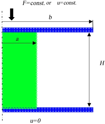
is the stress growth exponent. The accuracy and effectiveness of the Papanastasiou model in modeling of Bingham fluid flows has been demonstrated recently by Burgos et al. [24] using analytic solutions for antiplane flow in a corner [25]. The axisymmetric sample is shown in Figure 1. In this figure, H, a and b are the sample height, the wide of sample and the plate, respectively. Due to the symmetry of the sample, the compression test was simulated only for one half of the rectangular sample for two different cases when only the upper plate is moving with either constant velocity or under a constant force.

Figure 1. Geometry and boundary condition of the sample

The following scaled variables were used to represent the governing equation in the normalized form:

* * *

0

* *

0 0

, , ,

, ,

x u

x u

H U

t p

t p

H U

r r

r t t

t t

*

= = =

= = =

(6)

One needs to notice that in the case of constant load simulation, U is an arbitrary velocity and the load is scaled by 2

0H

t . Dimensionless forms of the governing

equations are:

0 1

= * × Ñ + *

* * D_Dt u

r

r (7)

* × Ñ * + * Ñ * -= *

*

t r r

1 1

Re p

Dt Du

(8)

* ú ú ú

û ù

ê ê ê

ë é

+ *

÷ ø ö ç è æ_- *

-=

* _g

g g

t &

& &

1 exp

1 M

Bn (9)

In the above equations, the dimensionless growth exponent is

H mU

M= . Reynolds and the Bingham

number are also defined as follows:

0 0

Re UH and Bn H

U

r t

m m

= = ₍₁₀₎

M should be sufficiently high so that the regularized Papanastasiou model provides a good approximation of the ideal discontinuous Bingham model. On the other hand, very high values of M are undesirable since they lead to convergence difficulties. In our study, the numerical results for M= 100 and 800 are essentially the same. Having the values of Re and Bn parameters in mind, in the present paper we have chosen the value 800 for M.

3. SMOOTHED PARTICLE HYDRODYNAMICS

In the SPH method, the fluid is represented by particles which are assumed to have fixed mass, and follow the fluid motion. The equations governing the evolution of the fluid become expressions for interparticle forces and flux when written in the SPH form [26]. The SPH theory is based on the idea that the smoothed representation A_s

( )

r of the continuous function A

( )

r at the position r can be found from:

( )

r A

( ) (

r W r r h

)

dr

A_s =

ò

¢ - ¢, ¢ (11)

where, h is the support scale of the weighted function

W. This function satisfied the following properties:

H

u=0

F=const.or u= const.

a

(

)

(

)

(

)

0

, 1,

li m ,

h

W r r h d r

W r r h d r r

® ¢ ¢ - = ¢ ¢ - =

-ò

(12)

For the numerical simulations, the fluid is represented by a discrete set of N particles. Therefore, the properties of the ith particle are calculated by approximating the integral (11) to the following summation:

( )

r m AW

(

r r h

)

A N _{j j}

j j j s , 1 -=

å

= r (13)

where, the summation is over N neighboring particles around the specified particle and mj,rj, rj are the mass, local density and position of the jth particle, respectively. The weighting function is a function of the relative distance r and h, (h being the corresponding smoothing length). Several forms have been proposed for the weighting function including the quintic spline which suggested by Morris for its high precision and stability [15]. It takes the following form:

(

)

( ) ( ) ( )

( ) ( )

( )

5 5 5

5 5

5

7 ,

478

3 6 2 15 1 , 0 1

3 6 2 , 1 2

3 , 2 3

0, 3

i j

W r r h

s s s s

s s s

s s s p - = - - - + - £ £ - - - £ £ - £ £ ³ ´ ì ï ï í ï ï î (14)

where, s is

h r r_i- _j

, when W is normalized for two

dimensions. Such a choice is also in good agreement with our results. The gradient of a typical function A is calculated via the formula:

÷ ø ö ç è æ -Ñ å =

Ñ _{j j}W r_i r_j h j j A j m i A , r (15)

but the form:

ij i j j j i i j i W p p m

A _÷÷Ñ

ø ö ç ç è æ + = ÷÷ ø ö çç è æ _Ñ

å

2 2

1

r r

r (16)

has been widely used as it conserves both linear and angular momentum exactly.

The second derivative of kernel function is very sensitive to particle disorder and can easily lead to numerical instability. Thus, the following form of the Laplacian of a function A is used in our simulation:

(

)

å

₊ ×₊Ñ

= ÷÷ ø ö çç è æ Ñ × Ñ j ij ij i ij ij j i j i r W r A m A 2 2 2 8 1 h r r r (17)

where, h is a small number with the value 0.1h and is inserted in the formula to avoid singularity.

4. SOLUTION PROCEDURE

The prediction-correction algorithm employed by Hosseini et al. [17] was used in the numerical algorithm. In this algorithm, the force terms of the right hand side of the momentum equation namely: body force, gradient of pressure, and the viscous force along with continuity equation are calculated in three distinct steps. In the first step, the momentum equation is solved in the presence of body force while neglecting other forces. The computed provisional velocity field is used as a primary prediction for the subsequent steps. However, in our study, the first step is not performed due to absence of gravity. In the second step (also known as a prediction step) the calculated velocities at previous time step is used to compute the rate of strain tensor component (_g&=Ñu+

( )

_ÑuT_{) followed by the computation of the}

corresponding divergence. Unlike the Hosseini's formulation, here the viscous term derived by Morris [15] was utilized in our simulations:

(

)

å

_÷÷

ø ö ç ç è æ ¶ ¶ + = þ ý ü î í ì ÷÷ ø ö çç è æ Ñ × Ñ j i ij ij j i ij j i j i r W r u m u 1 1 r r m m m r (18)

where, the fluid viscosity was replaced by the apparent viscosity from regularized Papanastasiou relation as follows:

(

)

1 exp 1 app app M Bn g

t m g m

g

*

* *

*

é _{- -} ù

ê ú = ® = + ê ú ë û & & & (19)

The Bingham plastic behavior is exerted by this apparent viscosity thereby the second part of right hand side of Equation (2) is calculated. At the end of the second step, the velocity components is updated, and the intermediate positions are obtained.

In the third step of the algorithm, i.e. the corrector step primarily, the density changes due to the temporary position and velocity update of the particles was calculated using the continuity equation:

(

)

( )

å

- ×Ñ

= j ij i j i j

i _{m u u Wr h} Dt

D

, r

(20)

Pressure of each particle can be obtained through the combination of Equation (21) and Equation (17) and the following form of Equation (21) is obtained:

(

)

0

2 2 2 2

0

8 j ij i ij i

i

j _{i ij}

j

P x W

mj P

t _r

r r

r r r h

× Ñ

-= + +

D _{+ +}

æ ö

ç ÷

ç ÷

ç ÷

è

å

ø

(

)

2 2 ₂

8 j ij i ij

j _ij

i j

P x W

mj r h r r × Ñ + + + æ ö ç ÷ ç ÷ ç ÷

è

å

ø

(22)

The final velocity of this step is then calculated and the new position of each particle is obtained:

(

t t

)

i t i t t i t

i u u

t x

x ₌ +D ₊D ₊ +D

2 (23)

4. 1. Force Calculation The most common SPH approximation of the momentum equation is:

÷ ø ö ç è æ -Ñ

å ÷ø

ö ç è æ -÷ ø ö ç è æ ₊

å Ñ ç_èæ - ÷_øö+ ÷ ÷ ÷ ø ö ç ç ç è æ + -= h j r i r W i

j i j

j u i u j i j m j h j r ir W i i i P j j P j m dt i du , , 2 2 r r m m r r (24)

In order to obtain the modified SPH model, the change of momentum for ith particle with a constant mass can be written as:

i i

i f

dt du

m = (25)

where, f_i is the total force acting on the particle i. By observing the point force relation in Equation (25) and the SPH equation i.e. Equation (24), the SPH approximation of the force acting on a particle due to momentum conservation is shown in the following equation:

(

)

(

)(

) (

)

h r r W u u m m h r r W P P m m f j i i

j i j

j i j i j i

j i i i j

i j j j i i , , 2 2 -Ñ -+ + -Ñ ÷ ÷ ø ö ç ç è æ + -=

å

å

r r m m r r (26)

In the case of constant velocity, the effective load at the top side of the sample for each particle is calculated using Equation (25).

4. 2. Boundary and Initial Conditions The initial velocity and the initial pressure are set to zero for all the particles. The boundary conditions imposed on the simulation domain are shown in Figure 1. In the current study, the mass between two plates is constant, 2a=H

and the lower plate is fixed whereas the upper one is moving. In the case of a constant velocity, the

transverse non-dimensional velocity is set to -1 (the minus sign indicates that the velocity is in the direction of the compression of the sample); while, the boundary condition for the case of the constant load will be discussed in the following section.

4. 2. 1. Constant Load Condition There is a relationship between the force field acting on the particle and the force acting on a particle i:

dt du m f F _i i i i i _{= =}

r (27)

Therefore, the Navier- Strokes equation is formulated in the general form as follows:

i i i i i m f P dt du + × Ñ + Ñ -= r t r (28)

The third term on the right hand side of the above equation is valid only for the wall particles to exert the constant load condition.

4. 2. 2. No-slip Condition In order to accurately model the compression of the sample, the no-slip boundary condition needs to be applied on the walls. Although several methods have been introduced to model the rigid boundaries in SPH, these boundaries in our simulations were assumed to be filled with fixed (or moving but with a prescribed velocity) particles and the fluid solution algorithm was partially applied to these boundary particles.

This procedure includes only the solution of the third step of the solution algorithm (considering the prescribed movement of the rigid walls for moving rigid boundaries) to repulse the inner flow particles accumulating in the vicinity of the wall. Therefore, the pressure of the wall particles increases due to increasing of particle density near the rigid wall thereby the inner fluid particles are repelled from the wall, and vice versa. Velocities of the wall particles were set to zero at end of each time step to simulate a fixed wall. This velocity for moving walls are known and the movement of this particle is based on this known velocity.

No-slip boundary condition was required at the interface of fluid and the wall. This condition has been implemented using an imaginary velocity for the wall particles. Figure 2 illustrates the concept for a curved boundary. For each particle of fluid, e.g. particle a, and boundary particles B, the normal distance to the boundary was calculated. Then, the velocity of particle

Figure 2. No-slip boundary condition

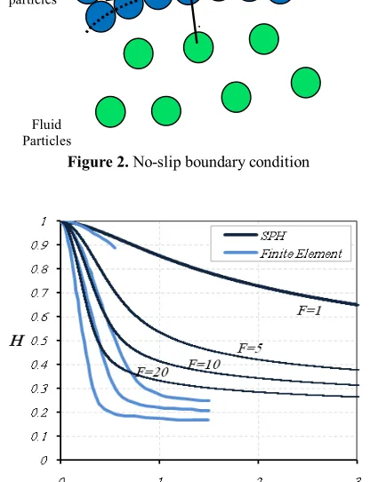
Figure 3. Change of sample's height, for Re= 10 and Bn= 0.5

5. NUMERICAL RESULTS

In order to assess the ability and the efficiency of the SPH algorithm, it was tested against the simulation of a squeeze flow with different flow regimes and boundary conditions. In the case of dynamic yield stress measurements, evaluation of the final height is sufficient considering constant load. However, it is yet an open question which occurs below or closed to the yield stress.

The simulations were obtained for the constant load and constant velocity conditions, for a rectangular sample. The results were reported for different Reynolds and Bingham numbers as well as different exerted load on the wall. Since no experimental results exist based on the aforementioned condition, the results were compared with the results of the finite element method for a cylindrical sample, which in two-dimensions represents the rectangular geometry of the current 2D simulations.

In the current simulation, non-zero Reynolds number, constant mass between the plates, b>a, and

2a=H were considered. The lower plate was fixed and the upper one was moving with a constant velocity or under a constant load. Change of the sample’s height

and load on the wall particles were calculated during the compression of the sample for different Reynolds and Bingham numbers. Shape of the sample and its squeezed form were illustrated under the constant load condition.

5. 1. Constant Load In the constant load condition, the change of sample's height was calculated for various Bingham numbers and different values of exerted loads during the process. Figure 3 shows the compression rate for different values of exerted loads while Re=10 and

Bn=0.5. The behavior of deformation for both SPH and Finite Element methods is similar. The rate of compression increases with increasing the constant load. The notable difference was the higher rate of deformation for the sample modeled by Finite Element Method which might be caused due to the difference in the method of applying load on the sample. In the SPH approach, the force was exerted on the particles of the upper wall and thereby on the fluid particles. However, the force was directly applied on the upper elements of fluid in Finite Element simulations. The aforementioned deference besides the error arisen due to interpolation, led to the damped results. Moreover, in the Finite Element simulations the plate stops in a finite time and its velocity decreases very rapidly. On the contrary with the results reported in references [4], in the case of F=-1 the deformation did not stop and continued slightly. In the Papanastasiou model, where all materials are modeled as a liquid with an arbitrary large viscosity, the elements of _g* _{matrix did not entirely vanish even}

when the stresses were below of yield limit and the deformation continues slowly because of the increase in the artificial viscosity.

Figure 4 illustrates the SPH results in comparison with the finite element results of Florides et al. [4].The test was performed for Bingham numbers, 1, 4 and 5 at

F=-10 as well as Re=1. In order to study the effect of Bingham number, the dimensionless force was chosen asF*=F´Bn_{. Figure 4 indicates a similar behavior in}

both approaches, i.e. the artificial viscosity and the resistance of the fluid increase with increasing in Bingham number and consequently the upper plate stops at a farther distance from the lower one. Different rate of compression was observed between the SPH method and the Finite Element Method in this case. This might be due to the different nature of two methods; meaning that the interpolation function of the SPH approach produces ahigher order smooth interpolation field in all dimensions. The effect of variation in Bingham number in the overall results was more evident in SPH method. As mentioned before, the compression did not stop and continued slightly until the exit of all material from the space between the plates. Since the artificial viscosity increased, the deformation rate of the sample declined. In addition, one should notice that

Wall particles

Tangentia l

B

d

d

another source of error in Finite element method occurs as a result of remeshing procedure whereas in the SPH methodology, the meshfree nature could lead to high ability in modeling of such high deformations.

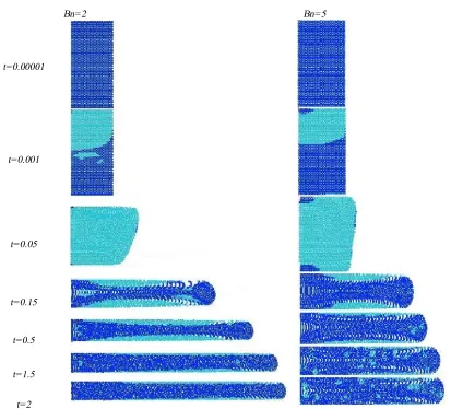
The snapshots of the sample during the time evolution were plotted in Figure 5 for Bn=2 and Bn=5,

Re=1 and F=-10. Initially, in agreement with those reprted by Florides et al. [4], the growth of the yielded regions led to deformation of the sample and only a small unyielded region remained in the plate center. As the deformation increased, the growth of this initially small region led to reduction of the deformation rate. Nevertheless, there always exist unyielded regions far from the center of the plates that keep a permanent deformation going. The growth of unyielded region (dark blue) increased with the increase of Bingham

number. Figure 4.. Change of sample's height, for Re= 1 and F=-10.

Bn= 2 Bn= 5

t=0.00001

t=0.001

t=0.05

t=0.15

t=0.5

t=1.5

t=2

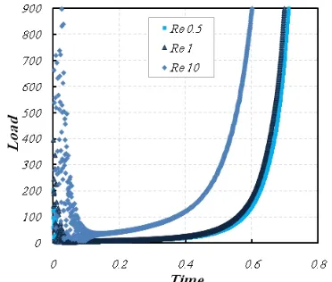
5. 2. Constant Velocity In a squeeze flow test under constant velocity, the force required to keep constant the velocity of the upper disk is of great importance. This load was calculated using Equation (26) over the nearest fluid particles to the top wall. The variations of resultant load on the top side of the sample with various Reynolds numbers are shown in Figure 6. Moreover, Figure 7, illustrates calculated load with different Bingham numbers. These figures show that the exerted load on the wall increases in the same behavior with previous works. The overall behavior of the samples simulated with SPH method is similar to other currently used methodologies.

Nevertheless, the obtained numerical values are slightly different. Figure 6 reveals three regions with different behaviors. In the primary part, we observe that the Curve descends from a large value, the physical infinity, to a rather small value. The dimensionless time for the force to approach a finite steady state was reported about 0.06 in [4]. This value was 0.01 in the results reported in this paper for Re=1. In fact, imposing a sudden constant velocity on the upper surface in the initial times is one of the main factors that delay the steady state. The instantaneous imposing of the constant velocity condition on the upper surface resembles the collision of two bodies where the momentum of the wall is not affected by that of the fluid. Of course, this is a rather idealistic condition than what actually occurs in reality.

Consequently, as a very high pressure is produced between the fluid and the surface of the plate, the fluid velocity exceeds that of the surface and a negative relative pressure between the two bodies creates. When this pressure wave propagated through the sample, before its deformation, we observed the pressure fluctuations in the boundary of the two bodies and the upper wall. In reality, there is a consequent force fluctuation. The Finite Element Method, especially in higher Reynolds’s numbers, cannot capture the aforementioned state, and as a result, higher values were reported for the time required to reach a steady state in the previous studies.

In the intermediate section, as the oscillations started damping in the beginning of the condensation process, a descending diagram with a moderate change was observed. In the ending step, as the plate came down and more changes occurred in the form of the sample, more particles were affected by the plate.Consequently, the exerted force on the plate increased which was in good agreement with the finite element results. Furthermore, increasing deformation in the ending part led to sudden increase in the force.

In the mesh base methods, the aspect ratio is the measure of the stretching of the cells. A general rule of thumb is to avoid aspect ratios that exceed 5:1. The Finite Element simulation fails to march above a critical time, as the sample becomes very thin and the surface of

the sample very large, hence high aspect ratio of elements. Such a problem does not arise in the SPH methodology. Although there is not experimental data on the ending steps to make a comparison between methods of FEM and SPH, the above reasoning might lead us to the conclusion that SPH is more versatile than FEM for high deformation of the materials.

Meanwhile, in SPH approach, including in the present study, no smoothing is used while in Finite Element method, because of pressure fluctuations arisen due to the discontinued motion of nodes, the relatively cumbersome smoothing is inevitable.

Figure 6. Resultant load at the top side, for Bn= 0.5 and v=-1

6. CONCLUSION

The main aim of this work was to evaluate a particle method for the simulation of large deformation of a squeezed material because of their simplicity in application, time saving, and programming. The three-step SPH, which guaranties the incompressibility constraint, was chosen and applied to the deformation of squeezed materials during their large deformations in two different loading boundary conditions.

Results were compared with those previously obtained by Finite Element Method for both boundary conditions. Although both methods represented the same behavior, their results differed in some aspects. This might be due to the fact that no remeshing occurs in SPH method because of its ability in simulation of large deformations. In addition, because of its meshfree nature and assumption of wall particles, load and velocity boundary conditions are not directly applied to the fluid particles which are closer to the real test. The aforementioned reasons, besides its higher order interpolation function, lead to a successful application of Bingham formula within the SPH methodology. Consequently, the deformations are considerably smoother. These facts candid the presented SPH method as a fast and simple method for future studies of viscoplastic materials.

7. REFERENCES

1. Bird, R. B., Dai, G. and Yarusso, B. J., "The rheology and flow of viscoplastic materials", Reviews in Chemical Engineering, Vol. 1, No. 1, (1983), 1-70.

2. Sherwood, J. and Durban, D., "Squeeze-flow of a Herschel–

Bulkley fluid", Journal of Non-newtonian Fluid Mechanics, Vol. 77, No. 1, (1998), 115-121.

3. Adams, M., Aydin, I., Briscoe, B. and Sinha, S., "A finite element analysis of the squeeze flow of an elasto-viscoplastic paste material", Journal of Non-newtonian Fluid Mechanics, Vol. 71, No. 1-2, (1997), 41-57.

4. Florides, G. C., Alexandrou, A. N. and Georgiou, G. C., "Flow development in compression of a finite amount of a Bingham plastic", Journal of Non-newtonian Fluid Mechanics, Vol. 143, No. 1, (2007), 38-47.

5. Dean, E. J., Glowinski, R. and Guidoboni, G., "On the numerical simulation of Bingham visco-plastic flow: Old and new results",

Journal of Non-newtonian Fluid Mechanics, Vol. 142, No. 1, (2007), 36-62.

6. Smyrnaios, D. and Tsamopoulos, J., "Squeeze flow of Bingham plastics", Journal of non-newtonian fluid mechanics, Vol. 100, No. 1, (2001), 165-189.

7. Karapetsas, G. and Tsamopoulos, J., "Transient squeeze flow of viscoplastic materials", Journal of Non-newtonian Fluid Mechanics, Vol. 133, No. 1, (2006), 35-56.

8. Liu, G. R. and Liu, M., "Smoothed particle hydrodynamics: a meshfree particle method", World Scientific Publishing Company Incorporated, (2003).

9. Lucy, L. B., "A numerical approach to the testing of the fission hypothesis", The Astronomical Journal, Vol. 82, No., (1977), 1013-1024.

10. Gingold, R. A. and Monaghan, J. J., "Smoothed particle hydrodynamics-theory and application to non-spherical stars",

Monthly Notices of the Royal Astronomical Society, Vol. 181, (1977), 375-389.

11. Monaghan, J. J., "Why particle methods work", SIAM Journal on Scientific and Statistical Computing, Vol. 3, No. 4, (1982), 422-433.

12. Monaghan, J. J., "An introduction to SPH", Computer Physics Communications, Vol. 48, No. 1, (1988), 89-96.

13. Shao, S. and Lo, E. Y. M., "Incompressible SPH method for simulating Newtonian and non-Newtonian flows with a free surface", Advances in Water Resources, Vol. 26, No. 7, (2003), 787-800.

14. Ellero, M., Kröger, M. and Hess, S., "Viscoelastic flows studied by smoothed particle dynamics", Journal of Non-newtonian Fluid Mechanics, Vol. 105, No. 1, (2002), 35-51.

15. Morris, J. P., Fox, P. J. and Zhu, Y., "Modeling low Reynolds number incompressible flows using SPH", Journal of Computational Physics, Vol. 136, No. 1, (1997), 214-226. 16. Rafiee, A., Manzari, M. and Hosseini, M., "An incompressible

SPH method for simulation of unsteady viscoelastic free-surface flows", International Journal of Non-Linear Mechanics, Vol. 42, No. 10, (2007), 1210-1223.

17. Hosseini, S., Manzari, M. and Hannani, S., "A fully explicit three-step SPH algorithm for simulation of non-Newtonian fluid flow", International Journal of Numerical Methods for Heat & Fluid Flow, Vol. 17, No. 7, (2007), 715-735.

18. Jun, S., Liu, W. K. and Belytschko, T., "Explicit reproducing kernel particle methods for large deformation problems",

International Journal for Numerical Methods in Engineering, Vol. 41, No. 1, (1998), 137-166.

19. Calvo, B., Martinez, M. and Doblare, M., "On solving large strain hyperelastic problems with the natural element method",

International Journal for Numerical Methods in Engineering, Vol. 62, No. 2, (2005), 159-185.

20. Bingham, E. C., "Fluidity and plasticity", McGraw-Hill, (1922). 21. O'Donovan, E. and Tanner, R., "Numerical study of the Bingham squeeze film problem", Journal of Non-newtonian Fluid Mechanics, Vol. 15, No. 1, (1984), 75-83.

22. Mitsoulis, E., Abdali, S. and Markatos, N., "Flow simulation of herschel‐bulkley fluids through extrusion dies", The Canadian Journal of Chemical Engineering, Vol. 71, No. 1, (1993), 147-160.

23. Papanastasiou, T. C., "Flows of materials with yield", Journal of Rheology, Vol. 31, No. 5, (1987), 385-404.

24. Burgos, G. R., Alexandrou, A. N. and Entov, V., "On the determination of yield surfaces in Herschel–Bulkley fluids",

Journal of Rheology, Vol. 43, No. 3, (1999), 463-483. 25. Rigaut, C., Janin, B., Laty, P., Bourg, A. and Latrobe, A.,

"SIMULOR: un logiciel de modélisation 3D du remplissage et de la solidification en moulage", Hommes et Fonderie, No. 193, (1989), 13-24.

Numerical Simulation of Squeezed Flow of a Viscoplastic Material by a Three-step

Smoothed Particle Hydrodynamics Method

P. Ghalandari, N. Amanifard, K. Javaherdeh, A. Darvizeh

Mechanical Engineering Department, Faculty of Engineering, University of Guilan, P.O. Box 3756, Rasht, Iran

P A P E R I N F O

Paper history:

Received 27 May 2012

Accepted in revised form 18 October 2012

Keywords: SPH

Meshless Method Viscoplastic Materials Squeeze Flow

هﺪﯿﮑﭼ

ﻪﮑﺒﺷنوﺪﺑيدﺪﻋشورﮏﯾﻪﻟﺎﻘﻣﻦﯾارد SPH

ﺘﺳﻼﭘﻮﮑﺴﯾوداﻮﻣيارﺬﮔرﺎﺘﻓرﯽﺳرﺮﺑﺖﻬﺟ ﺖﺳاهﺪﺷﻪﺘﻓﺮﮔرﺎﮐﻪﺑﮏﯿ

.

ﻪﺑﺎﺑ ﻪﯿﺒﺷشورﻦﯾايﺮﯿﮔرﺎﮐ ﺪﺷمﺎﺠﻧاﻪﮑﺒﺷﺪﯿﻟﻮﺗراﻮﺷدﺪﻨﯾآﺮﻓنوﺪﺑنآدازآﺢﻄﺳوﻪﻧﻮﻤﻧگرﺰﺑﻞﮑﺷﺮﯿﯿﻐﺗيزﺎﺳ

.

ﻦﯾا

شور SPH ﻪﻠﺣﺮﻣﻪﺳ ﻮﮕﺸﯿﭘﺢﯾﺮﺻﮏﯿﻨﮑﺗﮏﯾيا

-حﻼﺻا ﻪﺑارهﺪﻨﻨﮐ ﯽﻣرﺎﮐ ندﻮﺑﻢﮐاﺮﺗﻞﺑﺎﻗﺮﯿﻏﻪﺼﺨﺸﻣﻆﻔﺣودﺮﯿﮔ

ﺎﻌﻣﮏﯾﻞﺣﺎﺑارداﻮﻣ ﯽﻣﻦﯿﻤﻀﺗنﻮﺳآﻮﭘرﺎﺸﻓﻪﻟد

ﺪﻨﮐ

.

ﻪﯿﺒﺷﻦﯾاردﻦﯿﻨﭽﻤﻫ ،يزﺎـﺳ

يرﺎﺘﺧﺎـﺳلﺪـﻣ Papanastasiou

ﺛﺖﻋﺮﺳوﺖﺑﺎﺛيوﺮﯿﻧيزﺮﻣطﺮﺷودﺖﺤﺗﻪﻧﻮﻤﻧﻞﮑﺷﺮﯿﯿﻐﺗﻪﻌﻟﺎﻄﻣﺖﻬﺟ ﺖـﺳاﻪﺘﻓﺮﮔراﺮﻗهدﺎﻔﺘﺳادرﻮﻣﺖﺑﺎ

.

طﺮـﺷ

ﺖﺳاهﺪﺷلﺎﻤﻋاﯽﺑﻮﺧﻪﺑهراﻮﯾدتارذيورﺮﺑﮏﯿﺘﺳﻼﭘﻮﮑﺴﯾوداﻮﻣﺖﻋﺮﺳندﺮﮐﺮﯾﻮﺼﺗﺎﺑشﺰﻐﻟمﺪﻋيزﺮﻣ

.

رﻮﻈﻨﻣﻪﺑ

،ﻪﻧﻮﻤﻧﻢﮐاﺮﺗﺪﻨﯾآﺮﻓﯽﻃرديدﺪﻋشورﻦﯾاﯽﺘﺳردﻖﯾﺪﺼﺗ

ﻦﯿـﻨﭽﻤﻫوﺖﺑﺎﺛﺖﻋﺮﺳيزﺮﻣطﺮﺷردهﺪﺷلﺎﻤﻋايوﺮﯿﻧ

ﻪﻧﻮﻤﻧعﺎﻔﺗراﺮﯿﯿﻐﺗ هﺪﺷﻪﺴﯾﺎﻘﻣﺮﮕﯾدﻪﺑﺎﺸﻣﺞﯾﺎﺘﻧﺎﺑوهﺪﺷﻪﺒﺳﺎﺤﻣﺖﺑﺎﺛوﺮﯿﻧيزﺮﻣطﺮﺷرد

ﺪﻧا

. ﺐـﻠﻄﻣﻦﯾايﺎﯾﻮﮔﺞﯾﺎﺘﻧ

ﻪﯿﺒﺷردنﺎﻨﯿﻤﻃاﻞﺑﺎﻗشورﮏﯾناﻮﻨﻋﻪﺑﺪﻧاﻮﺗﯽﻣشورﻦﯾاﻪﮐﺖﺳا

ﻞﮑـﺷﺮﯿﯿﻐﺗﺖﺤﺗﻪﮐﮏﯿﺘﺳﻼﭘﻮﮑﺴﯾوداﻮﻣيزﺎﺳ

ﯽﻣراﺮﻗدﺎﯾز ،ﺪﻧﺮﯿﮔ

ﻪﺑ دوررﺎﮐ

.