Leaf shape simulation of castor bean and its application in nondestructive leaf area estimation

Leaf shape simulation of castor bean and its application in nondestructive

leaf area estimation

Hailin Wei

,

Xumeng Li

,

Ming Li

,

Huang Huang

2. Hunan Academy of Forestry, Changsha 410004, China; 3. Hunan Academy of Agricultural Sciences, Changsha 410000, China)

Abstract: The leaf shape and leaf area measurement are crucial in plant growth modeling. The castor bean leaf is large, palm-shaped with multiple clefts. The leaf shape simulation and leaf area estimation were less studied. The circular model and nonrectangular hyperbolic model were developed to describe the standard leaf shape of castor bean in this study, providing a model for simulating the leaf shape and a nondestructive way for estimating the leaf area respectively. In addition, a formula was established to estimate the leaf area by the parameter of the standard leaf shape of castor bean. Based on validation results, the circular model fits the landmarks and nonrectangular hyperbolic model fits the lobe margins very well. The leaf area was accurately estimated by using the established formula. This study could provide a theoretical reference for leaf visualization, a nondestructive and easy way to estimate the leaf area for other complex leaves with multiple lobes.

Keywords: leaf shape, leaf area, geometrical characteristics, mathematical model, image processing, plant growth modeling DOI: 10.25165/j.ijabe.20191204.4040

Citation: Wei H L, Li X M, Li M, Huang H. Leaf shape simulation of castor bean and its application in nondestructive leaf area estimation. Int J Agric & Biol Eng, 2019; 12(4): 135–140.

1 Introduction

The leaf is an important organ of plants. Plant leaves participate in many physiological processes, such as transpiration, photosynthesis and so on. The leaf area is an important determinant of light interception and consequently of transpiration, photosynthesis and plant productivity[1]_{. Thompson}[2] _{stated that} the area of an object was proportional to the square of its length (the area-length allometry). O’Shea et al.[3] _{studied the allometric} relationship between the surface and the length of six species of fish. The estimates of the exponent of the first allometry ranged from 1.88 to 2.22. Montgomery[4] _{put forward a leaf area formula} for corn: the leaf area (A)=k×leaf length (L)×leaf width (W). Where k is a constant to be fitted; The leaf length is defined as the distance from leaf apex to leaf base; The leaf width is defined as the maximum length of the segments perpendicular to the straight line passing through leaf apex and leaf base[5]_{. The Montgomery} model has been demonstrated to be appropriate for calculating leaf area for other herbaceous and woody plants such as cotton, rice and sorghum[6-8]_{. These models would have many advantages, such as} an expression in dimensional terms of length and width of a leaf, which would be easy to measure many plants with simple shape leaf, but not to easy measure other plants with complex shape leaf, such as caster bean leaf.

Recently, many studies have proposed parametric models to describe leaf shapes of some plants. These models can be used to calculate leaf area. For instance, Shi et al.[9] _{used the elliptical}

Received date: 2018-12-10 Accepted date: 2019-05-13

Biographies: Hailin Wei, PhD, Senior Engineer, research interests: crop

information science and digital forestry, Email:[email protected]; Xumeng Li, PhD, Associate Professor, research interests: crop information science, Email: [email protected]; Ming Li, PhD, Professor, research interests: crop

information science, Email: [email protected].

*Corresponding author: Huang Huang, PhD, Professor, research interests:

crop information science. Hunan Agricultural University, Changsha 410128, China. Tel: +86-13548583644, Email: [email protected]; xh.wang@ hunau.edu.cn.

equation, the sectorial equation and the simplified Gielis equation to describe the leaves of Hydrocotyle vulgaris, Ginkgo biloba L.,

Polygonum perfoliatum L. and Oligostachyum sulcatum, and used these mathematical equations to derive the theoretical value of the Montgomery parameter. Dornbusch et al.[10] _{put forward a} general parameter model to depict the leaf shapes of wheat, barley and maize. Gielis[11] _{proposed a superformula that could be used} to describe the shapes of many abiotic and biotic objects, which has been simplified to fit to leaf dimensions. The simplified Gielis equation (SGE) has only two parameters. One is related to leaf length, and the other is related to the ratio of leaf width to length. Shi et al.[12,13] _{used the SGE to fit the leaf shapes of plants such as}

Indocalamus sp., Aucuba japonica var. variegata Dombrain,

Chimonanthus praecox (L.) Link, Parrotia subaequalis (H. T. Chang) R. M. Hao & H. T. Wei, Phoebe sheareri (Hemsl.) Gamble and Pittosporum tobira (Thunberg) W. T. Aiton. However, these mathematical models would be not appropriate for complex caster bean leaf.

Castor bean (Ricinuscommunis L.) belongs to the family

Euphorbiaceae and the genus Ricinus. Although, the castor bean was planted at the industrial scale in more than 30 countries, the leaf shape simulation and LA estimation were less studied. Jani and Misra[14] _{stated Montgomery model to estimate the area of} Castor bean leaf, however, it would be not easy to know well the measure of the length and width of the leaf with different number of clefts. The castor bean leaf is large, palm-shaped with multiple clefts, which would not be described well by above mathematical model. In this study, a simulation model was constructed to describe geometric shape of castor bean leaf, and a formula of leaf area was derived by the model parameters. In addition, this model would be applied in the visualization of castor bean leaf and the identification of castor bean.

2 Materials and methods

2.1 Plant materials and leaf description

located in a subtropical monsoon humid climatic zone (28.25°N, 113.41°W; the elevation is 65 m; the mean annual temperature is 17°C; the mean annual precipitation is 1400 mm). The soil in the garden is red-yellow mud paddy soil developed from Quaternary red clay. The contents of soil organic matter, total nitrogen, total phosphorus, total potassium, available nitrogen, available phosphorus and available potassium were 33.51 g/kg, 1.52 g/kg, 0.94 g/kg, 12.68 g/kg, 130.12 mg/kg, 30.78 mg/kg and 134.71 mg/kg respectively. Four varieties of castor beans were planted on the ridges of the garden with row spacing and plant spacing of 0.8 m which is the recommended planting density. 300 kg/hm2 _{phosphorus diamine was used as a basal} fertilizer in total during the plowing (i.e., before the planting). Based on the soil moisture content, the irrigation was used to prevent the plants from experiencing drought stress, and the weeding was performed regularly.

For convenience, the geometric parameters determined in the

study are shown in Figure 1.

In Figure 1, αi is the intersection angle between adjacent leaf veins; βi is the intersection angle between adjacent leaf veins and leaf valley lines. The serial numbers refer to leaves counterclockwise from the main leaf vein. The leaf edge (green line) is the entire boundary of the leaf. The longest vein was denoted by blue line, and the joint point of all veins was denoted by the leaf center (blue dot). The leaf apexes (red dots) are determined from the joint point of the leaf vein and the leaf edge where N is the number of lobes. The leaf valley endpoint (yellow dots) is the dividing point of the lobes which is the nearest point from the lobe margin to the leaf center. The vein lines (pink lines) are drawn from the leaf apexes to the center. These lines are usually referred to as veins. The leaf valley lines (blue dashed lines) connect the leaf valley endpoints to the center. The lobe margin refers to the leaf boundary connecting a leaf apex and a leaf valley endpoint. Thus, each lobe has two edges.

a. Description of the term used in this study b. Description of the circular models for leaf apex and leaf valley endpoints

c. Description of the coordinate frame for the lobe margin model

Figure 1 Description of Ricinuscommunis L. leaf used in this study 2.2 Sample collection and data processing

2.2.1 Sample collection

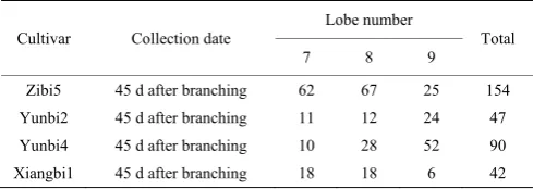
Leaves were sampled randomly 45 d after branching in 2018. The samples include 333 leaves of four varieties (Zibi5, Yunbi2, Yunbi4, and Xiangbi1). Two hundred leaves were classified into 18 sample groups by variety and lobe number (Zibi5:6-11 lobes, Yunbi2:6-9 lobes, Yunbi4:7-10 lobes and Xiangbi1:6-9 lobes). As some groups (Zibi5:6 and 11 lobes, Yunbi2:6 lobes, Yunbi4:10 lobes, and Xiangbi1:6 lobes) had few leaves, 12 sample groups (four varieties: Zibi5, Yunbi2, Yunbi4, and Xiangbi1; three numbers of lobes: 7-9) were used in this study. In Table 1 the sample information was shown. Photos of samples can be found in the supplementary information (S1_Data). The sample group Zibi5 was used for the model development, discussion and application, and others were used for discussion and application partly.

Table 1 Lobe Numbers of sample leaves

Cultivar Collection date

Lobe number

Total 7 8 9 Zibi5 45 d after branching 62 67 25 154 Yunbi2 45 d after branching 11 12 24 47 Yunbi4 45 d after branching 10 28 52 90 Xiangbi1 45 d after branching 18 18 6 42 2.2.2 Data processing

Samples were pressed and photographed against a background

(1280×1024 pixel resolution) with the instrument described[15]_. Leaf binary images were obtained after differential operation of the image and background. The leaf edge was extracted by using the boundary-tracking algorithm[16]_{. And the additional geometric} parameters, such as leaf apexes and valley endpoints, edges of lobes and leaf area (LA), were extracted based on the leaf edge. The detailed steps are as follows:

Step 1. Pixel coordinates of the leaf center were marked manually.

Step 2. Differential operation of the image and background[17] was carried out by using Equation (1), and the result was recorded as LIMd where LIM and BIM indicate the RGB data[18] _{of the leaf} image and background respectively.

LIMd(i, j, k)=LIM(i, j, k)–BIM(i, j, k) (1) When k=1, 2,3, the values of LIM(i, j, k) and BIM(i, j, k) are the red, green and blue channels of the leaf image and background at pixel (i, j) respectively.

The image binar ization was performed by using Equation (2): 1 ( , ,2)

( , )

0 ( , ,2)

LIM i j TH LIMb i j

LIM i j TH

≥ ⎧

= ⎨ _<

⎩ (2) where, LIMb is the binarized image and TH is the threshold adjusted to obtain a high-quality binarized image.

of 3 pixels to smooth the leaf image.

Step 4. Leaf margin was obtained with boundary tracking[21]_. Then, the pixel coordinates of leaf apexes and valley endpoints were determined by finding peaks with a minimum separation of 45 pixels[22]_{. The edges of the lobe were separated by leaf apexes} and valley endpoints. After image holes were filled[23]_{, the leaf} pixel area was calculated.

Step 5. Pixel coordinates of the leaf center, landmarks and point on the leaf margin were transformed to standard coordinates in a real coordinate frame (standard coordinate frame). The coordinate frame was shifted to ensure that its origin was overlapped with the leaf center. It was also rotated to ensure that its x-axis was overlapped with the longest vein and its unit was normalized to the length of the longest vein by transformation, translation and scaling.

2.3 Models and validation

2.3.1 Circular curve for landmark distribution

The distribution of landmarks (leaf apexes and valley endpoints) determining the profile of leaves is an important factor affecting the area of a palm-shaped leaf. As the geometric characteristics of castor bean leaves were nearly circular (Figure 1b), the distribution of leaf apex and valley positions was simulated based on a circular curve (Equation (3)) as follows:

(x –x0)2 –(y –y0)2=r2 (3) where, (x0, y0) is the circular center; r is the radius.

2.3.2 Lobe margin model

The lobe margin model describing the curves of half of the lobe margin in the coordinate systems was demonstrated in Figure 1b. In this model, the distance of a point on the lobe margin to a leaf vein was defined as a function of the distance from the leaf apexes to the projection of the lobe margin point on the leaf vein (Figure 1b). A nonrectangular hyperbolic equation[24] _and modified logistic model[25] _{were used in this study (as shown in} Equations (4) and (5)).

(4)

0

0 ( )

( 1)

rl m

m rl

m

H H e

H l H

H H e

= −

+ − (5) In Equations (4) and (5), the l and H represent the length of the vector projected from the point to leaf apexes on the leaf vein and the distance of the point on the lobe margin from the leaf vein respectively. The light response curve of the photosynthetic rate was obtained by Equation (4) where , Hm, and θare the initial slope of the corresponding curvature, asymptotically final value and curvature respectively. Equation (5) was modified from a logistic model in which H0, Hm and r represent the initial value of the “S-type” curve, final value and parameter depicting the rate of the curve change respectively. The term –H0 is introduced to

ensure that the leaf apex is located above the veins, that is, H(0)=0. 2.3.3 Simulation of standard leaf shape

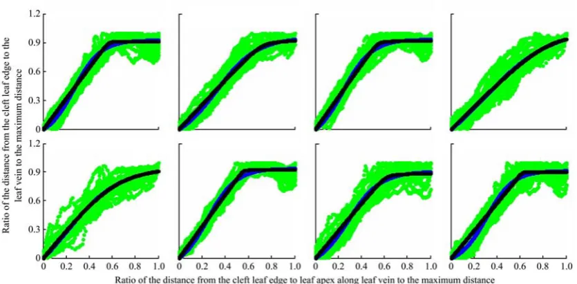
The parameters of each leaf in Equation (3) were obtained by fitting the coordinates of leaf apexes and valley endpoints, and the parameters of each leaf in Equations (4) and (5) were fitted based on the coordinates of the edges of each lobe. The standard leaf shape was simulated as follows: The landmark distribution was simulated by the circular model with the mean parameters and the mean angle between the adjacent leaf vein line and valley line (Table 2); Then, the lobe margin model was run by Equations (4) and (5) with the mean parameters. The result of standardized leaf simulation was shown in Figure 2.

Figure 2 Standardized shape of a blade with 7-9 lobes 2.3.4 Leaf area calculation

The area (S) of each standard leaf was calculated by integrating the polar coordinates. Thus, the LA was calculated by using Equation (6).

S=k×s×(r×L)2 ₍₆₎ where, L is the vein length; r is the radius of the leaf; s is the area of standard leaf and k is the regression coefficient of s×(r×L)2 _and actual leaf area.

2.3.5 Validation

The calculations in this study were carried out in MATLAB R2016a, and the performance of the model simulation was determined by the normalized root mean square error (RMSEn):

2 1

Σ ( ] 1

100%

n

i i

OBS SIM RMSEn

n OBS

−

= × × (7)

When the RMSEn value is less than 10%, two values are desirably consistent. When the RMSEn values are 10%-20%, 20%-30% and greater than 30%, a good simulation, an acceptable simulation and a poor simulation were indicated respectively[26]_.

3 Results and discussion

3.1 Parameters of landmark distribution

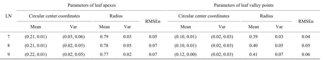
The parameters (circular center and radius) in Equation (3) were determined by fitting the standard coordinates of landmarks for each leaf with 7-9 lobes and using nonlinear regression[27]_. Based on the results (Table 2), the y-coordinates of the circular center of leaf apexes are small, i.e., the circular center is roughly located on the main leaf vein.

Table 2 Parameters of circles fitted for leaf apexes and leaf valley points

LN

Parameters of leaf apexes Parameters of leaf valley points Circular center coordinates Radius

RMSEn

Circular center coordinates Radius

RMSEn

Mean Var Mean Var Mean Var Mean Var

In addition, for the circle of leaf apexes, the x-coordinates of the circular center in the coordinate frame are 0.21, 0.21, and 0.22, respectively, and the radii are 0.79, 0.78, and 0.77 for 7-9 lobes respectively. In other words, the center of the circle moves slightly away from the leaf center and the ratio of the radius to the leaf length slightly increases with the increase of lobe number. For the circle of leaf valley points, the x-coordinates of the circular center are 0.10, 0.10, 0.12, respectively, and the radius were 0.35, 0.39, and 0.41, respectively. In other words, the center of the circle moves slightly away from the leaf center and the ratio of the radius to the leaf length slightly increases with the increase of lobe number. Moreover, the result is the same for the leaf valley points. The RMSE of circumferential curve fitting is less than 10% for both leaf apexes and valley endpoints.

3.2 Distribution of the angles between leaf veins and valley lines

As shown in Figure 3, the angles between leaf veins and leaf valley lines were bilaterally symmetrical with the longest vein. The angles increased and the vein deviated from the longest vein for a leaf with 7 lobes; The angles increased for a leaf with 8 lobes although the last angle decreased for a leaf with 8 lobes; The angles increased with the increase of lobe number to 8 lobes and then decreased for a leaf with 9 lobes.

3.3 Parameters of the lobe margin function

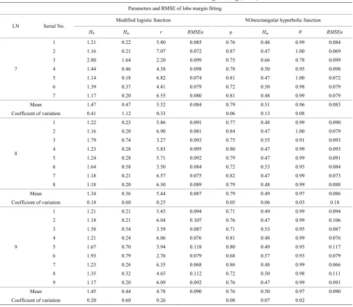
The liand hi represent the length of the vector projected from the point to leaf apexes on the leaf vein and the distance of the point on the lobe margin from the leaf vein respectively. The lobe margin model was established by fitting half of the lobe margin based on the normalized data: li = li/max(li), hi = hi/max(hi). The fitting effect for a leaf with 8 lobes was shown in Figure 4, and the parameters and validation were shown in Table 3.

Based on the RMSEn in Table 3, the fittings of the improved logistics model and the nonrectangular hyperbolic model are the same (both less than 10%). Thus, the models performed equally well.

Furthermore, the variation coefficients of the nonrectangular hyperbolic model parameters are lower than those of the improved logistic model parameters. It is indicated that the fitting of the nonrectangular hyperbolic model is better than that of the improved logistic model. The parameters of the nonrectangular hyperbolic model, including , Hm, and θ, i.e., the initial slope, final value and curvature, were estimated to be 0.79, 0.51 and 0.96 with 95% confidence intervals (CIs) of 0.74-0.83, 0.45-0.57 and 0.89-1.03 for Zibi5 with 7 lobes, 0.79, 0.49 and 0.97 with 95% CIs of 0.75-0.82, 0.46-0.52 and 0.95-1.00 for Zibi5 with 8 lobes, and 0.76, 0.50 and 0.97 with 95% CIs of 0.71-0.81, 0.47-0.53 and 0.95-0.99 for Zibi5 with 9 lobes respectively.

a. 14 angles for leaves with 7 lobes b. 16 angles for leaves with 8 lobes c. 18 angles for leaves with 9 lobes Note: The angles are bilaterally symmetric.

Figure 3 Angles between adjacent leaf veins and leaf valley lines

Table 3 Parameters and RMSE of lobe margin fitting (Zibi5)

Parameters and RMSE of lobe margin fitting

LN Serial No.

Modified logistic function NOnrectangular hyperbolic function

H0 Hm r RMSEn φ Hm θ RMSEn

7

1 1.21 0.22 5.80 0.085 0.76 0.48 0.99 0.084

2 1.16 0.21 7.07 0.072 0.87 0.47 1.00 0.069

3 2.80 1.64 2.20 0.099 0.75 0.66 0.78 0.099

4 1.44 0.46 4.38 0.098 0.78 0.50 0.95 0.098

5 1.14 0.18 6.82 0.074 0.81 0.47 1.00 0.072

6 1.39 0.37 4.41 0.079 0.72 0.50 0.98 0.079

7 1.17 0.20 6.55 0.080 0.81 0.48 0.99 0.079

Mean 1.47 0.47 5.32 0.084 0.79 0.51 0.96 0.083

Coefficient of variation 0.41 1.12 0.33 0.06 0.13 0.08

8

1 1.22 0.23 5.86 0.091 0.77 0.48 0.99 0.090

2 1.16 0.20 6.90 0.081 0.84 0.47 1.00 0.079

3 1.79 0.74 3.27 0.093 0.75 0.55 0.91 0.093

4 1.23 0.28 5.83 0.095 0.80 0.47 0.99 0.093

5 1.24 0.28 5.71 0.092 0.79 0.47 0.99 0.091

6 1.64 0.58 3.50 0.084 0.72 0.53 0.95 0.084

7 1.18 0.21 6.57 0.075 0.82 0.47 0.99 0.073

8 1.18 0.20 6.30 0.089 0.79 0.48 0.99 0.088

Mean 1.34 0.36 5.44 0.087 0.79 0.49 0.97 0.086

Coefficient of variation 0.18 0.60 0.25 0.05 0.06 0.03 0.18

9

1 1.21 0.21 5.45 0.094 0.71 0.49 0.99 0.094

2 1.18 0.21 6.04 0.107 0.76 0.47 0.99 0.106

3 1.58 0.54 3.59 0.087 0.71 0.53 0.95 0.087

4 1.21 0.24 6.06 0.076 0.81 0.48 0.99 0.076

5 1.67 0.70 3.94 0.118 0.80 0.49 0.95 0.117

6 1.93 0.79 2.76 0.079 0.68 0.57 0.93 0.079

7 1.23 0.26 6.35 0.068 0.86 0.48 0.99 0.066

8 1.35 0.32 4.65 0.112 0.72 0.50 0.98 0.111

9 1.17 0.20 6.09 0.092 0.76 0.47 0.99 0.091

Mean 1.45 0.44 4.78 0.090 0.76 0.50 0.97 0.090

Coefficient of variation 0.20 0.60 0.26 0.08 0.07 0.02

3.4 Leaf area calculation

As shown in Table 4, the formula for calculating the leaf area of different lobes was established. The area estimation based on main leaf vein length and shape parameters has a lower RMSEn and more stable coefficients than that based only on main leaf vein length. Thus, the formula of leaf area calculation based on main leaf vein length and shape parameters is better than that based only on main leaf vein length.

Table 4 Formula for leaf area calculation

LN Formula s RMSEn Formula RMSEn

7 S=1.02×s×(rL)2 _{1.758 0.06 S=0.86×L}2 _0.10 8 S=1.04×s×(rL)2 _{1.784 0.05 S=1.13×L}2 _0.11 9 S=1.07×s×(rL)2 _{1.804 0.05 S=1.14×L}2 _0.11 Note: s is the standard leaf area; S is the leaf actual area; L is the length of the longest leaf vein.

4 Application and significance

The castor bean leaf has a palm-like shape and a piecewise function, which may be a good option to depict the shape. An improved logistic model and a nonrectangular hyperbolic model were used to fit the leaf boundary, which showed great accuracy in fitting the lobe margin. Furthermore, the circular radius is almost

in the interval [0.75, 0.80] for the leaf apexes and the interval [0.35, 0.41] for the leaf valley points (Table 5). The radius slightly increased with the increase of lobe number for all sample groups, except the leaf apex of Yunbi2 and the leaf valley point of Xiangbi1. In summary, the results of this study may have theoretical significance for the visualization of castor bean leaves. Nondestructive and accurate methods of LA estimation are significant, especially under the field conditions[28]_{. In this study,} the empirical formula with leaf area, standard leaf shape, parameters of leaf radius and the number of lobes was established for LA calculation (where r is the radius of the standard leaf shape and L is the length of the leaf). Based on the general results, the LA of castor bean can be estimated more accurately from the leaf radius.

Table 5 Examples of diverse shapes and features of palmate leaves

Variety Radius of leaf apex Radius of leaf valley point 7lobes 8lobes 9lobes 7lobes 8lobes 9lobes Xiangbi1 0.805 0.783 0.753 0.373 0.385 0.370

5 Conclusions

To describe the leaf shape of castor bean, a standard simulation model of castor bean leaf shape was developed by using statistical and mathematical modeling methods. The model includes sub models, i.e., a circular model describing the landmark distribution, and functions used to depict lobe margins. The simulated standardized leaf is similar in morphology to areal castor bean leaf. This study would provide a new method for morphological simulation and leaf area of complex shape leaf with lobes. It would also have important reference significance for other crops digital research and phenotype model construction.

Acknowledgements

This research was supported by the National Forestry Science Data Platform of China (2005DKA32200-12), the State’s Key R & D Project of China (Grant No.2017YFD0301507), the Natural Science Foundation of Hunan Province, China (Grant No.2018JJ3227), and the Key R & D Project in Hunan Province, China (No.2017NK2382 and 2017NK2222). We would like to thank Chen Liyun and Zou Yingbin (Hunan Agricultural University, China) for their helpful discussions. We also thank Sun Ligang and GaoKailun (Hunan Agricultural University, China) and Ferdin and Corcuera (IRRI, Philippines) for their assistance in software design and data acquisition.

[References]

[1] Liebig H P. Modelling potential crop growth processes. Current Issues in Production Ecology, 1994; 2: 131–142.

[2] Thomson J A. On growth and form. Nature, 1917; 100: 21–22 [3] O’Shea B, Mordue-Luntz A J, Fryer R J, Pert C C, Bricknell I R.

Determination of the surface area of a fish. J. Fish Dis., 2006; 29(7): 437–440.

[4] Montgomery E G. Correlation studies in corn. Annual Report No. 24; Nebraska Agricultural Experimental Station: Lincoln, NB, USA, 1911; pp.108–159.

[5] Shi P J, Zheng X, Ratkowsky D A, Li Y, Wang P, Cheng L. A simple method for measuring the bilateral symmetry of leaves. Symmetry, 2018; 10(4): 118.

[6] Palaniswamy K M, Gomez K A. Length-width method for estimating leaf area of rice. Agron. J., 1974; 66(3): 430–433.

[7] Verwijst T, Wen D Z. Leaf allometry of Salix viminalis during the first growing season. Tree Physiol., 1996; 16(7): 655–660.

[8] Shi P J, Liu M D, Yu X J, Gielis J, Ratkowsky D A. Proportional relationship between leaf area and the product of leaf length width of four types of special leaf shapes. Forests, 2019; 10(2): 178.

[9] Shi P J, Liu M D, Ratkowsky D A, Gielis J, Su J L, Yu X J, et al. Leaf area–length allometry and its implications in leaf shape evolution. Trees,

2019; pp.1–13. Springer. https:doi.org/10.1007/s00468-019-01843-4. [10] Dornbusch T, Watt J, Baccar R, Fournier C, Andrieu B. A comparative

analysis of leaf shape of wheat, barley and maize using an empirical shape model. Ann. Bot., 2011; 107(5): 865–873.

[11] Gielis J. A generic geometric transformation that unifies a wide range of natural and abstract shapes. Am. J. Bot., 2003; 90(3): 333–338. [12] Shi P J, Xu Q, Sandhu H S, Gielis J, Ding Y L, Li H R, et al. Comparison

of dwarf bamboos (Indocalamus sp.) leaf parameters to determine relationship between spatial density of plants and total leaf area per plant. Ecol. Evol., 2015; 5(20): 4578–4589.

[13] Shi P J, Ratkowsky D A, Li Y, Zhang L F, Lin S Y, Gielis J. General leaf-area geometric formula exists for plants—Evidence from the simplified Gielis equation. Forests, 2018; 9(11): 714.

[14] Jani T C, Misra D K. Leaf area estimation by linear measurements in Ricinus communis. Nature, 1966; 212(5063): 741–742.

[15] Li X M, Wang X H, Wei H L, Zhu X G, Peng Y L, Li M, et al. A technique system for the measurement, reconstruction and character extraction of rice plant architecture. Plos One, 2017; 12(5): e0177205. [16] Zhang X. Studies on the measurement of plant leaf area based on image

processing. Harbin: Northeastern Agricultural University, 2009. (in Chinese)

[17] Rosin P L. Image difference threshold strategies and shadow detection. BMVC, 1995; 95: 347–356.

[18] Gonzalez R C , Woods R E , Eddins S L. Digital image processing using Matlab. Publishing House of Electronics Industry, 2009.

[19] Haralick, R M, Shapiro L G. Computer and robot vision, Volume I, Addison-Wesley, 1992; pp.28-48.

[20] Salazar-Colores S, Ramos-Arreguín J M, Echeverri C J O, et al. Image dehazing using morphological opening, dilation and Gaussian filtering. Signal, Image Video P., 2018; 12(7): 1329–1335.

[21] Annaldas B. Multi-parametric MRI study of brain insults (Traumatic brain injury and brain tumor) in animal models. Tempe: Arizona State University, 2014.

[22] Kruczyk M, Umer H M, Enroth S, Komorowski J. Peak finder metaserver - a novel application for finding peaks in ChIP-seq data. BMC Bioinformatics, 2013; 14(1): 280.

[23] Pierre S. Morphological image analysis: Principles and applications. Sensor Review, 1999; 28(5): 800–801.

[24] Li X M, Wang X H, Huang H, Li X P. A cereal crop canopy light distribution and photosynthesis model based on multiple factors - modeling and simulation. Pak. J. Bot., 2014; 46(3): 927–938.

[25] Ji L Q. A modified Logistic model for forecasting petroleum consumption in China. Journal of China University of Petroleum, 2011; 35(4): 177–181. (in Chinses)

[26] Rinaldi M, Losavio N, Flagella Z. Evaluation and application of the OILCROP–SUN model for sunflower in southern Italy. Agr. Syst., 2003; 78(1): 17–30.

[27] Seber G A F, Wild C J. Nonlinear regression. Hoboken. New Jersey: John Wiley & Sons, Inc., 2003; pp.62–63.