faunal remains, dated to 10,100 cal. BP, are well preserved and have highly resolved spatial
association with lithics and hearth features. Factors in the formation of the assemblage are
assessed through analyses of weathering, presence/absence of carnivore damage,
fragmenta-tion patterns, bone density, and economic utility. Taphonomic analyses indicate that human
transport and processing decisions were the major agents responsible for assemblage formation.
A spatial model of wapiti and bison carcass processing at this site is proposed detailing faunal
trajectories from the kill sites, introduction on site in a central staging area to peripheral marrow
extraction areas associated with hearths and lithic items. Data from mortality profiles, spatial
analysis, and economic analysis are used to interpret general economy and site function within
this period in Interior Alaska. These data and intersite comparisons demonstrate that considerable
economic variability existed during the Early Holocene, from broad spectrum foraging to efficient,
specialized terrestrial large mammal hunting.
Keywords:faunal analysis, Early Holocene, Alaska, spatial analysis, economic utility
Introduction
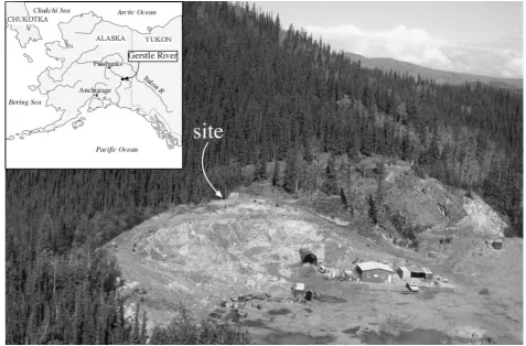
Information about economy and subsistence strate-gies are needed for an understanding of the post-glacial adaptations of high latitude foragers. This paper provides primary data on these subjects in the form of a multidimensional faunal analysis from an Early Holocene archaeological component at Gerstle River, located in the Tanana Basin in central Alaska. The Gerstle River site is located on a southern knob of a bedrock hill rising 137 m above the surrounding outwash plain one mile east of the large, braided Gerstle River (Fig. 1). Component 3 at the site is situated within stratified loess deposits (over 4 m thick), and consists of over 7000 lithic artefacts, dominated by microblade technology, burins, with unifacial and bifacial tools and by-products (Potter 2005). This material is directly associated with ten unlined hearth firepits and numerous faunal material
in a ‘living floor’ that forms a spatially integrated depositional set (see Potter 2005, 156–74). All cultural materials lay generally horizontally within a vertical span of ¡10 cm. No significant taphonomic dis-turbances such as cryoturbation were observed. Radiocarbon dated hearth samples (n 5 10) range from 8760¡40 BP (Beta-191558) to 9080¡50 BP (Beta-183108) and all are contemporary at 2 s (i.e. 95% confidence limits) when calibrated, averaging 8882¡17 BP, or 10164-9874 cal. BP (Potter 2005, 205-19). Sediment accumulation rates show rapid loess deposition during and after Component 3 was deposited (averaging 4 cm/100 years), helping to preserve the faunal remains.
The presence of numerous well preserved faunal remains in close association with cultural features and lithic artefacts is extraordinarily rare in Alaska, especially for the Late Pleistocene/Early Holocene. The following analysis is the first detailed published analysis of a well preserved archaeological faunal assemblage in eastern Beringia (Alaska and Yukon Territory) for this period, and therefore comparisons must be drawn from other areas such as Paleoindian Ben A. Potter, Department of Anthropology, University of Alaska
Fairbanks, 310 Eielson Building, Fairbanks, Alaska, 99775, USA; e-mail: [email protected]
and Late Prehistoric sites from Lower North America.
The faunal remains from Gerstle River can be treated as a single assemblage given the clear spatial association with lithic concentrations and hearth features that are contemporaneous (Potter 2005, 156-74). Given the high resolution in spatial pattern-ing within Component 3, there are a number of issues related to site structure, activity organization, and site function problems that can be addressed through faunal analyses. These problems are complicated and interrelated but can be presented within three general research questions regarding, (1) taphonomy, (2) models of faunal processing, and (3) models of general economy and site function. These problems are addressed through analysis of spatial patterning, weathering, carnivore damage, fragmentation, bone density, economic utility, and mortality profiles. A spatially integrated model of faunal processing and inferences about economy and site function are developed on these bases.
Methods
During excavation, all sediments associated with Component 3 were screened through 3?2 mm screens. All faunal fragments.3 cm in maximum dimension
were mapped in place. Faunal identifications were made through comparative collections of bison (Bison bison L.), wapiti (Cervus elaphus Erxleben), moose (Alces alces L.), and caribou (Rangifer tarandus L.) obtained from the University of Alaska Mammalogy Laboratory and the Department of Anthropology, and with the aid of various compara-tive guides (especially Brown and Gustafson 1979; Gilbert 1993; Hillson 1992; Schmidt 1972). Sorting, identification, sexing, ageing, and measurement methods generally follow Klein and Cruz-Uribe (1984) except where noted below. Each fragment was also examined for possible human, carnivore, or rodent modification such as cut marks, impact or puncture marks, or gnawing damage.
Each faunal specimen was examined for a number of coded variables, including taxonomic class, ele-ment portion (following Gifford and Crader 1977), side, degree of epiphyseal fusion, evidence of burning, weathering type (e.g., longitudinal cracking, erosion, root etching), completeness (complete, distal or proximal end and estimated per cent of diaphysis), faunal shape (long bone, flat bone, short/irregular bone, tooth/enamel), and weight.
Various terms are used in this analysis, and following calls for clarity and specificity (Casteel
time of recovery in the excavation. ‘MNE’ (minimum number of elements) refers to the minimum number of elements per element portion responsible for forming the faunal assemblage under investigation. Various means for estimating MNE based on long bone shafts have been discussed in the literature (Marean and Kim 1998; Mareanet al. 2001), however given the relative few identifiable long bone shafts without epiphyses, a fraction summation approach modified from Klein and Cruz-Uribe (1984) was used (note: no adjustment for size, sex, or age was made). ‘MNI’ (minimum number of individuals) represents the number of individuals necessary to account for the MNE within each species sample, taking into account element and side. ‘MAU’ (minimal animal unit) is defined as anatomical frequency counts, and is calculated (per taxon) as MNE/maximum number of element within one skeleton, and does not take into account size, sex, or age (see Binford 1984). Specific spatial and economic utility analytical methods are described below.
Results
Assemblage description and composition
Gerstle River Component 3 faunal remains consisted of 4,224 fragments and a total weight of 12?067 kg, with 192 identifiable specimens (71% of total by weight). Three taxa were identified, Cervus elaphus
(wapiti) (NISP 5 73), Bison sp. (NISP 5 33), and
Mammuthus sp. (mammoth) (NISP 5 1, worked ivory rod or point). The remaining 85 specimens were identified as large to very large mammals and/or Artiodactyla, representing bison, wapiti, or moose, and most likely representing bison or wapiti. Two bison specimens from Gerstle River (from disturbed contexts) were dated to about 9400 BP, and based on mtDNA analysis were interpreted to beBison priscus
Bojanus (steppe bison) (Shapiro et al. 2004); simila-rities in size with Component 3 specimens suggested that the latter were also Bison priscus. No medium sized mammals, avian, or fish remains of any kind were found within Component 3. While this could be the result of preservation conditions, the presence of trabecular bone in Component 3, a few small mammal bones found between Components 2 and 3, bear specimens found in Component 5, and avian
vertebra fragments (axial), and are probably bison or wapiti, but due to their highly fragmented nature, could not be distinguished from other large mammals such as moose. For analytical purposes, these specimens are lumped with the artiodactyl taxonomic category given the assemblage taxonomic composition and general size and morphology. Given the relatively high percentage of identified remains (71% by weight), it is suggested that most of the bones present within the excavated area were in fact identified, and form a suitable data set for further analysis.
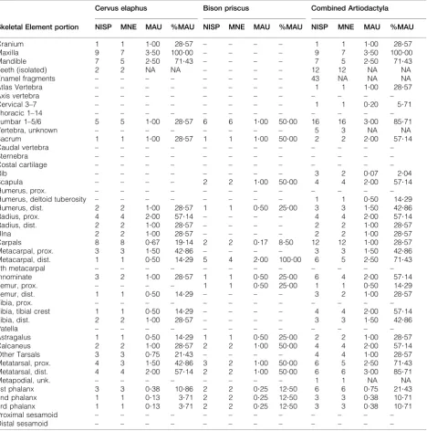
Table 1 lists NISP, MNE, and derivative MAU and %MAU values for the assemblage. It is important to note that MNE and MNI calculations are based on both long bone epiphyses and shaft fragments with diagnostic landmarks; however, it is possible that MNE based on these shafts will underestimate MNE relative to epiphyses, given that epiphyses are more readily identifiable to element portion and taxon (see Marean and Frey 1997). The most common elements besides maxillae are meta-carpals and metatarsals. MNI represented in Component 3 includes five wapiti and three bison, based on right maxillae/upper tooth rows (wapiti) and right distal metacarpals (bison). The unidentified artiodactyl element portions are generally different from those identified to species, with relatively high numbers of isolated teeth and enamel fragments, rib, scapula, and tibia fragments. When all artiodactyl specimens are analyzed, none of the MNE values indicate more than eight total large artiodactyls present within the component.
Taphonomy: weathering and carnivore damage
The bones, with the exception of compact bones like phalanges, carpals, and tarsals, are extremely fragile, and are generally falling apartin situ. Post-depositional
breakage was quite common, and was noted.
Weathering stages for each bone were not systematically recorded, as they are generally poorly preserved, ranging from Stages 4 to 5 (Behrensmeyer 1978). Weathering patterns in Component 3 fauna are consistent through-out the collection, with little difference relating to spatial position within the component, and consist of extensive root/acid etching leading to surface deterioration,
rootlet penetration, surface flaking, and some long-itudinal cracking of some of the larger long bone fragments. Due to this weathering, most of the cortical surfaces are deeply deteriorated or absent. Also, features such as cut marks are difficult to discern. Until more detailed microscopic examination is attempted, this possible data set cannot be further explored. Fig. 3 illustrates typical bone conditions andin situmaterial in faunal cluster F6a (see below).
The absence of well-defined cutmarks, though perhaps due to cortical bone deterioration, is not a necessary criterion for human butchery, as
Table 1 Faunal summary data per taxon
Skeletal Element portion
Cervus elaphus Bison priscus Combined Artiodactyla
NISP MNE MAU %MAU NISP MNE MAU %MAU NISP MNE MAU %MAU
Cranium 1 1 1?00 28?57 – – – – 1 1 1?00 28?57
Maxilla 9 7 3?50 100?00 – – – – 9 7 3?50 100?00
Mandible 7 5 2?50 71?43 – – – – 7 5 2?50 71?43
Teeth (isolated) 2 2 NA NA – – – – 12 12 NA NA
Enamel fragments – – – – – – – – 43 NA NA NA
Atlas Vertebra – – – – – – – – 1 1 1?00 28?57
Axis vertebra – – – – – – – – – – – –
Cervical 3–7 – – – – – – – – 1 1 0?20 5?71
Thoracic 1–14 – – – – – – – – – – – –
Lumbar 1–5/6 5 5 1?00 28?57 6 6 1?00 50?00 16 16 3?00 85?71
Vertebra, unknown – – – – – – – – 5 3 NA NA
Sacrum 1 1 1?00 28?57 1 1 1?00 50?00 2 2 2?00 57?14
Caudal vertebra – – – – – – – – – – – –
Sternebra – – – – – – – – – – – –
Costal cartilage – – – – – – – – – – – –
Rib – – – – – – – – 3 2 0?07 2?04
Scapula – – – – 2 2 1?00 50?00 4 4 2?00 57?14
Humerus, prox. – – – – – – – – – – – –
Humerus, deltoid tuberosity – – – – – – – – 1 1 0?50 14?29
Humerus, dist. 2 2 1?00 28?57 1 1 0?50 25?00 3 3 1?50 42?86
Radius, prox. 4 4 2?00 57?14 – – – – 4 4 2?00 57?14
Radius, dist. 2 2 1?00 28?57 – – – – 2 2 1?00 28?57
Ulna 2 2 1?00 28?57 – – – – 2 2 1?00 28?57
Carpals 8 8 0?67 19?14 2 2 0?17 8?50 12 12 1?00 28?57
Metacarpal, prox. 3 3 1?50 42?86 – – – – 3 3 1?50 42?86
Metacarpal, dist. 1 1 0?50 14?29 5 4 2?00 100?00 6 5 2?50 71?43
5th metacarpal – – – – – – – – – – – –
Innominate 3 2 1?00 28?57 1 1 0?50 25?00 6 4 2?00 57?14
Femur, prox. – – – – 1 1 0?50 25?00 1 1 0?50 14?29
Femur, dist. 1 1 0?50 14?29 – – – – 3 2 1?00 28?57
Tibia, prox. – – – – – – – – – – – –
Tibia, tibial crest 1 1 0?50 14?29 – – – – 4 4 2?00 57?14
Tibia, dist. 2 2 1?00 28?57 – – – – 3 3 1?50 42?86
Patella – – – – – – – – – – – –
Astragalus 1 1 0?50 14?29 1 1 0?50 25?00 2 2 1?00 28?57
Calcaneus 2 2 1?00 28?57 2 2 1?00 50?00 4 4 2?00 57?14
Other Tarsals 3 3 0?75 21?43 – – – – 4 4 1?00 28?57
Metatarsal, prox. 4 3 1?50 42?86 3 2 1?00 50?00 6 5 2?50 71?43
Metatarsal, dist. 4 4 2?00 57?14 2 2 1?00 50?00 6 6 3?00 85?71
Metapodial, unk. – – – – – – – – 1 1 NA NA
1st phalanx 3 3 0?38 10?86 2 2 0?25 12?50 6 6 0?75 21?43
2nd phalanx 1 1 0?13 3?71 2 2 0?25 12?50 3 3 0?38 10?71
3rd phalanx 1 1 0?13 3?71 2 2 0?25 12?50 3 3 0?38 10?71
Proximal sesamoid – – – – – – – – – – – –
Figure 2 Combined artiodactyl %MAU values illustrated on a wapiti skeleton (note rib and cervical portions are arbi-trary; skeleton adapted from Bubenik 1982)
it is quite possible to butcher an animal of any size without leaving a single mark on any bone. (Guildayet al. 1962, 64; see also Lyman 1987, 260–81)
However, extensive gnawing, pitting, or scoring was not observed on the Component 3 fauna, suggesting that carnivore or rodent modification was not a major factor in the formation of this assemblage. Morphological characteristics defined by Binford (1981) indicative of carnivore damage, including crenellated, scalloped, and jagged lateral edges, gnawed epiphyses, channeling, etc., were not observed on the specimens. Carnivore scavengers generally destroy spongy, greasy bones, such as vertebrae, innominates, and scapulae (Brain 1981; Blumenschine 1988; Marean and Spencer 1991; Marean and Frey 1997). The Gerstle River assem-blage do not show depressed MAU or %MAU values for these element portions, except for ribs (see Table 1). This pattern suggests that carnivore scavenging did not play an important role in element deletion or destruction at Gerstle River.
Taphonomy: fragmentation
All of the processes involved in breakage of faunal assemblages may not be known, but documentation of the fragmentation patterns is a necessary first step in evaluating taphonomic processes within a site (Todd and Rapson 1988). Because 30?7% by weight of the Gerstle River assemblage is made up of faunal remains unidentifiable to element, it becomes critical to assess fragmentation as it may relate to taphon-omy, butchery and processing practices, and other bone-altering agencies. For reasons stated above, small mammal, avian, and/or fetal material were probably not present in Component 3.
A number of variables were used to characterize fragmentation in the Gerstle River assemblage, including (1) ratios of number of fragments/NISP ratio, NISP/MNE, and NISP/MNI, (2) ratio of complete to incomplete element portions, (3) percen-tage difference in articular ends (proximal and distal), (4) amount of shaft remaining on humeri, and (5) percentage of shaft weight to all long bone weight.
In order to compare how bison and wapiti differ in fragmentation patterning and element representation, the number of fragments/NISP, NISP/MNE and NISP/MNI ratios for each taxon were compared. Number of fragments/NISP and NISP/MNE ratios are 4?9 and 1?1 for wapiti, 3?2 and 1?1 for bison, and 3?9 and 1?4 for combined artiodactyls respectively, suggesting that the fragmentation of identifiable specimens was relatively similar for wapiti and bison.
NISP/MNI ratios are 14?6 for wapiti, 11?0 for bison, and 23?9 for combined artiodactyls, indicating that bison remains are less well represented by the recovered identified specimens. Given the similarities in identifiable elements between wapiti and bison, it is suggested that bison remains were not more frag-mented and less identifiable. The hypotheses that more bison element portions were removed from the site or fewer were introduced cannot be refuted at this stage.
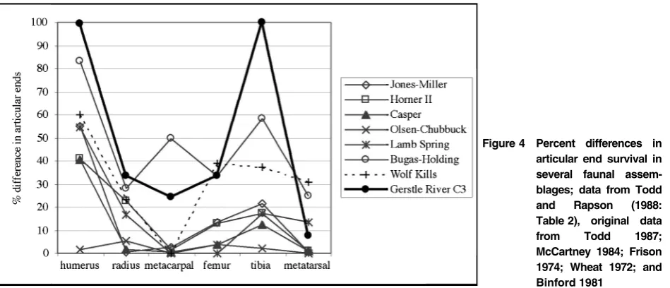
Only 28 specimens (excluding teeth) are complete or nearly complete (24% of all artiodactyl NISP), including carpals, tarsals, phalanges, and one meta-tarsal. Bison and wapiti had similar percentages of complete specimens across all elements. In addition, several vertebrae could also be considered complete, though only the centra and some articular processes are generally intact, the spinous, transverse, and many articular processes are generally broken, poorly preserved, or absent. This pattern is similar to that discovered by archaeologists in Paleoindian contexts (Todd and Rapson 1988; Frison 1974; Stanford 1984), though the Gerstle River assemblage should be considered more fragmented than those discussed in Todd and Rapson (1988), as there was only one long complete long bone element present. However, percentage difference in articular ends must be assessed in order to identify differential destruction or removal of certain element portions.
Generally more proximal element portions were removed or destroyed, whereas more distal element portions are better represented in the Gerstle River assemblage (Table 1). For all artiodactyls, most long bones exhibited this tendency within each element, only the radius showed an opposite trend. These data show that proximal element portions of appendicular long bones were differentially destroyed and/or removed from the Gerstle River assemblage.
latter site is interpreted to be a processing camp where long bones were fragmented for marrow extraction using cut-marks and impact point data (Todd and Rapson 1988). Todd and Rapson (1988, 314–9) further note that breakage of humeri near the thick-walled distal epiphysis could denote human-caused destruction rather than carnivore-caused destruction, which led to more of the shaft remaining with the distal epiphysis. This pattern is observed in the Gerstle River assemblage, where the distal humeri (n5 3) were fractured near the distal epiphysis.
Spatial analysis
Spatial aggregation for Component 3 is based on two hierarchical spatial groupings, provenience unit and
faunal cluster. Provenience unit is defined as the material associated with a specific three-dimensional location. Faunal clusters (F1-F9) are defined as faunal concentrations separated by areas devoid of faunal remains, and are based on 20 g/0?25 m2isopleths and distance between large bone fragments (Fig. 5). Given differences in bone modification and co-presence of lithic concentrations and features, cluster F6 was further subdivided into F6a and F6b (see below).
Two types of spatial analyses were conducted. The first uses spatial clustering of fauna to demarcate faunal clusters; these were analyzed using hierarchical clustering for heuristic purposes to assess differences among clusters. Hierarchical clustering was per-formed on all faunal clusters (except F8, see below) using Ward’s method (inner squared distance) and squared Euclidean distance measures, with raw values transformed to z-scores. The overall sample size (in terms of NISP) is relatively small, however, hierarchical clustering analysis is an exploratory
method, with few data limitations (essentially all relevant variables should be included and distance measures should be appropriate for the data). For the purposes of analysis, the faunal clusters are assumed to be complete and the excavated materials to be representative for each cluster (though portions of several faunal concentrations are truncated by the bluff edge). However, most faunal concentrations are spatially distinct and completely excavated, with density decreasing towards the excavation limits (with the sole exception of cluster F6a).
Clustering results are presented in Fig. 6 and are discussed below. The second analysis is based on overall spatial 3-point distributions across the site both within the context of the faunal clusters and of the entire component. Pertinent distributions are illustrated in Fig. 7. The faunal remains within Component 3 exhibit clear spatial patterning. Nine faunal clusters were visually identified based on the criteria listed above (see Fig. 5). Clusters F1, F3, F4, and F9 are directly associated with hearth areas and lithic concentrations. Clusters F2, F5, F7, F8, and to a lesser extent F6, are located in areas with little or no lithic concentrations and no cultural features. Interpreting the functional relationships among these faunal clusters and the features/lithics requires evalu-ation of various datasets. Table 2 lists summary faunal data within each faunal cluster, ordered by co-presence or absence of lithics and features. Cluster F8 is excluded given the small excavated area and relatively limited interpretive value.
Faunal clusters exhibited significant patterning based on association with lithic concentrations and features. For faunal clusters directly associated with lithic concentrations and features, average weight is relatively low, long bones are generally prominent
(54–72% of total weight), burn weights are relatively high (3–41%), skeletal unit type is dominated by limb bones. Interestingly, in areas where faunal remains co-occur with lithics and features, fragmentation levels are generally high, with nearly complete ele-ments and smaller fragele-ments interspersed. However, in areas where only faunal remains occur, the fragmentation values are generally low, suggesting
that these areas may have been used in such a way as to result in homogeneous fragmentation patterns. Both areas with high levels of articulation (Cluster F5 and F8) are in areas without lithics and features. Clusters F2 and F7 have no articulated specimens, whereas those clusters associated with lithics and features have moderate articulation levels (except F3 and F6b that have high and low articulation levels respectively). This patterning could indicate different processing activities in F1, F3, F4, and F9 vs. F2 and F7. The trimodal articulation %NISP wt. values (0, 12–17, 40–41) suggests that different processing modes occurred within spatially segregated portions of the site.
In areas devoid of lithic concentrations and features, %NISP wt. is considerably lower, though cluster F5 had by far the highest value. This pattern supports a demarcation between F5, which is characterized by articulated, non-fragmented, diag-nostic faunal remains and F2 and F7, which are characterized by unarticulated, fragmented, uniden-tified faunal remains. This pattern also suggests that faunal clusters found associated with lithics were typically more fragmented. %lower limb and %upper limb weight differences show similarities in clusters F3, F4, and F9 with a predominance of lower limb
Figure 5 Horizontal distribution of faunal remains
bones, where F2, F6b, and F5 show a predominance of upper limb bones. Clusters F1 and F7 show an even representation of upper and lower limb bones. In general, %lower limb weights were relatively higher in areas associated with lithic concentrations and features (51¡19 vs. 18¡21) and %upper limb weights were relatively higher in clusters devoid of lithics and features, suggestive of different processing in these areas.
Long bone ends generally seem to be spatially disassociated from shaft fragments, the latter found at the periphery of the faunal clusters. This pattern may result from breaking long bones for marrow and
tossing ends away from the processing area. Shaft weight (as a percentage of all long bones) varies among faunal clusters (26–82%). Three groups are apparent: one with values between 23–34% (F1, F3, F4, F9, F5), one with values of 58–63% (F2, F7), and one with values of 82% (F6). Faunal clusters F2 and F7 are interpreted as disposal areas based on a variety of data sets (see above), and the relatively high shaft weight percentages supports the greater fragmentation of long bones within these areas. The faunal clusters associated with hearths and lithic concentrations have generally low shaft weight percentages, suggesting activities resulting in lesser
degrees of fragmentation, like cracking long bones for marrow extraction.
While only a relatively small per cent of the total faunal remains in Component 3 were burned (14% by weight), almost all burned bones (black, brown charred are more common than calcined) are clustered directly in association with hearth features. Nearly half of the hearths do not contain burned bone, and wood charcoal was abundant in each hearth, suggesting that the bones were not system-atically used as fuel.
Wapiti and bison show considerable spatial inter-mixture. Skeletal unit types exhibited clustered distributions, with teeth fragments found at some distance from other skeletal unit types, generally in areas between hearths. Axial portions are mostly limited to cluster F5 and the immediate vicinity. Cluster F5 stands apart from the other groups in its relative lack of fragmentation and high levels of articulation. Interestingly, two of the three other clusters not associated with lithics have no articula-tions (F2 and F7), suggesting that these may represent bone dumps or discard areas.
The results of this spatial analysis show that considerable spatial patterning is evident within Gerstle River. In order to assess overall variability between the faunal clusters, hierarchical clustering was conducted, using co-occurrence with lithic concentrations, average weight, weight density, %shaft weight, %faunal shape, %burned, %skeletal unit type, %articulated total weight variables (trans-formed to z-scores) (Fig. 6). Three groups were formed: (A) F1, F4, F6b, F7, F9, (B) F2, F3, F6a, and (C) F5. Within Group A, bone marrow extrac-tion from long bones is hypothesized for F1, F4, F6b, and F9, as all are directly associated with features and lithic concentrations, with high fragmentation, low average weights, low articulation, high %burned weights, and high frequencies of long bones. F7 may represent a disposal area given lack of fragmentation, lack of articulation, and lack of associated features or lithics. Within Group B, two of the three clusters are not associated with lithics or features (F2, F6a) and may represent discard or disposal areas. The inclu-sion of F3 within this group is likely due to the presence of teeth and articulated lumbar vertebrae,
Table 2 Faunal cluster data summary. Note: for variables from Area to %Burn wt., data include all faunal fragments except for 13 not identifiable to cluster (n 5 4209 fragments), for variables from %NISP wt. to Skeletal Unit Type, data include all NISP (n 5 192). Fragmentation summary is based on average weight per fragment for each cluster (above or below the mean for all groups)
Faunal Cluster
Associated with features and lithics Not associated with features and lithics
F1 F3 F4 F9 F6b F2 F7 F5 F6a
Area (m2) 8?0 8?0 10?0 11?3 8?0 16?0 7?5 12?0 10?0
N fragments 487 417 672 936 489 28 268 500 412
Total wt (g) 2200?8 640?2 1297?9 1763?6 550?1 373?4 900?2 2847?0 1204?0
Avg. wt. (g) 4?5 1?5 1?9 1?9 1?1 13?3 3?4 5?7 2?9
Wt. Density (g/m2) 275
?1 80?0 129?8 156?1 68?8 23?3 120?0 237?3 120?4
Shaft wt. (% of all long bones)
33 26 27 34 82 63 58 23 82
Bone type zlong zlong zlong zlong zlong 2long zlong 2long 2long
%Unid. wt. 7 12 14 8 15 6 13 3 9
%Long wt. 58 54 71 62 72 43 64 42 50
%Flat wt. 19 2 1 14 3 13 16 17 18
%Teeth wt. 11 27 5 0 0 15 5 3 20
%Irreg. wt. 5 4 10 16 10 23 2 35 3
%Burn wt. 3 41 4 11 5 0 0 4 0
%NISP wt. 67 81 67 73 56 55 55 91 44
NISP wapiti/bison 50 60 90 100 57 67 17 72 63
MNI bison 1 1 1 0 1 1 2 1 1
MNI wapiti 1 1 1 2 1 1 1 2 1
Skeletal Unit Type Long bones Axial, teeth Long bones Long bones Long bones Axial, teeth Long bones Mixed Axial, teeth
%Axial wt. 21 45 0 3 6 43 2 40 35
%Teeth wt. 15 22 7 0 0 28 9 3 40
%U. limb wt. 19 0 21 27 60 29 43 49 10
%L. limb wt. 45 33 71 71 34 0 46 8 14
Skeletal Unit Type 2 App. Axial App. App. App. Axial App. Mixed Axial
%Axial wt. 36 67 8 3 6 71 11 43 75
%Append. wt. 64 33 92 97 94 29 89 57 25
Articulated %NISP wt. 15 41 12 14 0 0 0 40 17
Fragmentation Low High High High High Low Low Low High
which elevates %axial and %teeth. The differences between F2 and F7 may relate to different ‘sources’ of processing areas for these dumps, as these differences are shared by adjacent ‘processing areas’ (F3 and F2, and F4 and F7). Cluster F5 is clearly the most divergent from all of the other clusters in many ways. Cluster F5 is characterized by high abundance of large, mostly articulated specimens (high average weight and weight density), low %shaft weight, high %irregular bones, high %NISP weight, and is the most mixed in terms of skeletal unit type. Further interpretations of these clusters are provided below after density-mediated attrition and economic utility are addressed.
Skeletal part frequency analysis: bone density and %survivorship
Relationships among the skeletal parts actually found at Gerstle River, those expected to be found assuming whole carcasses were brought to the site, and those expected given MNE and MNI calculation are important in understanding processing decisions made by site occupants. The absence or low frequencies of various skeletal elements from the assemblage (notably cervical and thoracic vertebrae, ribs, and upper limb bones) could result from a number of reasons, including differential removal from the site and density-mediated attrition, a common problem of equifinality. In order to identify the relative weight of density-mediated attrition (such as in situ deterioration) and processing decisions by humans, bone density and economic utility (see further) are assessed.
A number of archaeologists (Grayson 1989; Lyman 1985; 1992; Marean and Frey 1997; Marean and Cleghorn 2003) noted that reverse utility curves could result not just from differential bone transport,
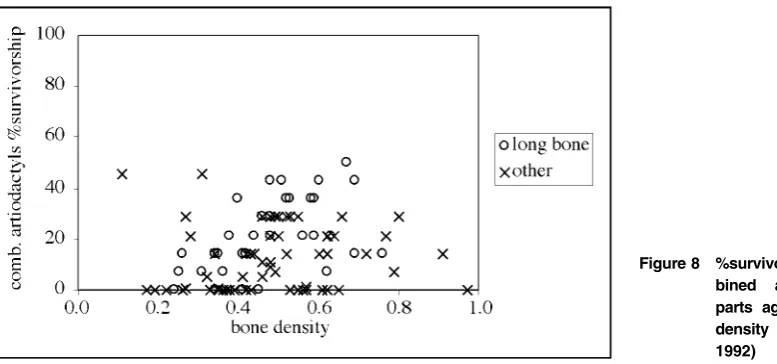
but from density-mediated destruction, which could be due to carnivore destruction,in situweathering, or other taphonomic agent. To evaluate the potential for density-mediated attrition, the %survivorship against bone mineral densities (g/cm3) for all available skeletal parts derived from Kreutzer (1992) was plotted. %survivorship is calculated by summing all of the present element portions for each bone density scan site and dividing by the expected numbers of surviving element portions for each scan site given 100% survivorship based on MNI per taxon (see Lyman 1994a, 239).
The results are illustrated as scatterplots (Fig. 8). The Spearman’s rho correlation coefficient of rank order (rs) between density and bison %survivorship is weakly positive and not significant (rs 5 0?11, p 5 0?292). Wapiti %survivorship has a slightly stronger (but still weak) positive relationship with density (rs5 0?32, p 5 0?001). Combined artiodactyl %survivor-ship has a weak positive relation%survivor-ship with density (rs 5 0?29, p 5 0?004). These results indicate that density-mediated attritional/taphonomic processes may not have been major factors in the formation of the Component 3 faunal assemblages. The weak positive correlation of wapiti %survivorship and bone density may be the result of disintegration of cancellous (or trabecular) bone through surface and
in situ weathering or the weight of overlying sediments. Bones with low mineral density, such as lumbar vertebrae, distal femora, and scapulae have %MAU values of 85?71, 28?57, and 57?14 respectively (comb. artiodactyls). The presence of low density bone portions suggests that the expected element portions based on MNI but not found at the site were not likely removed due to disintegration throughin situweathering or other density-mediated attrition.
Bone density measures were also used to test between density-mediated attrition and human-related differential transport or destruction of faunal elements. Grayson (1988, 70-1) suggested that assemblages exhibiting density-mediated attrition would show a significant positive correlation between %MAU and bone density, whereas assemblages exhibiting differential transport would show a sig-nificant positive correlation between %MAU and a utility measure (%MGUI or (S)FUI) and an insig-nificant correlation between %MAU and bone density (see also Lyman 1994a, 258–81). A third category can be posited, that of an assemblage from which elements were differentially transported to another location, showing a significant negative correlation between %MAU and %MGUI and an insignificant correlation between %MAU and bone
density. Following Rapson (1990) and Lyman
(1994a), the maximum density values for each MAU skeletal category were used to allow for correlation analysis, as defined in Lyman (1994a, Table 7.10).
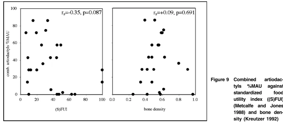
Using Metcalfe and Jones (1988) food utility index ((S)FUI) for caribou and Kreutzer’s (1992) bone density estimates for bison, Fig. 9 compares %MAU with bone density and (S)FUI. A negative correlation between %MAU and (S)FUI is apparent (rs5 20?35, p 5 0?087), whereas there is no correlation between %MAU and bone density (rs 5 0?09, p 5 0?691). Other food-related indices suggest a negative correla-tion between element abundance and food utility (see Table 3), especially with the relative lack of cervical vertebrae, thoracic vertebrae, ribs, femora, humeri, and proximal tibiae. This patterning places the Gerstle River assemblage within Lyman’s Class 2
(reverse utility, not winnowed or lagged/ravaged)
(Lyman 1994a, 258–63). Therefore, Gerstle
River assemblage is a good example where human differential transport or destruction of certain high yield elements (with respect to food utility) played a major taphonomic role in the formation of the faunal assemblage but density-mediated destruction did not. Specific food resources are considered next.
Skeletal part frequency analysis: utility indices
After considering the relative importance of various density-mediated attrition processes, we are in a better position to evaluate economic utilization of the carcasses brought to the site. The purpose of this analysis is to assess which food-related resources may have affected element abundance holding other resources constant. Desired food products may be related to specific skeletal elements (Binford 1978). Various models of economic utility have been proposed for ungulates; the ones considered here include caribou (Binford 1978; Metcalfe and Jones 1988) and bison (Emerson 1990; Brink and Dawe 1989; Brink 1997; 2001). No published economic utility models have been constructed for wapiti.
As Ringrose (1993, 151) and others have noted, the relationships between economic indices and element abundance are generally not precise enough to enable detailed statistical manipulation and hypoth-esis testing. Therefore, Spearman’s rho correlation coefficients are used in a heuristic, exploratory fashion, and alpha levels are set at 0?08 and 0?05. Following Brink (2001), patterns among positive and negative correlations among %MAU values and various utility indices are assessed for all elements and appendicular elements, as the latter are more
closely linked with specific resources, namely marrow and grease (Brink 2001; see also Ringrose 1993, 147–9).
Table 3 list the results of the correlations among utility indices and bison, wapiti, and combined artiodactyl %MAU. Significant correlations are presented as scatterplots in Fig. 10. In general, wapiti and combined artiodactyl %MAU, and to a lesser extent, bison %MAU are negatively related to meat and white grease related utility indices (such as total products, protein, total food, and food utility), and positively related to marrow indices for all elements
(n 5 26), though significance varies. These results are generally replicated for various caribou indices (Binford 1978; Metcalfe and Jones 1988), where (S)FUI, meat and modified general utility (MGUI) are negatively correlated with artiodactyl abundance. Overall, the patterning supports the argument that marrow was extracted from bison and wapiti carcasses or carcass portions, and that bone grease rendering was limited or not practiced at all. The most consistently demonstrated relationship between economic resource type and element abundance at the site is a reverse utility curve, with relatively high
(S)MAVGMAR (marrow) z0.08 z0.19 z0.10
(S)MAVGWG (white grease) 20.46* 20.34 20.41
(S)MAVGYG (yellow grease) z0.44 z0.62* z0.62*
(S)MAVGTF (total food) 20.19 20.26 20.16
(S)MAVGGRE (total grease) z0.14 z0.23 z0.11
(S)MAVGSKF (skeletal fat) z0.15 z0.21 z0.09
(S)AVGFUI (food utility) 20.21 20.26 20.13
Caribou (Metcalfe and Jones 1988)
(S)FUI (food utility) 20.35* 20.38* 20.20
Caribou (Binford 1978a)
Meat Index 20.19 20.30 20.12
Marrow Index z0.40** z0.51** z0.22
White Grease Index z0.08 z0.28 z0.07
MGUI 20.29 20.32 20.08
Bison bone density (Kreutzer 1992) z0.09 z0.09 20.11
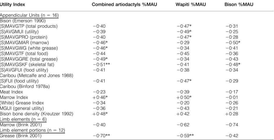
Table 4 Correlation (rs) of appendicular units (%MAU) with various utility indices. * significant at alpha 5 0.08 level
(2-tailed)**significant at alpha50.05 level (2-tailed)
Utility Index Combined artiodactyls %MAU Wapiti %MAU Bison %MAU
Appendicular Units (n516) Bison (Emerson 1990)
(S)MAVGTP (total products) 20.40 20.47* 20.31
(S)AVGMUI (utility) 20.39 20.49* 20.25
(S)MAVGPRO (protein) 20.40 20.47* 20.28
(S)MAVGMAR (marrow) 20.46* 20.29 20.50*
(S)MAVGWG (white grease) 20.46* 20.34 20.41
(S)MAVGTF (total food) 20.44 20.45 20.36
(S)MAVGGRE (total grease) 20.49* 20.34 20.43
(S)MAVGSKF (skeletal fat) 20.51** 20.41 20.48*
(S)AVGFUI (food utility) 20.41 20.38 20.34
Caribou (Metcalfe and Jones 1988)
(S)FUI (food utility) 20.41 20.47* 20.29
Caribou (Binford 1978a)
Meat Index 20.23 20.39 20.17
Marrow Index z0.46* z0.50* 20.01
(White) Grease Index 20.34 20.20 20.26
MGUI (general utility) 20.36 20.43 20.21
Bison bone density (Kreutzer 1992) z0.48* z0.42 z0.28
Limb elements (n56)
Marrow (Brink 2001) 20.40 20.62 20.74
Limb element portions (n512)
abundance of elements with high marrow yields and low abundance of elements with high meat and white grease yields. Furthermore, the fragments are not comminuted in a manner reflective of grease extrac-tion by boiling.
Given Marean and Frey’s (1997) critique of aggregating long bones with non-long bones in assessing utility indices, long bone were analyzed separately, and the results are listed in Table 4. Bison total products, utility, protein, marrow, white grease, total grease, and skeletal fat are all moderately negatively correlated with artiodactyl abundance.
Marrow Index is the only positive correlation. These results generally complement those obtained from examination of all elements; however the differences in marrow between Binford (1978) and Emerson (1990) suggests that further examination of their construction may be required.
The overall patterning in carcass economic utility suggests that for meat resources, the Gerstle River assemblage exhibits a reverse (bulk) utility strategy for bison, wapiti, and combined artiodactyls. For marrow resources, the available indices yield con-flicting correlations, and perhaps could be best
with high associated meat-values must have been brought to the site along with low-yield elements. While on-site, high-yield portions were likely pro-cessed for the meat, which was consumed and/or dried. If the Gerstle River represents a short-term camp, the high-yield anatomical portions could have been prepared for transport to a main residential camp. The elements associated with these high yield anatomical portions were not present at the site (fragmented or otherwise) after abandonment (e.g. ribs, thoracic vertebrae, and cervical vertebrae). While on-site, the occupants cracked elements with high marrow yields, e.g., tibiae, femora, humeri, radii, metacarpals, and metatarsals, while discarding elements with low marrow yields intact, e.g., tarsals, carpals, scapulae, and phalanges. No grease rendering or further processing of skeletal elements likely occurred at the site (see above).
Mortality profiles
Mortality profiles based on age are important for understanding general subsistence economies. Three techniques were used to estimate age of artiodactyls in Component 3: epiphyseal fusion of long bones, tooth eruption, and tooth wear. Given the limitations on epiphyseal fusion expressed above, and the generally fragmented nature of the Gerstle River
only. These data suggest that most if not all of the available wapiti long bones were from mature individuals, whereas the bison long bones represent mature and immature individuals (see Potter 2005, 307–8).
A total of 63 artiodactyl teeth were recovered from Component 3, including two left mandibles, three right mandibles, two left maxillae, five right maxillae, and an additional ten isolated teeth (Table 5). All tooth rows were identified as cervids on the basis of their morphology. Deciduous and permanent man-dibular tooth eruption in Cervus elaphus have been documented by Lowe (1967), Hillson (1986), and Jensen (1999). Based on morphological comparison of tooth wear, Gerstle River mandibular specimens fall within the 3?5-year-old class and 4?5–8?5-year-old classes (the oldest age classes in Jensen 1999). Using Klein and Cruz-Uribe’s (1984, 44–57) formulae for wapiti (red deer) crown height and age estimation age at death was estimated for 17 mandibular and maxillary M1 and M2 from nine tooth rows. The results indicate that three age groupings are present, all adults: 1?8–3?7 years (n 5 6 tooth rows and one isolated tooth), 5?2–6?3 years (n5 3 tooth rows and one isolated tooth), and 8?2 years (n51 tooth row). Minimum numbers of individuals for each age class given sided maxillae and mandibles are three for
Table 5 Crown height and age estimation.*minima due to tooth deterioration
Provenience Units Tooth L. (mm) Crown height (mm)
Age at death (months) using AGEpel5192
Age at death (months) using AGEpel5168, 210, and 215
Age estimation (years)
Tooth Rows
UA2000-54-12 L maxilla M1 26?1 14?6* 45 40 2?5
M2 29?1* 21?9 28 30
UA2000-54-774 R mandible M1 21?9 21?6 13 12 2?1
M2 30?1 29?6 20 20
M3 37?2 31?8 30 30
UA2001-71-646 R maxilla M2 – 13?1 69 75 6?3
UA2001-71-647 L maxilla M2 28?3 14?2 62 67 5?6
UA2003-54-50 L mandible M1 22?7* 6?7 111 98 8?2
UA99-62-45z49 R maxilla M1 28?5 18?4 25 22 3?7
M2 30?1 18?4 41 44
UA99-62-312 R maxilla M2 28?7 15?0 58 62 5?2
UA99-62-455 L maxilla M2 29?8 24?9 22 23 1?9
UA99-62-614 R mandible M1 24?4 8?5 93 82 3?4
M2 30?2 19?0 38 41
UA99-62-311 R mandible M3 39?8 25?5 35 36 3?0
Isolated teeth
UA2001-71-604 L maxilla M3 28?6 15?8 69 74 6?2
1.8–3.7 year class, two for 5.2–6.3-year class, and one for 8.2-year class. This may suggest that total wapiti MNI for Component 3 is six rather than five, though the greater variability in tooth wear in older animals may diminish the separation between the latter two age classes. The wear exhibited in the Gerstle River specimens was generally intermediate between the 3?5 year-old class and 4?5–8?5 year-old class (Jensen 1999), suggesting a close agreement between crown height formulae and tooth eruption/wear stages.
Given its small sample size, only tentative mortal-ity profiles and subsequent interpretations can be constructed with the Gerstle River faunal assem-blage. Nevertheless, these may have heuristic value given the dearth of published mortality profiles for any assemblage dating to the Late Pleistocene or Early Holocene in Alaska. In both catastrophic and attritional models, juveniles are expected to be abundant (Klein 1982; Stiner 1990). The Gerstle River wapiti mortality profile is consistent with a prime-dominated mortality profile (Stiner 1990; 1994), which may reflect selective ambush hunting of prey. Enloe (1993) suggested that efficient weap-onry able to kill at a long range could be inferred from prime-dominated mortality profiles. Stiner (1994, 307) notes that this type of pattern may also reflect ‘planned use of space’, and co-operative labour. At the very least, the age structure strongly argues for efficient human hunting practices, and offers further evidence against a carnivore-derived faunal assemblage. This pattern appears to be supported by prime wapiti and sheep represented at Dry Creek Components 1 and 2 (Guthrie 1983, 218, 220, 243, 252). While the sample size is small, the pattern does seem to suggest hunting preferences for prime adult ungulates during this period.
Discussion
TaphonomyFrom these analyses, is clear that the faunal assemblage did not form by means of carnivore accumulation. Patterns in weathering, fragmentation, and articulation indicate that carnivore modification and post-depositional taphonomic destruction was not a major factor in the formation of this assemblage. Various datasets indicate that no large-scale natural taphonomic agent disturbed the spatial patterning at Gerstle River. The spatial integrity of the faunal remains is thus highly resolved. With this high resolution and control on density-mediated attrition, inferences can be made about human processing patterns at the site and hunting strategies of the population that occupied this site.
Faunal processing model
In order to reduce and modify a carcass into anatomical units for transport, consumption, storage, and/or further processing (drying, etc.), various processing steps are needed. Lyman (1987; 1994a, 294–314) details various general processing activities and constraints on these activities. In the analyses below, the process of carcass reduction is modeled using Lyman’s framework, through the use of a spatial processing model and the inferred trajectories of anatomical units through a chain of processing events. Based on the spatial and economic analyses described above, the following model is proposed to explain the patterning observed in the Gerstle River faunal assemblage (see Fig. 11). The model incorpo-rates three stages of butchering activities, (1) carcass portions brought to the site and placed in a central ‘staging’ area, (2) element groups removed from carcass, taken to ancillary processing areas, where marrow was extracted, and (3) some specimens were discarded within areas that functioned as disposal areas, which were spaced at some distance from the areas of occupancy (denoted by hearth features and lithic items).
Three types of faunal clusters were identified in the course of this analysis: (1) staging area, (2) processing areas, and (3) dumps or refuse areas. One staging area (F5) was defined on the basis of articulated low-yield elements, relatively little fragmentation, and relative absence of long bones. Five processing areas (F1, F3, F4, F6b and F9) were defined on the basis of association with lithics and hearth features, low average weights (per fragment), high percentages of long bone ends and associated shafts, dominance of long bones, high percentages of burned bones, and generally higher levels of fragmentation. Additionally, the clusters are centered on hearths that have extensive amounts of burned and calcined bone directly within their matrix. Two dumps or refuse areas (F2 and F7) were defined on the basis of lack of association with lithics and features, high degree of fragmentation, and high percentages of long bone shafts, and lack of burned bone. The classification of F6a as an activity area is discussed later in the text.
Figure
11
Faunal
proce
ssin
g
groups (largely limbs) were removed from cluster F5 and transported to at least three and perhaps five areas (clusters F3, F4, F6b, and perhaps F1 and F9), where various types of processing took place. Four large cobbles were located at the periphery of cluster F5, and these may have been used as anvils to butcher the carcass segments (see Fig. 11). Clusters F1, F4, F6b, F9 (and to a lesser extent, F3) reflect very similar types of processing activities, where marrow was extracted from long bones. Lithic spatial patterning supports this model, as large, expedient boulder spall scrapers useful for processing game are different in their location at the periphery of lithic activity areas; whereas all other more formal lithic tool types (microblades, burins, unifaces, etc.) were found closely clustered near the hearths (Potter 2005, 747–81).
Cluster F3 had a somewhat different pattern from that of most clusters, with a preponderance of axial skeletal elements and teeth (by weight). This suggests that a different type of processing occurred there, although long bones were still present (including two bison metapodials). Faunal debris from cluster F3 was discarded in a ‘toss zone’ to the west and downslope (cluster F2), and faunal debris from cluster F4 were discarded to the east (cluster F7). These disposal areas were located on the periphery of the site occupation based on the feature and artefact distribution. Both disposal areas had no burned bones and similar high percentages of long bone shafts and relative lack of articular ends.
Two clusters remain somewhat ambiguous, F6a and F6b. While F6b shares many faunal characteristics with the other processing areas (F1, F3, F4, F9), there is no clear spatial ‘break’ with F6a to the south. F6a is interpreted to be: a continuation of the central staging area (F5) based on similar high average weights, high percentages of upper long bones, near absence of burned bones, and dominance of axial and teeth units, or, a specialized processing area based on more fragmented remains, more unidentified bone frag-ments. F6a may be an extension of the F5 staging area, but it showed evidence of some processing activities as well, including perhaps brain removal (F6a has the only large cranial fragments at the site) and extraction of meat and marrow from upper limb bones located south of Hearth 12. Cluster F6b is different from the other processing areas in that it has the highest percentage of long bone shafts (and lowest percentage of long bone ends), which could indicate more intensive processing of long bones or a meat-processing strategy which resulted in fragmented long bone shafts.
No articulated elements were observed in zones interpreted as disposal areas (F2 and F7), but, as might be expected, they were quite common in the staging area (F5) (Table 2). Areas F1, F4, and F9, interpreted as processing areas, have similar frequencies of articulated element, but F3 has higher values (largely due to the articulated vertebrae column within Feature 1). F6b has no articulated specimens, further suggest-ing that a different mode of processsuggest-ing occurred within cluster F6b. The similarity in articulation frequencies between processing areas F1, F4, F9, and F6a suggest a similar functional relationship between processing activities and bone articulation in these areas. Very few elements were refitted in these clusters, and most of the refits were located very close to each other within the same cluster.
These data suggest that Hearths 1, 3, 5, 10, 12, and 14 were associated with similar faunal processing tasks, namely extracting marrow from limb elements (primarily lower limb), as the faunal remains were centered directly on these features. These features have the highest burned bone percentages among all hearths (5–63% by weight), whereas the remaining hearths have no directly associated burned bone. Hearths 9, 13, 16 (and 18) were located on the periphery of these faunal clusters and the lack of burned bone directly associated with their matrices gives further evidence of distinct tasks with the other features with respect to faunal processing.
The similarities in the bison and wapiti assem-blages at Gerstle River in terms of NISP/MNI ratios, %MAU values, and fragmentation outweigh the differences, and the general pattern of processing outlined above likely applies to both bison and wapiti carcass portions brought to the site. From the skeletal element frequency analysis, almost all portions of the animals were likely introduced into the site with the exception of bison crania and mandibles. The food resources associated with ungulate cervical and thoracic vertebrae and ribs (high meat-yielding elements, corresponding roughly to the brisket and ribs) may have been (1) further processed (dried, smoked, etc.), (2) consumed at the kill site and not transported to the Gerstle River site, or (3) were introduced into the site and subsequently transported off-site or stored in an off-site location. The remain-ing portions after primary butcherremain-ing were intro-duced into the site for further processing. From this stage, the faunal trajectories of each anatomical portion diverged.
marrow extraction appears to be the result of mass processing event(s) rather than consumption and marrow extraction within the context of sequential events (see Potter 2005, 329–31). Marrow extraction and discard appear to be the final processes affecting the distribution and fragmentation of the faunal remains; bone grease rendering or boiling did not appear to be a major taphonomic agent.
Models of economy and site function: number of faunal processing events
The patterning of faunal elements with respect to taxonomic abundance and diversity, skeletal element abundance, burning, size, fragmentation, articula-tion, and spatial distribution within Gerstle River can be used to address issues of economic strategies, mobility, and site function. Number and duration of kill/transport/processing events and intersite compar-isons are examined here.
The number of faunal processing events reflected in the faunal assemblage is difficult to estimate. Each faunal cluster had an MNI of 2, and F5 and F7 had an MNI of 3. The similarities in MNI values for each cluster (between 25–38% of total component MNI) suggests that around three kill/transport events took place in this component. These scenarios are sup-ported by the evidence for contemporaneity described in Potter (2005, 156–74, 205–19, 620–69). As each main lithic subarea appears to be internally coherent and relatively undisturbed (i.e., contemporaneous), the faunal clusters associated with these areas may also be considered contemporaneous. Evidence for one kill or transport event includes the relatively limited spatial distribution of maxillae. The clear discrimination of lithic and faunal clusters and their relative lack of spatial distortion suggest that several processing events did not occur, nor is there a midden-like accumulation of material.
The faunal remains selectively culled from the site include element portions associated with high meat yields, including thoracic and cervical vertebrae, ribs, and to a lesser extent, upper limbs. This pattern reflects transportation of high utility portions. Given that almost no fragments of these elements were present in the assemblage, this indicates that either (a) there were limits to the number or amount of animal portions that could be removed due to small group
toolkits and curation (Potter 2005).
Models of economy and site function: intersite comparisons
Gerstle River faunal assemblage data can be com-pared with other faunal assemblages to examine broader issues of subsistence in the Late Pleistocene and Early Holocene in eastern Beringia such as taxonomic abundance and archaeological diet breadth. Large-bodied ungulates, especially wapiti and bison, have been key subsistence resources in the Paleolithic of the Old World and the New Worlds. Exploitation of red deer in Europe and Asia has been documented in detail from the Middle and Upper Paleolithic, where it dominates faunal assemblages (Pike-Tay 1991; Steele 2002). On the other hand, bison played a key role in early Paleoindian economies in the New World. While some have questioned early Paleoindian reliance on bison and other large mammals (Meltzer 1993; Grayson and Meltzer 2002; Cannon and Meltzer 2004), other studies have shown a clear pattern of specialized large mammal hunting during the Late Pleistocene and Early Holocene in North America (Waguespack and Surovell 2003; Haynes 2002; Hofman and Todd 2001; see also Kelly and Todd 1988; Frison 1998).
prime-juvenile female profile for bison. The relative absence of juvenile individuals suggests rather robust hunting strategies, in terms of efficiency and success. The lack of evidence of bone grease rendering and the completeness of a number of bones that could have been cracked for marrow extraction and consump-tion indicates that nutriconsump-tional stress was not present. The evidence for seasonality is meager and rather circumstantial. Based on macrofloral data from occupation surfaces (lingonberry berry and seeds, red raspberry seeds, that ripen in fall, and buds from
Alnus sp. or Salix sp., which form in the fall, are dormant in the winter), and wind direction based on void areas around hearths and modern wind patterns, a fall season of occupation is inferred. Male and female wapiti live apart for most of the annual cycle except for the autumn rut, and the presence of both at Component 3 (and the lack of calves) could be further evidence of a fall occupation. The Gerstle River Component 3 assemblage is more similar to Broken Mammoth Cultural Zone 3 (with 60% large mammal NISP), inferred to be a fall occupation, than with Broken Mammoth Cultural Zone 4 (with only 25% large mammal NISP) (Broken Mammoth data from Yesner 1996). This may indicate that consider-able seasonal variation in faunal exploitation exists during this period.
The Gerstle River data (in combination with data from Broken Mammoth and Swan Point (Holmes
et al. 1996; Yesner 1996) demonstrate that consider-able economic variability may exist at the level of Late Pleistocene/Early Holocene seasonal camps with respect to diet breadth. Gerstle River is situated within a time period where little is known about subsistence economies. Wapiti distribution and age in eastern Beringia (Alaska and Yukon Territory) has seen relatively little investigation (cf. Guthrie 1966). There are only seven published, dated assemblages with associated wapiti in Alaska. Gerstle River Component 3 is the latest evidence of wapiti exploitation in Alaska, though a few dated assem-blages are known from the Yukon Territory, notably at Pelly Farm (2920¡140 BP, GSC-127) (MacNeish 1964). The temporal and spatial distributions suggest that wapiti was present in Interior Alaska through much of the Holocene, and may have played a more important economic role than previously thought.
Acknowledgments
I wish to thank Anton Ervynck and two anonymous referees for providing insightful and useful comments regarding form and content of this article, and to
S. Craig Gerlach, Maribeth S. Murray, William B. Workman, and Joel D. Irish for comments on earlier versions of this research. I, of course, accept sole responsibility for any errors or omission. This work was funded in part by the Geist Fund, Bureau of Land Management (Robin Mills), and Northern Land Use Research, Inc. (Peter M. Bowers).
References
Behrensmeyer, A. K. 1978. Taphonomic and ecologic information from bone weathering.Paleobiology4, 150–62.
Binford, L. R. 1978. Nunamiut Ethnoarchaeology. New York: Academic Press.
Binford, L. R. 1981. Bones: Ancient Men and Modern Myths.New York: Academic Press.
Binford, L. R. 1984. Faunal Remains from Klasies River Mouth.
Orlando: Academic Press.
Blumenschine, R. J. 1988. An experimental model of the timing of hominid and carnivore influence on archaeological bone assem-blages.Journal of Archaeological Science15, 483–502.
Brain, C. K. 1981.The Hunters or the Hunted. Chicago: University of Chicago Press.
Brink, J. 1997. Fat content in leg bones ofBison bison, and applications to archaeology.Journal of Archaeological Science24, 259–74. Brink, J. 2001. Carcass utility indices and bison bones from the Wardell
kill and butchering sites, pp. 255–74 in Gerlach, S. C. and Murray, M. S. (eds.), People and Wildlife in Northern North America: Essays in Honor of R. Dale Guthrie (BAR International Series 944). Oxford: British Archaeological Reports.
Brink, J. and Dawe, B. 1989. Final Report of the 1985 and 1986 Field Seasons at Head-Smashed-in Buffalo Jump, Alberto
(Archaeological Survey of Alberta Manuscript Series 16). Edmonton: Archaeological Survey of Alberta.
Brown, C. L. and Gustafson, C. E. 1979.A Key to Postcranial Skeletal Remains of Cattle/Bison, Elk, and Horse (Washington State University, Laboratory of Anthropology, Report of Investi-gations 57). Pullman: Washington State University.
Bubenik, A. B. 1982. The endocrine regulation of the antler cycle, pp. 73–107 in Brown, R. D. (ed.),Antler Development in Cervidae. Kingville: Caesar Kleberg Wildlife Research Institute.
Cannon, M. D. and Meltzer, D. J. 2004. Early Paleoindian foraging: examining the faunal evidence for large mammal specialization and regional variability in prey choice. Quaternary Science Reviews23, 1955–87.
Casteel, R. W. and Grayson, D. K. 1977. Terminological problems in quantitative faunal analysis. World Archaeology 9 (2), 235– 42.
Emerson, A. M. 1990.Archaeological Implications of Variability in the Economic Anatomy of Bison bison. Unpublished Ph.D. disserta-tion, Department of Anthropology, Washington State University, Pullman.
Enloe, J. G. 1993. Subsistence organization in the Early Upper Paleolithic: reindeer hunters of the Abri du Flageolet, Couche V, pp. 101–14 in Knecht, H., Pike-Tay, A. and White, R. (eds.),
Before Lascaux: The Complex Record of the Early Upper Paleolithic. Boca Raton: CRC Press.
Frison, G. C. 1974. Archaeology of the Casper Site, pp. 1–111 in Frison, G. C. (ed.),The Casper Site: A Hell Gap Bison Kill on the High Plains. New York: Academic Press.
Frison, G. C. 1998. Paleoindian large mammal hunters on the Plains of North America.Proceedings of the National Academy of Science
95, 14576–83.
Gifford, D. P. and Crader, D. C. 1977. A computer coding system for archaeological faunal remains.American Antiquity42, 225–38. Gilbert, B. M. 1993. Mammalian Osteology. Columbia: Missouri
Archaeological Society.
Grayson, D. K. 1988. Danger Cave, Last Supper Cave, and Hanging Rock Shelter: the faunas.American Museum of Natural History Anthropological Papers66(1), 1–130.
Hoffecker, J. F. (eds.),Dry Creek: Archaeology and Paleoecology of a Late Pleistocene Alaskan Hunting Camp. Unpublished Report submitted to the National Park Service.
Haynes, G. 2002. The catastrophic extinction of North American mammoths and mastodons.World Archaeology33, 391–416. Hillson, S. 1986.Teeth.Cambridge: Cambridge University Press. Hillson, S. 1992.Mammal Bones and Teeth: An Introductory Guide to
Methods of Identification. London: Institute of Archaeology, University College.
Hofman, J. L. and Todd, L. C. 2001. Tyranny in the archaeological record of specialized hunters, pp. 200–15 in Gerlach, S. C. and Murray, M. S. (eds.), People and Wildlife in Northern North America: Essays in Honor of R. Dale Guthrie(BAR International Series 944). Oxford: British Archaeological Reports.
Holmes, C. E., VanderHoek, R. and Dilley, T. E. 1996. Swan Point, pp. 319–23 in West, F. H. (ed.), American Beginnings: The Prehistory and Paleoecology of Beringia.Chicago: University of Chicago Press.
Jensen, W. 1999. Aging elk.North Dakota Outdoors62(2), 16–20. Kelly, R. L. and Todd, L. C. 1988. Coming into the country: early
Paleoindian hunting and mobility.American Antiquity53, 231–44. Klein, R. G. 1982. Age (mortality) profiles as a means of distinguishing hunted species from scavenged ones in Stone Age archaeological Sites.Paleobiology8, 151–8.
Klein, R. G. and Cruz-Uribe, K. 1984.The Analysis of Animal Bones from Archeological Sites.Chicago: University of Chicago Press. Kreutzer, L. A. 1992. Bison and deer bone mineral densities:
comparisons and implications for the interpretation of archae-ological faunas.Journal of Archaeological Science19, 271–94. Lowe, V. P. W. 1967. Teeth as indicators of age with special reference
to red deer (Cervus elaphus) of known Age from Rhum.Journal of Zoology (London)152, 137–53.
Lyman, R. L. 1985. Bone frequencies: differential transport, in situ destruction, and the MGUI.Journal of Archaeological Science12, 221–36.
Lyman, R. L. 1987. Archaeofaunas and butchery studies: a taphonomic perspective, pp. 249–337 in Schiffer, M. B. (ed.), Advances in Archaeological Method and Theory, Vol. 10. New York: Academic Press.
Lyman, R. L. 1992. Anatomical considerations of Utility Curves in Zooarchaeology.Journal of Archaeological Science19, 7–22. Lyman, R. L. 1994a.Vertebrate Taphonomy.Cambridge: Cambridge
University Press.
Lyman, R. L. 1994b. Quantitative units and terminology in zooarch-aeology.American Antiquity59, 36–71.
MacNeish, R. S. 1964. Investigations in Southwest Yukon: archae-ological excavations, comparisons, and speculations.Papers of the Robert S. Peabody Foundation for Archaeology6(2), 199–488. Marean, C. W. and Cleghorn, N. 2003. Large mammal skeletal element
transport: applying foraging theory in a complex taphonomic system.Journal of Taphonomy1, 15–42.
Marean, C. W. and Frey, C. J. 1997. Animal bones from caves to cities: Reverse Utility Curves as methodological artifacts. American Antiquity62(4), 698–711.
Marean, C. W. and Kim, S. Y. 1998. Mousterian faunal remains from Kobeh Cave (Zagros Mountains, Iran): behavioral implications for Neanderthals and Early Modern Humans.Current Anthro-pology39, S79–S114.
Marean, C. W. and Spencer, L. M. 1991. Impact of carnivore ravaging on zooarchaeological measures of element abundance.American Antiquity56, 645–58.
Press.
Metcalfe, D. and Jones, K. T. 1988. A reconsideration of animal body-part utility indices.American Antiquity53(3), 486–504. Pike-Tay, A. 1991. Red Deer Hunting in the Upper Palaeolithic of
Southwest France: A Study in Seasonality (BAR International Series 569). Oxford: British Archaeological Reports.
Potter, B. A. 2005.Site Structure and Organization in Central Alaska: Archaeological Investigations at Gerstle River. Unpublished Ph.D. thesis, Department of Anthropology, University of Alaska Fairbanks, Fairbanks.
Rapson, D. J. 1990. Pattern and Process in Intra-Site Spatial Analysis: Site Structural and Faunal Research at the Bugas-Holding Site. Unpublished Ph.D. thesis, University of New Mexico, Albuquerque.
Ringrose, T. J. 1993. Bone counts and statistics: a critique.Journal of Archaeological Science20, 121–57.
Schmidt, E. 1972. Atlas of Animal Bones for Prehistorians, Archae-ologists and Quaternary Geologists. Amsterdam: Elsevier Publishing.
Shapiro, B., Drummond, A. J., Rambaut, A., Wilson, M. C., Matheus, P. E., Sher, A. V., Pybus, O. G., Gilbert, M. T. P., Barnes, I. Binladen, J., Willersley, E., Hansen, A. J., Baryshnikov, G. F., Burns, J. A., Davydov, S., Driver, J. C., Froese, D. G., Harington, C. R., Keddie, G., Kosintsev, P., Kunz, M. L., Martin, L. D., Stephenson, R. O., Storer, J., Tedford, R., Zimov, S. and Cooper, A. 2004. Rise and fall of the Beringian Steppe Bison.Science306, 1561–5.
Stanford, D. J. 1984. The Jones-Miller Site: a study of Hell Gap bison procurement and processing. National Geographic Research Reports16, 615–35.
Steele, T. E. 2002. Red Deer: Their Ecology and How They Were Hunted by Late Pleistocene Hominids in Western Europe. Unpublished Ph.D. thesis, Department of Anthropology, Stanford University.
Stiner, M. C. 1990. The use of mortality patterns in archaeological studies of Hominid predatory adaptations. Journal of Anthropological Archaeology 9, 305–51.
Stiner, M. C. 1994. Honor Among Thieves: A Zooarchaeological Study of Neanderthal Ecology. Princeton: Princeton University Press.
Todd, L. C. 1987. Analysis of kill-butchery bonebeds and interpreta-tion of Paleoindian Hunting, pp. 225–266 in Nitecki, M. H. and Nitecki, D. V. (eds.),The Evolution of Human Hunting. New York: Plenum Press.
Todd, L. C. and Rapson, D. J. 1988. Long bone fragmentation and interpretation of faunal assemblages: approaches to com-parative analysis. Journal of Archaeological Science 15, 307– 25.
Waguespack, N. M. and Surovell, T. A. 2003. Clovis hunting strategies, or how to make out on plentiful resources.American Antiquity68 (2), 333–52.
Wheat, J. B. 1972.The Olsen-Chubbuck Site: A Paleoindian Bison Kill
(Memoirs of the Society for American Archaeology 26). Washington, D.C.: Society for American Archaeology.