Evaluation of GOCE Satellite only Models along the River Nile

(1)

Evaluation of GOCE Satellite only Models along the

River Nile

Abdallah A. Saad, Mona S. El-Sayed*

Surveying Engineering Department, Faculty of Engineering- Shoubra, Benha University, Egypt

Abstract

Geoid is the equipotential surface of earth’s gravity field, which partially coincides with the mean sea level. The external Earth’s gravity field is represented by Global Gravitational Model (GGM) which is consisted of globally and homogeneously distributed terrestrial and satellite gravity observations. GOCE is one of the satellite missions that have been used to determine the gravity field of the earth. It mainly represents the long wavelength components of the gravity field which can be evaluated externally by using terrestrial data such as GPS levelling. 17 GOCE models are evaluated against EGM2008 and 134 GPS levelling stations. The RMSE of the undulation differences (N (GOCE models) – N (GPS levelling)) are considered the usual method for measuring the accuracy of the models. Another technique is used for evaluation, using the successive differences of the observed undulations against their corresponding values from the GOCE models. In this study, different types of GOCE models with different degree and order are examined against observed undulations and EGM2008 at three different distances. The first distance between the points is about 5 km which is the approximate distance between every two successive data points. The second distance is about 9 km which corresponds with the EGM2008 resolution, and the third case is about 85 km every two successive data points which is the average resolution of the assessed GOCE models. Numerical results showed that some of GOCE models gave comparable results with EGM2008 especially at level of undulation differences.

Keywords

GPS/Levelling, Geoid Undulation, GOCE Models, EGM2008, Rate of Change, Undulation Acceleration

1. Introduction

One of the principal scientific objectives of GOCE satellite mission was to recover the global gravity field with an expected accuracy of about 1–2 cm (in terms of geoid) or 1 mGal (in terms of gravity) at the level of a spectral resolution of about degree 200 in terms of spherical harmonics, which corresponds to about 100 km at the equator [1-3]. GOCE is the first satellite mission to measure gravitational gradients directly using a high-precision electrostatic gravity gradiometer by the differential acceleration technique [4], which was used to recover the medium-to-higher frequency signal of the gravitational field. The on-board GPS receiver provides the Satellite-to-Satellite Tracking (SST) data, which were used to determine the precise kinematic orbit with a cm-level accuracy [5], and consequently to recover the long-wavelength part of the gravity field.

Generally, there are several different numerical

* Corresponding author:

[email protected] (Mona S. El-Sayed) Published online at http://journal.sapub.org/ajgis

Copyright©2019The Author(s).PublishedbyScientific&AcademicPublishing This work is licensed under the Creative Commons Attribution International License (CC BY). http://creativecommons.org/licenses/by/4.0/

techniques applied to recover the global gravitational model (GGM) by processing the GOCE Satellite Gravity Gradient (SGG) observables. Probably the most commonly used techniques are: the direct approach (DIR), the time-wise approach (TIM), and the space-wise approach (SPW) corresponding to the three types of models which are determined by the GOCE High Level Processing Facility (HPF) [6-8].

In this study, the global geoid models produced by GOCE satellite mission are investigated: 17 GOCE models are assessed using 134 GPS levelling stations along the Nile River to evaluate the models’ performance in relation to each other on one hand, as well as, assessing their absolute agreement with terrestrial data and EGM2008 on the other hand.

The following are some descriptions for GOCE models; Models of the GOCE High-level Processing Facility (HPF) by ESA

• Direct (DIR) approach (maximum degree and order 300) - 5 data levels – Released data 01/11/2009 – 20/10/2013 - A priori data (EIGEN-5C (DIR1), ITG-Grace2010s (DIR2)) - Complementary data from LAGEOS + GRACE for lower degrees and orders

(2)

• Space-wise (SPW) approach (maximum degree and order 280) - 3 data levels – Released data 11/2009 – 31/7/2012 - GOCE-only models - A priori high-resolution models (e.g. EGM2008) used for variance and covariance modelling

Other GOCE-only models

• ITG-Goce02 (maximum degree and order 240) - Released data 01/11/2009 – 31/6/2010

• JYY_GOCE02S (maximum degree and order 230) - Released data 01/11/2009 – 31/08/2012

• JYY_GOCE04S (maximum degree and order 230) - Released data 01/11/2009 – 19/10/2013

Combined GOCE+GRACE models

• EIGEN-6S2 (maximum degree and order 260) - Released data GOCE 01/11/2009–24/5/2013, GRACE 2/2003–9/2012, LAGEOS 1985–2010

• GOCO01S, GOCO02S, GOCO03S and GOCO05S (maximum degree and order 280) - Released data GOCE 01/11/2009 –20/10/2013 (TIM5), GRACE 2/2003 –12/2013 (ITSG-Grace2014s)

• GOGRA02S and GOGRA04S (maximum degree and order 230) - Released data GOCE 01/11/2009 –19/10/2013, GRACE 8/2002–8/2009

The EGM2008 model is complete to spherical harmonic degree and order 2159, and contains additional coefficients extending to degree 2190 [9]. Also, it is supplied with a conversion model complete to degree and order 2160 for converting height anomalies to geoid undulations. It represents the highest resolution to date of 5 * 5 arc minute

(9km *9km) [10,11]. EGM2008 have been evaluated in different part of the world by several authors [12-14].

2. Data Used (Observed Undulations –

EGM2008 – 17 GOCE Models)

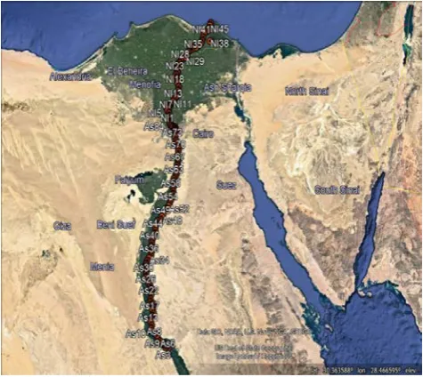
The study area extends from Assiut (Lat. 27° N) to Damietta (Lat. 31° N) along the Nile River. 134 fixed stations were established every about 5 km apart, covering total distance of 600 km, Figure 1.

Figure 1. The available points in the study area

Table 1. Characteristics of GOCE models and EGM2008

(3)

The geodetic coordinates, referenced to WGS84, of the 134 stations are obtained using GPS observations. Dual frequency GPS receivers are used. Those stations are tied to the nearest stations of the National Agricultural Cadastral Network (NACN) as reference stations. The orthometric heights of the fixed points are obtained by spirit levelling starting from the nearest bench marks of the ministry of irrigation. The mentioned available geodetic dataset, 134 GPS levelling stations have been observed by the Survey Research Institute (SRI) in several surveying sessions. Thus, the geoid undulations at the 134 fixed stations are obtained [15]. The geoid undulations of the 134 stations are extracted from EGM2008. Again, the geoid undulations of the 134 stations are extracted from the used 17 GOCE models, Table (1).

3. Investigating the Performance of the

Used 17 GOCE Models against the

GPS Levelling and EGM2008 over

the Test Area

The observed geoid undulations at the fixed stations are obtained from the well-known relation:

Ni = hi - Hi where N is the geoid undulation, h is the

ellipsoidal height obtained from GPS and H is the orthometric height obtained using spirit levelling. Using the latitude and the longitude of the observed stations, the corresponding geoid undulation values from EGM2008 and

the 17 GOCE models are obtained from the website http//icgem.gfz-postdam.de/ICGEM/ICGEM.html. So, the data that will be manipulated are the observed geoid undulations at the 134 stations and their corresponding values from EGM2008 and 17 used GOCE models.

3.1. Methodology and Results

Measuring the performance of the used 17 GOCE models over the test area will be examined at 3 levels of station spacing, 5, 9, 85 km. Station every five km to examine the models at the level of observed stations spacing. Nine km is to examine the models at the level of EGM2008 resolution. Eighty-five km is to examine the models at the level of the average resolution of the used GOCE models.

The observed undulation file is reduced once to 61 values and once more to 7 values out of 134 original values corresponding to about 9 and 85km respectively. The other files of EGM2008 and GOCE models are also reduced in the same way to be in correspondence with the reduced observation file.

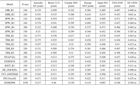
In most of the assessment works, a comparison between the model undulations against the observed undulations is the common way of assessment. This way produces a large mean and RMSE values of the resulting differences. Table 2 is extracted from [10] to show the usual way of comparison for the used GOCE models and EGM2008. The table contains RMSE of the differences between GPS levelling and the mentioned models for different data sets in different places;

Table 2. RMSE of the difference between GPS levelling and GOCE models, EGM2008 at different places

Model N max Australia 201 points

Brasil 1112 points

Canada 2691 points

Europe 1047 points

Japan 816 points

USA 6169 points

(4)

Therefore, it is much better to convert the undulations themselves into undulation differences. Considering the differences between every two successive undulations is suitable in the case that the data points are in longitudinal arrangement like the case of the data points in this research. Differences between an intermediate point and the other points could be considered when the data points cover an area. Differences between the undulations and their mean value (or the minimum value) could also be considered. Then the comparison (assessment) can be done using these differences. More details are in [15].

Undulation differences in this research are computed as: dNi = N(i+1) - Ni so, those differences are obtained from the

observed undulations, from EGM2008 undulations, and from the 17 GOCE models undulations. The assessments will be done once for the undulations themselves as usual and once more for the differences of every two successive values. Figure 2 illustrates the observed undulations and EGM2008 undulations, at the used 134 data points.

Figure 2. Observed undulation against EGM2008 undulations

3.1.1. EGM2008 Undulations against Observed Undulations in the Cases of 5, 9, 85 km Station Separations

The differences between the observed undulations and their EFM2008 corresponding values are computed and the statistics of those differences are obtained and illustrated in Table 3 and Figure 3.

Table 3. Statistics of the differences between observed and EGM2008 undulations, in cases of 5, 9, 85 km station separations

Station separation Min. m Max. m Mean m RMSE m 5 km 0.346 1.010 0.59 0.105 9 km 0.346 0.995 0.644 0.167 85 km 0.415 0.906 0.663 0.150

Figure 3. The mean and RMSE of the differences between observed and EGM2008 undulations in the three cases

In the three cases, EGM2008 has a mean shift about 65 cm from the observed undulations and about 16 cm RMSE. The results in the three cases are close to each other.

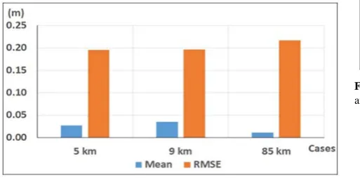
3.1.2. EGM2008 Differences against Observed Differences in Cases of 5, 9, 85 km Station Separations

Undulations successive differences are computed for both observed and EGM2008 undulations. The differences between the observed successive differences and their EGM2008 corresponding values are obtained and illustrated in Table 4 and Figure 4.

Table 4. Statistics of the diff. between EGM2008 differences and observed undulation differences, in cases of 5, 9, 85 km distances

Station

separation Min. m Max. m Mean m RMSE m 5 km -0.190 0.195 0.035 0.033 9 km -0.246 0.154 0.002 0.071 85 km -0.240 0.120 0.062 0.123

Figure 4. The mean and RMSE of the differences between observed and EGM2008 undulation differences in the three cases

The effect of using undulation differences instead of using the full undulation values in the comparison is very clear in reducing the mean and RMSE values. The results of the two cases of 5, 9 km station separation are close to each other because 5, 9 km distances are close to each other too. The case of 85 km is different mainly because its computations are dependent only on 7 data points.

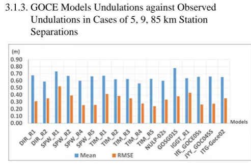
3.1.3. GOCE Models Undulations against Observed Undulations in Cases of 5, 9, 85 km Station Separations

(5)

Table 5. Statistics of the differences between observed undulations and GOCE models undulations (cm) in the three cases of 5, 9, 85 km distances

GOCE Models d/o

Difference between observed undulations and GOCE models (cm)

Mean (RMSE) 5km

GO_CONS_GCF_2_DIR_R1 240 67.7 (31.1) 66.4 (32.1) 70.8 (30.3) GO_CONS_GCF_2_DIR_R2 240 59.0 (35.3) 58.5 (36.2) 65.2 (33.2) GO_CONS_GCF_2_SPW_R1 210 73.2 (32.3) 74.8 (52.9) 80.9 (55.0) GO_CONS_GCF_2_SPW_R2 240 66.7 (39.4) 67.2 (39.6) 71.1 (42.1) GO_CONS_GCF_2_SPW_R4 280 60.1 (25.5) 58.8 (26.8) 63.0 (26.9) GO_CONS_GCF_2_SPW_R5 330 66.4 (25.7) 65.4 (26.3) 69.3 (28.7) GO_CONS_GCF_2_TIM_R1 224 67.2 (41.2) 68.1 (42.3) 74.2 (44.9) GO_CONS_GCF_2_TIM_R2 250 62.1 (38.4) 61.9 (38.3) 65.9 (39.0) GO_CONS_GCF_2_TIM_R3 250 62.3 (35.2) 61.1 (34.9) 66.4 (35.8) GO_CONS_GCF_2_TIM_R4 250 56.2 (27.9) 54.4 (28.3) 60.9 (29.7) GO_CONS_GCF_2_TIM_R5 280 62.8 (24.1) 61.1 (24.1) 65.2 (26.0) NULP-02s 250 60.0 (33.4) 58.9 (33.5) 64.5 (32.3) GOSG01S 220 78.0 (38.1) 76.7 ( 37.7) 77.7 (37.6) IGGT_R1 240 63.7 (43.1) 61.8 (43.7) 65.0 (38.6) IfE_GOCE05s 250 65.6 (26.3) 63.8 (26.6) 70.2 (22.2) JYY_GOC045S 230 65.9 (27.6) 65.1 (28.2) 68.5 (26.7) ITG-Goce02 240 65.3 (35.3) 64.4 (35.6) 69.7 (34.3)

Figure 6. The mean and RMSE of the differences between observed and GOCE models undulations, case of 9 km

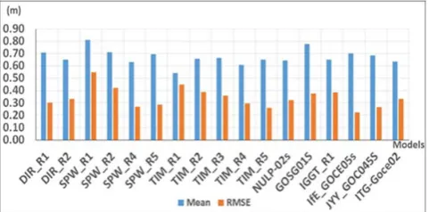
Figure 7. The mean and RMSE of the differences between observed and GOCE models undulations, case of 85 km

The differences between the undulations from the 17 GOCE models and the observed undulations are computed, Table 5 and Figures 5, 6, 7 illustrate the statistics of those differences;

From the above table and three figures, the behavior of the 17 GOCE models is almost the same towards the observed undulations in the three cases of the station separation. The best models, which have least RMSE, are SWP_R4 (280), SPW_R5 (330), TIM_R5 (280), IfE_GOCE05s (250), and JYY_GOCE04s (230). The worst model is SPW_R1 with d/o (210).

Figure 8. The mean and RMSE of the differences between observed and TIM_R5 GOCE model undulations, cases of 5, 9, and 85km

To follow the behavior of GOCE models in the three cases, the results of one of the best models, TIM_R5 (280), from 5, 9, 85km cases are illustrated in Figure (8).

The performance of TIM_R5 model is almost stable in the three cases of station separation.

3.1.4. Observed Undulation Differences against the

(6)

The differences between every two successive points in every GOCE model are computed. The differences between the observation differences and GOCE models’ differences

are obtained; the next table and three figures illustrate the statistics of these differences.

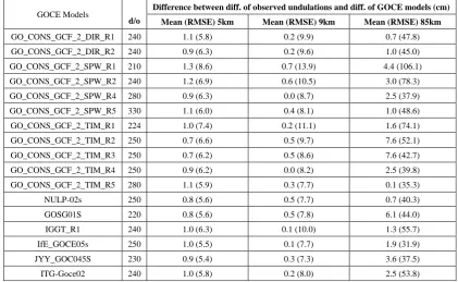
Table 6. Statistics of the differences of the undulation differences from the observations and GOCE models, (cm) in cases of 5, 9, 85 km distances

GOCE Models

d/o

Difference between diff. of observed undulations and diff. of GOCE models (cm)

Mean (RMSE) 5km Mean (RMSE) 9km Mean (RMSE) 85km

GO_CONS_GCF_2_DIR_R1 240 1.1 (5.8) 0.2 (9.9) 0.7 (47.8) GO_CONS_GCF_2_DIR_R2 240 0.9 (6.3) 0.2 (9.6) 1.0 (45.0) GO_CONS_GCF_2_SPW_R1 210 1.3 (8.6) 0.7 (13.9) 4.4 (106.1) GO_CONS_GCF_2_SPW_R2 240 1.2 (6.9) 0.6 (10.5) 3.0 (78.3) GO_CONS_GCF_2_SPW_R4 280 0.9 (6.3) 0.0 (8.7) 2.5 (37.9) GO_CONS_GCF_2_SPW_R5 330 1.1 (6.0) 0.4 (8.1) 1.0 (48.6) GO_CONS_GCF_2_TIM_R1 224 1.0 (7.4) 0.2 (11.1) 1.6 (74.1) GO_CONS_GCF_2_TIM_R2 250 0.7 (6.6) 0.5 (9.7) 7.6 (52.1) GO_CONS_GCF_2_TIM_R3 250 0.7 (6.2) 0.5 (8.6) 7.6 (42.7) GO_CONS_GCF_2_TIM_R4 250 0.9 (6.2) 0.0 (8.2) 2.5 (39.8) GO_CONS_GCF_2_TIM_R5 280 1.1 (5.9) 0.3 (7.7) 0.1 (35.3) NULP-02s 250 0.8 (5.6) 0.5 (7.7) 0.7 (40.3) GOSG01S 220 0.8 (5.6) 0.5 (7.8) 6.1 (44.0) IGGT_R1 240 1.0 (6.3) 0.1 (10.0) 1.3 (55.7) IfE_GOCE05s 250 1.0 (5.5) 0.1 (7.7) 1.9 (31.9) JYY_GOC045S 230 0.9 (5.4) 0.3 (7.3) 3.6 (37.5) ITG-Goce02 240 1.0 (5.8) 0.2 (8.0) 2.5 (53.8)

Figure 9. The mean and RMSE of the differences between observed and GOCE models undulation differences, case of 5 km

For all models, the mean values of the case of 9 km is less than their corresponding values in the case of 5 km while in the case of 85 they are larger than the two other cases. RMSE values in the case of 9 km are larger than the case of 5 km and the case of 85 km has very large values compared to the other two cases. Again, six differences only are not enough values to express the field in case of 85km. The last six models are from the best models. (TIM_R5) is still among the best models. The worst model is (SPW_R1) with d/o 210.

(7)

Figure 12. The mean and RMSE of the differences between observed and TIM_R5 GOCE model undulation differences, cases of 5, 9, and 85 km

The figure shows that the performance of (TIM_R5) is close in the first two cases but RMSE value in the case of 85km is too large compared to the first two cases.

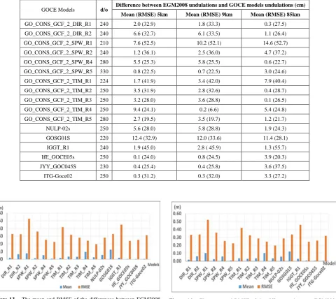
3.1.5. EGM2008 Undulations against GOCE Models Undulations in the Case of 5, 9, 85 km Station Separations

The differences between the undulation values from EGM2008 and from GOCE models are computed and their statistics are shown as follows;

Table 7. Statistics of the difference of EGM2008 and GOCE models undulations, (cm) in cases of 5, 9, 85 km distances

GOCE Models d/o Difference between EGM2008 undulations and GOCE models undulations (cm) Mean (RMSE) 5km Mean (RMSE) 9km Mean (RMSE) 85km

GO_CONS_GCF_2_DIR_R1 240 2.0 (32.9) 1.8 (33.3) 0.3 (27.5) GO_CONS_GCF_2_DIR_R2 240 6.6 (32.7) 6.1 (33.5) 1.1 (26.4) GO_CONS_GCF_2_SPW_R1 210 7.6 (52.5) 10.2 (52.1) 14.6 (52.7) GO_CONS_GCF_2_SPW_R2 240 1.2 (36.1) 2.5 (36.0) 4.7 (37.2) GO_CONS_GCF_2_SPW_R4 280 5.5 (25.3) 5.8 (25.5) 0.6 (22.7) GO_CONS_GCF_2_SPW_R5 330 0.8 (22.5) 0.7 (22.5) 3.0 (24.6) GO_CONS_GCF_2_TIM_R1 224 1.7 (41.9) 3.4 (42.0) 7.9 (40.4) GO_CONS_GCF_2_TIM_R2 250 3.5 (31.9) 2.8 (32.6) 0.4 (28.7) GO_CONS_GCF_2_TIM_R3 250 3.2 (28.0) 3.6 (28.8) 0.1 (26.5) GO_CONS_GCF_2_TIM_R4 250 9.4 (24.1) 0.2 (6.6) 5.4 (24.8) GO_CONS_GCF_2_TIM_R5 280 2.7 (19.5) 3.5 (19.7) 1.2 (21.7) NULP-02s 250 5.6 (28.0) 5.8 (28.8) 1.9 (24.3) GOSG01S 220 12.4 (32.9) 12.0 (33.6) 11.4 (28.1) IGGT_R1 240 1.9 (45.0) 2.8 ( 45.9) 1.3 (55.7) IfE_GOCE05s 250 0.1 (24.0) 0.8 (24.5) 3.9 (20.3) JYY_GOC045S 230 0.4 (25.4) 0.4 (25.8) 3.6 (37.5) ITG-Goce02 250 0.3 (31.2) 0.3 (32.0) 3.3 (27.2)

Figure 13. The mean and RMSE of the differences between EGM2008 and GOCE models undulations in the case of 5 km

(8)

Figure 15. The mean and RMSE of the differences between EGM2008 and GOCE models undulations, case of 85 km

The results in the case of 9 km are close to the results of the case of 5 km. The case of 85 km is better than the other two cases. SPW_R4 (280), If E_GOCE05S (250), JYY_GOCE04S (230), and TIM_R5 (280) are the best models, i.e. they are the nearest models to EGM2008. SPW_R1 (210), SPW_R2 (240), TIM_R1 (224), IGGT_R1 (240) gave the biggest RMSE among the other models.

Figure 16. The mean and RMSE of the differences between EGM2008 and TIM_R5 GOCE model undulations, cases of 5, 9, and 85km

The previous figure shows the mean and RMSE of the differences between EGM2008 and TIM_R5 GOCE model undulations in the three cases of 5, 9, and 85km.

The figure shows that the model TIM_R5 has nearly stable results in the three levels of station separation.

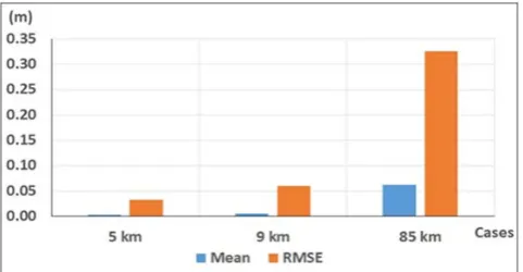
3.1.6. EGM2008 Undulation Differences against the Corresponding Values from GOCE Models in Cases of 5, 9, 85 km Station Separations

The differences between EGM2008 undulation differences and GOCE model’s undulation differences are computed; the following table and three figures illustrate the statistics of these differences.

Figure 17. The mean and RMSE of the differences between EGM2008 and GOCE models undulation differences, case of 5 km

Table 8. Statistics of the diff. between EGM2008 differences and every GOCE model differences (cm) in the three cases of 5, 9, 85 km distances

GOCE Models d/o Difference between the diff. of EGM2008 undulations and diff. of GOCE models (cm) Mean (RMSE) 5km Mean (RMSE) 9km Mean (RMSE) 85km

(9)

RMSE values in the case of 9 km are larger but not far from the case of 5 km. The case of 85 km has very large values compared to the other two cases. Recalling that only six differences are used in the case of 85km and they are not enough number of values to express the field. The models gave close results to each other’s except SPW_R1 (210), SPW_R2 (240), TIM_R1 (224), IGGT_R1 (240) gave bigger RMSE values among the other models. Still TIM_R5 is among the best models.

Figure 20. The mean and RMSE of the differences between EGM2008 and TIM_R5 GOCE model undulation differences, cases of 5, 9, and 85km

The figure shows the closeness of the first two cases and the large RMSE of the third case.

4. Conclusions

Using the undulation differences in the comparisons (evaluation) showed much better consistency than using the

comparisons of the undulation themselves. The differences and RMSE values of the first case are much smaller than their corresponding values of the second case. So, using undulation differences is much readable than using the full undulations. Then the adopted differences can be converted to full values using one trusted full undulation. The used GOCE models can be divided into subgroups; 2 DIR, 4 SPW, 5 TIM, and 6 others. The results inside every group are improved with the production year of the model. DIR model of 2011 is better than DIR model of 2010. The same for the two groups of 4 models of SPW and 5 models of TIM. The models of d/o 210, 220, and 224 are always among the worst models. The best models always include models of d/o 280 and 330.The results of the cases 5, 9 km station separation are close to each other’s with respect to most of the used models. Seven undulations, six differences, will be considered insufficient data in the case of 85 km.

TIM_R5 is always among the best models compared to the observed data and EGM2008. It will be taken as a representative to the used GOCE models. Overall the used 134 points, and in the comparison with EGM2008 undulations, this model has 2.7 and 19.5cm as mean and RMSE respectively. In the comparison with EGM2008 undulation differences, this model has 0.3 and 3.3cm as mean and RMSE respectively.

In comparing TIM_R5 undulations with the observed undulations, it gave 62.8 and 24.1cm for the mean and RMSE respectively. In comparing the undulation differences with the observed undulation differences, it gave 1.1 and 5.9cm as mean and RMSE respectively. To sum up, in the comparison of EGM2008 undulations with the observed undulations, the mean differences and RMSE were 65 and 16cm respectively. And in the case of comparing EGM2008 undulation differences with their corresponding observed values, the mean and RMSE were 0.8 and 4.7cm respectively. Recalling that TIM_R5, which is adopted here to represent GOCE models because it is one of the best models. It is a satellite only model with d/o 280 and it is produced in the year 2014 and it is produced from 4 yeas GOCE released data 01/11/2009 – 20/10/2013.

(10)

REFERENCES

[1] J., Agren, & R., Svensson “Postglacial Land Uplift Model and System Definition for the New Swedish Height System RH 2000. LMV-Rapport 2007: Reports in Geodesy and Geographical Information Systems. Gavle, Sweden. 124p. ISSN 280-5731, 2007.

[2] M., Bilker- Koivula “Development of the Finish height conversion surface FIN 2005N00”. Nordic Journal of Surveying and Real Estate Research. Vol. 7:1. pp. 76-88. ISSN 1459-5877, 2010.

[3] M., Bilker- Koivula “Assessment of high resolution global gravity field models for geoid modelling in Finland”. Proceeding of the international Symposium on Gravity, Geoid and Height Systems. IAG Symposium, Vol. 141, 2015. [4] S. L., Bruinsma, J. C., Marty, G., Ballmino, R., Biancale, C., Foerste, O., Abrikosov, & H., Neumayer “GOCE Gravity Field Recovery by Means of the Direct Numerical Method”. ESA Living Planet Symposium, 2010. Bergen, Norway. [5] S. L., Bruinsma, C., Foerste, O., Abrikosov, O., Marty, M. H.,

Rio, S., Mulet & S., Bonvalot “The new ESA satellite- only gravity field model via the direct approach”. Geophysical Research Letters. Vol. 40:14, pp. 3607-3612.

DOI: 10.1002/gr1.50716, 2013.

[6] Q., Chen, Y., Shen, H., Hsu, X., Zhang, W., Chen & L., Lou ”Tongji- GRACE01- A GRACE- only Static Gravity Field Model Recovered From GRACE Level-1B Observations using Modified Short Arc Approach”, 2013. [7] N.K. Pavlis, S.A. Holmes, S.C. Kenyon, and J. K. Factor

“The development and evaluation of the earth Gravitational Models 2008 (EGM 2008)”, Journal of Geophysics, Vol. 117, 1-38, http/doi.org/10.1029/2011jb008916, 2012.

[8] R., Pail, H., Goiginger, R., Mayrhofer, W., Schuh, J. M. Brockmann, I., Krasbutter, E., Hoeck, & T., Fecher ”GOCE gravity field model derived from orbit and gradiometry data applying the time-wise method”. ESA Living Planet Symposium, 2010. Bergen, Norway.

[9] T., Saari and M., Koivula “Evaluation of GOCE-based Global Models in Finnish Territory”. National Land Survey of Finland. URI: http//hdl.handle.net/10183/224774, 2015. [10] International Center for Global Gravity Field Models

(ICGEM), Available online

http://icgemgfz-potsdamde/ICGEM/2018.

[11] P. A., Odera “Assessment of EGM2008 using GPS/leveling and free-air gravity anomalies over Nairobi County and its environs”. South African Journal of Geomatics, Vol.5, No. 1, 2016, DOI http://dx.doi.org/10.4314/Sajg.v5i1.2.

[12] J., Huang, and M., Veronneau “Assessment of recent GRACE and GOCE release 5 global geopotential models in Canada. Newton’s Bull. 5: 127-148, 2015.

[13] A. P., Odera, Y., Fukuda “Towards an Improvement of the geoid model in Japan by GOCE data: a case study of the Shikoku area”. Earth Planets Space 65(4): 361-366 doi:10.5047/eps.2012.07.005, 2013.

[14] H.A., Abd-Elmotaal “Validation of GOCE models in Africa”. Newton’s Bull. 5:149-162, 2015.