Application of Method of Adjustable Model for
Identification of Linear Object with Uncertain
Parameters and Disturbance
Bukhar Kussainov
Institute of Control Systems and Information Technologies, Almaty University of Power Engineering and Telecommunications, Almaty, Republic of Kazakhstan
Abstract
In a wide variety of parametric uncertainties and external disturbance estimation and attenuation methods uncertainties and disturbance are lumped together and an observation algorithm is employed to estimate the total disturbance. While in certain cases of application can be required the separate estimation or identification of uncertain parameters itself and a disturbance. In the paper the separate and simultaneous identification (estimation) of unknown and/or changing parameters and an external disturbance of a linear object is considered. For this porpose the known procedure of synthesis of adaptive observer for estimation of parameters and state coordinates of a n-th order linear object is used taking into account the influence of the scalar external disturbance operating on this object. Developed adaptive observer provides asymptotic stability of processes of separate and simultaneous identification of uncertain parameters and an external disturbance of a n-th order linear object. Asymptotic stability of proposed observer is proved by Lyapunov’s direct method. As an example of using of the offered adaptive observer the structure and algorithm of joint identification of the moment of inertia (parameter) and the torque of resistance (external disturbance) of mechanical load of dc electric drive model are obtained. Asymptotic stability of processes of joint identification of the parameter and external disturbance of drive model is proved. Simulation results of identification processes and their using for control system adaptation are shown on graphs of transition processes. Designed algorithm for the joint identification of parameter and external disturbance of plant provide adaptive stabilization of desirable dynamic properties of control system with adaptive observer.Keywords
Uncertainties and disturbance, Estimation algorithm, Adaptive observer, Adaptive control system1. Introduction
Difficult dynamical controlled systems (aircrafts, mechatronic systems, technological processes, etc.) in the course of work are characterized by uncertain (unknown) and/or changing parameters (coefficients of the differential equations) and an external disturbance action. Parametric uncertainties and a disturbance can cause a deterioration of performance quality and lead even to an instability of control system. To keep the desired control quality of such plants it is necessary to reject an external disturbance and suppress uncertainties of parameters. The solving of this problem is carried out due to estimation (observation, identification) of uncertain parameters and an external disturbance and then using their estimates for the adaptation
* Corresponding author:
[email protected] (Bukhar Kussainov) Published online at http://journal.sapub.org/control
Copyright©2019The Author(s).PublishedbyScientific&AcademicPublishing This work is licensed under the Creative Commons Attribution International License (CC BY). http://creativecommons.org/licenses/by/4.0/
of control system to perturbations of parameters and a disturbance.
separate estimation of parameters we’ll use the method of generalized adjustable model [8,9] in which the closed contours of estimation of parameters of a n-th order linear object are self-adjustable (adaptive) by the identified parameters. Therefore, the adjustable model is called the adaptive observer in [9] and the adaptive observing device for identification of parameters in [10], besides, the procedure of creation of adaptive observer for a n-th order linear object and the proof of stability of its work are given in [9-12]. This adaptive observer allows also the estimation of unknown state coordinates of a n-th order linear object necessary for implementation of control laws.
In this paper the model of a n-th order linear object with unknown parameters is in addition considered with an unknown external disturbance. It is offered for the known adaptive observer to add the identification contour of external disturbance, it is proofed the stability of adaptive observer for separate and simultaneous identification of unknown parameters and disturbance as well as it is considered the application of offered adaptive observer for the first order linear object with an external disturbance.
This paper is structured as follows. In Sections 2 and 3 for the adaptive observer of identification of parameters and a disturbance of linear object the structure is developed and the stability is proved, respectively. In Sections 4 and 5 for a linear model of dc electric drive with a variable load the adaptive observer identifying a parameter and a disturbance is designed and its stability is proved, respectively. In Section 6 the simulation results of a control system with the adaptive observer estimating a parameter and a disturbance of dc electric drive are showed. Finally, in Section 7 the main conclusions of this paper are given.
2. The Structure of Adaptive Observer
for Identification of Parameters and
Disturbance of Linear Object
Let the linear control object (plant) has: 1) the known n-th order linear structure in which 𝑥 = 𝑥1, 𝑥2, … , 𝑥𝑛 Т is the
vector of state coordinates; 2) the known scalar input 𝑢 and output 𝑦 signals and 𝑦 = 1,0, … ,0 𝑥 = 𝑥1; 3) unknown
parameters; 4) an unknown scalar external disturbance 𝑓; 5) the unknown 𝑛 − 1 – dimensional vector of state coordinates 𝑥 ′= 𝑥2, 𝑥3, … , 𝑥𝑛 Т.
The considered plant we’ll describe by means of the following equation:
𝑦 =𝐵0𝑠𝑛 −1+𝐵1𝑠𝑛 −2+...+𝐵𝑛 −1
𝑠𝑛+𝐴1𝑠𝑛 −1+...+𝐴𝑛 𝑢 +
𝑅 𝑠
𝑠𝑛+𝐴1𝑠𝑛 −1+...+𝐴𝑛𝑓, (1)
where 𝑠𝑖 ≡ 𝑑𝑖 𝑑𝑡𝑖 , 𝑖 = 0, 𝑛 is the differentiation operator; 𝐴𝑖 𝑖 = 1, 𝑛 , 𝐵𝑖 , 𝑖 = 0, 𝑛 − 1 are the
unknown coefficients (parameters) of plant; 𝑅 𝑠 is the polynom depending from a place of action of an external disturbance f.
Let’s assume that
𝑅 𝑠 = 𝐵0𝑠𝑛−1+ 𝐵1𝑠𝑛−2+. . . +𝐵𝑛−1,
i.e. the unknown scalar external disturbance f also operates at the input of plant as the known scalar input signal u.
According to the technique stated in [10, 11] for identification of parameters 𝐴𝑖 , 𝐵𝑖 we’ll divide the
numerator and the denominator of transfer function (1) of plant by the 𝑛 − 1 –th degree polynom which roots are real negative single numbers:
𝑠 + 𝜆2 𝑠 + 𝜆3 … 𝑠 + 𝜆𝑛 ,
where 𝜆𝑖 > 0 𝑖 = 2, … , 𝑛 .
Having decomposed the numerator and the denominator to simple fractions let’s write the Eq. (1) in the following form:
𝑦 = 𝑏1+𝑏2
1
𝑠+𝜆2+⋯+𝑏𝑛𝑠+𝜆𝑛1
𝑠−𝑎1−𝑎2𝑠+𝜆21 −⋯−𝑎𝑛𝑠+𝜆𝑛1 𝑢 + 𝑓 , (2)
where 𝑏1= 𝐵0 ; 𝑎1= 𝜆2+ ⋯ + 𝜆𝑛 − 𝐴1 ; 𝑏𝑖 , 𝑎𝑖
𝑖 = 2, … , 𝑛 are incorporated with parameters 𝐴𝑖, 𝐵𝑖 and
𝜆𝑖 via more difficult relations.
Let’s write the Eq. (2) in the following form:
𝑦 𝑠 + 𝜆1− 𝜆1− 𝑎1− 𝑎2
1
𝑠 + 𝜆2− ⋯ − 𝑎𝑛
1 𝑠 + 𝜆𝑛 =
𝑏1+ 𝑏2 𝑠+𝜆1
2+ ⋯ + 𝑏𝑛
1
𝑠+𝜆𝑛 𝑢 + 𝑓 ,
hence
𝑦 = 1 𝑠 + 𝜆1 𝑎1
′ + 𝑎 2
1
𝑠 + 𝜆2… + 𝑎𝑛
1 𝑠 + 𝜆𝑛 𝑦 +
𝑏1+ 𝑏2𝑠+𝜆1
2+ ⋯ + 𝑏𝑛
1
𝑠+𝜆𝑛 𝑢 + 𝑓 , (3)
where 𝑎1′ = 𝑎1+ 𝜆1.
The observer for identification of unknown values 𝑎1′, 𝑏1,
𝑎𝑖, 𝑏𝑖 𝑖 = 2, 𝑛 and f is builds on the Eq. (3). Having
replaced these values by their estimates 𝑎 1′, 𝑏 1, 𝑎 𝑖, 𝑏 𝑖
𝑖 = 2, 𝑛 and 𝑓 we’ll rewrite the Eq. (3) in the following form:
𝑦 = 1 𝑠 + 𝜆1 𝑎 1
′𝑦 + 𝑎
2𝑧 2+ ⋯ + 𝑎 𝑛𝑧 𝑛+ 𝑏 1 𝑢 + 𝑓 +
𝑏 2 𝑤𝑢2+ 𝑤𝑓 2 + ⋯ + 𝑏 𝑛 𝑤𝑢𝑛 + 𝑤𝑓 𝑛 , (4)
where
𝑧 𝑖 =𝑠+𝜆1
𝑖𝑦, 𝑤𝑢𝑖 =
1
𝑠+𝜆𝑖𝑢, 𝑤𝑓 𝑖= 1
𝑠+𝜆𝑖𝑓 , 𝑖 = 2, 𝑛
are the intermediate values of observer; 𝑦 is the estimate of y received at the output of the observer.
Let’s form the estimates 𝑎 1′, 𝑏 1, 𝑎 𝑖, 𝑏 𝑖, 𝑖 = 2, 𝑛 in
accordance with the following equations:
𝑎 1= −𝛾1𝑦𝑦 , 𝑏 1= −𝛿1 𝑢 + 𝑓 𝑦 , 𝑎 𝑖 = −𝛾𝑖𝑧 𝑖𝑦 ,
𝑏 𝑖 = −𝛿𝑖 𝑤𝑢𝑖 + 𝑤𝑓 𝑖 𝑦 , (𝑖 = 2, (5)
where 𝑦 = 𝑦 − 𝑦 is the difference between estimated in observer and measured in plant values of the output signal;
𝛾𝑖 > 0, 𝛿𝑖 > 0 𝑖 = 1, 𝑛 are coefficients of amplification
of integrators.
Thus, the estimates 𝑎 1′, 𝑏 1, 𝑎 𝑖, 𝑏 𝑖, 𝑖 = 2, 𝑛 form at
difference between the estimated 𝑦 in observer and measured y in plant values of output signal multiplied by corresponding signals 𝑦, 𝑧 𝑖, 𝑢 + 𝑓 or 𝑤𝑢𝑖+ 𝑤𝑓 𝑖. The
estimate of value of external disturbance 𝑓 we’ll also receive at the output of integrator with the coefficient of amplification 𝛼 > 0 by the following equation:
𝑓 = −𝛼𝑦 . (6) In the Eq. (6) in contrast to the Eq. (5) the input signal of integrator is only the difference between 𝑦 and y signals.
Variables 𝑤𝑖 and 𝑧 𝑖 are also used for estimation of
unknown state coordinates of plant:
𝑥 𝑖 = 𝑎 𝑖𝑧 𝑖+ 𝑏 𝑖𝑤𝑖 𝑖 = 2, 𝑛 , (7)
where 𝑤𝑖 = 𝑤𝑢𝑖+ 𝑤𝑓 𝑖.
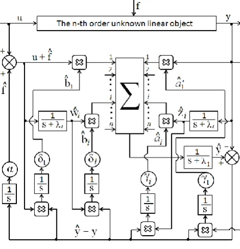
The block diagram of observer for identification of unknown parameters and external disturbance of plant showed in the Fig.1 is completely corresponded to the equations (3) – (6). In this scheme the place of action of the estimation 𝑓 of external disturbance is showed at the input of observer as 𝑢 + 𝑓 . Generally, in Eq. (4) the place of action of the estimation 𝑓 in observer should be defined in accordance with the place of action of the external disturbance f in the block diagram of plant.
Figure 1. Block diagram of adaptive observer
The signals of estimates of parameters 𝑎 1′, 𝑏 1, 𝑎 𝑖, 𝑏 𝑖
𝑖 = 2, 𝑛 and external disturbance 𝑓 of plant received at the outputs of corresponding integrators as well as the signals 𝑢, 𝑦, 𝑤𝑖 and 𝑧 𝑖 close the structure of observer
according to the Eq. (4). These closed contours of observer are self-adjustable on the identified values, i.e. in observer it is performed not only the identification of unknown parameters and external disturbance, but also the adaptation to their changes in process of functioning of plant. Therefore, the considered observer can be called the adaptive observer. At the same time by means of the corresponding choice of
amplification coefficients of integrators 𝛾𝑖, 𝛿𝑖 𝑖 = 1, 𝑛 , 𝛼
it is performed the optimisation of identification processes in order the estimation transitional processes in observer will be more quicker than transitional process in basic contour of control system.
The estimates of parameters 𝑎 1′, 𝑏 1, 𝑎 𝑖, 𝑏 𝑖 𝑖 = 2, 𝑛
and external disturbance 𝑓 of n-th order linear object being the output signals of corresponding integrators of adaptive observer can be used for formation of algorithms of control of linear objects with uncertain and/or changing parameters
𝑎1′, 𝑏1, 𝑎𝑖, 𝑏𝑖 𝑖 = 2, 𝑛 and disturbance f.
3. The Stability of Adaptive Observer
for Identification of Parameters and
Disturbance of Linear Object
Research the stability of plant by means of Lyapunov’s direct method. Let’s write the Eq. (3) for a plant in the following form:
𝑠𝑦 = 𝑎1𝑦 + 𝑎2𝑧2+ ⋯ + 𝑎𝑛𝑧𝑛+ 𝑏1 𝑢 + 𝑓 +
𝑏2 𝑤𝑢2+ 𝑤𝑓2 + ⋯ + 𝑏𝑛 𝑤𝑢𝑛 + 𝑤𝑓𝑛 , (8)
where
𝑤𝑢𝑖 =𝑠+𝜆1
𝑖𝑢, 𝑤𝑓𝑖 =
1
𝑠+𝜆𝑖𝑓, 𝑧𝑖 = 1
𝑠+𝜆𝑖𝑦, 𝑖 = 2, 𝑛
are the intermediate variables of plant.
This Eq. (8) it is possible also to obtain if the Eq. (1) of plant is represented in a canonical form as in [10] but with taking into account an external disturbance f:
𝑥 1
𝑥 2
⋮ 𝑥 𝑛
=
𝑎1 1 1 … 1
𝑎2
⋮ 𝑎𝑛
𝛬 𝑥1
𝑥2
⋮ 𝑥𝑛
+ 𝑏1
𝑏2
⋮ 𝑏𝑛
𝑢 + 𝑓 ,
𝑦1= 𝑥1, (9)
where 𝛬 is the 𝑛 − 1 × 𝑛 − 1 - diagonal matrix, which elements are the numbers −𝜆𝑖 𝑖 = 2, … , 𝑛 :
𝛬 =
−𝜆2 0 0 … 0
0 −𝜆3 0 … 0
…
0 …0 …0 …… … −𝜆𝑛
,
𝑎1, 𝑎2, … , 𝑎𝑛 Т= 𝑎 , 𝑏1, 𝑏2, … , 𝑏𝑛 Т= 𝑏 are the
parametric vectors.
Since a coordinate 𝑥1 is measured and is equal y, we can
write the Eq. (9) of plant in the following form:
𝑦
𝑥 ′ = 𝑎 𝑟 Т
𝛬 𝑦
𝑥 ′ + 𝑏 𝑢 + 𝑓 , (10)
where 𝑟Т= 1,1, … ,1 .
Let’s write the Eq. (4) for observer in the following form:
𝑠𝑦 = −𝜆1 𝑦 − 𝑦 + 𝑎 1𝑦 + 𝑎 2𝑧 2+ ⋯ + 𝑎 𝑛𝑧 𝑛+ 𝑏 1 𝑢 + 𝑓 +
𝑏 2 𝑤𝑢2+ 𝑤𝑓 2 + ⋯ + 𝑏 𝑛 𝑤𝑢𝑛 + 𝑤𝑓 𝑛 , (11)
where
𝑤𝑢𝑖 = 𝑤𝑢𝑖 =𝑠+𝜆1
𝑖𝑢, 𝑤𝑓 𝑖=
1
The same Eq. (11) it is possible to obtain if equations of observer are represented in the form as in [9] but with taking into account the estimate of external disturbance 𝑓 :
𝑤 = 𝛬′ Т𝑤 + 𝑟 𝑢 + 𝑓 ,′ 𝑦 𝑧 ′ = 𝑎 Т 𝑟 𝛬Т 𝑦
𝑧 + ′ 10 𝑏 Т𝑤 − 𝜆1𝑦 , (12)
where 𝑤 = 𝑢 + 𝑓 , 𝑤 ′Т
Т
, 𝑧 = 𝑦, 𝑧 ′Т
Т
and 𝑤 ′, 𝑧 ′ are 𝑛 − 1 – vectors of intermediate variables
𝑤2, 𝑤3, … , 𝑎 𝑛 Т= 𝑤𝑢2+ 𝑤𝑓 2, 𝑤𝑢3+ 𝑤𝑓 3, … , 𝑤𝑢𝑛+ 𝑤𝑓 𝑛
Т
and 𝑧 2, 𝑧 3, … , 𝑧 𝑛 Т of observer.
Let’s enter designations:
𝑎 = 𝑎 1, 𝑎 2, … , 𝑎 𝑛 Т= 𝑎 1, 𝑎 ′ Т Т
,
𝑏 = 𝑏 1, 𝑏 2, … , 𝑏 𝑛 Т
= 𝑏 1, 𝑏 ′ Т Т
,
𝑥 = 𝑥1, 𝑎 2𝑧 2+ 𝑏 2𝑤2, … , 𝑎 𝑖𝑧 𝑖+ 𝑏 𝑖𝑤𝑖 = 𝑦, 𝑥 ′ Т Т
. Let’s represent the Eq. (10) of plant in such form as the equation (12) of observer:
𝑤 = 𝛬𝑤 ′ ′+ 𝑟 𝑢 + 𝑓 , 𝑦 𝑧 ′ = 𝑎 Т 𝑟 𝛬Т 𝑦
𝑧 ′ + 10 𝑏 Т𝑤 , (13)
𝑤 = 𝑢 + 𝑓 , 𝑤 ′ Т Т, 𝑧 = 𝑦, 𝑧 ′ 𝑇 𝑇 and 𝑤 ′ = 𝑤 ′ 𝑢+
𝑤 ′
𝑓, 𝑧 ′ are 𝑛 − 1 – vectors of intermediate variables
𝑤2, 𝑤3, … , 𝑤𝑛 𝑇= 𝑤𝑢2+ 𝑤𝑓2, 𝑤𝑢3+ 𝑤𝑓3, … , 𝑤𝑢𝑛 + 𝑤𝑓𝑛
𝑇
and 𝑧2, 𝑧3, … , 𝑧𝑛 𝑇 of plant.
Subtract the Eq. (8) (or (13)) from the Eq. (11) (or (12)) with taking into account that 𝑧 𝑖 = 𝑧𝑖 and 𝑤𝑢𝑖 = 𝑤𝑢𝑖:
𝑦 = −𝜆1𝑦 + 𝑎 1− 𝑎1 𝑦 + 𝑎 − 𝑎 ′ ′ Т
𝑧 ′+ 𝑏
1− 𝑏1 𝑢 +
𝑏 1𝑓 − 𝑏1𝑓 + 𝑏 − 𝑏 ′ ′ 𝑇
𝑤 ′
𝑢+ 𝑛𝑖=2 𝑏 𝑖𝑤𝑓 𝑖− 𝑏𝑖𝑤𝑓𝑖 . (14)
Consider a positive-definite square function of Lyapunov in the following form:
𝑉 =12𝑦 2+1 2 1 𝛾𝑖 𝑎 𝑖− 𝑎𝑖 2 𝑛 𝑖=1 + 1 2 1 𝛿𝑖 𝑏 𝑖− 𝑏𝑖 2 𝑛 𝑖=1 + 𝑏1
2𝛼 𝑓 − 𝑓 2
+12 𝑠+𝜆𝑖 𝑏𝑖
𝛼 𝑤𝑓 𝑖− 𝑤𝑓𝑖 2 𝑛
𝑖=2 . (15)
Let’s write a full derivative of this Eq. (15):
𝑉 = 𝑦 𝑦 + 1 𝛾𝑖 𝑛 𝑖=1 𝑎 𝑖− 𝑎𝑖 𝑎 𝑖 + 1 𝛿𝑖 𝑛 𝑖=1 𝑏 𝑖− 𝑏𝑖 𝑏 𝑖 + 𝑏1 𝛼 𝑓 − 𝑓 𝑓 + + 𝑠+𝜆𝑖 𝑏𝑖 𝛼 𝑛
𝑖=2 𝑤𝑓 𝑖− 𝑤𝑓𝑖 𝑤 𝑓 𝑖, (16)
where 𝑤 𝑓 𝑖 = 1 𝑠+𝜆𝑖𝑓 =
−𝛼 𝑠+𝜆𝑖𝑦 .
Eq. (16) of a derivative 𝑉 according to the observer equations (5), (6) and the deviation Eq. (14) has the same result as in [10]:
𝑉 = 𝑦 𝑦 + 𝛾1
𝑖
𝑛
𝑖=1 𝑎 𝑖− 𝑎𝑖 𝑎 𝑖 + 𝛿1
𝑖
𝑛
𝑖=1 𝑏 𝑖− 𝑏𝑖 𝑏 𝑖 + 1
𝛼 𝑛
𝑖=1 𝑓 − 𝑓 𝑓 = −𝜆1𝑦 2. (17)
This obtained result of Eq. (17) is proved that the estimated in observer variables 𝑎 𝑖, 𝑏 𝑖, 𝑓 asymptotically
converge to their real values 𝑎𝑖, 𝑏𝑖, 𝑓 𝑖 = 1, 𝑛 in plant.
A speed of convergence depends of coefficients of integrators 𝛾𝑖, 𝛿𝑖 and 𝛼. At the same time on the basis of a
hypothesis of quasistationarity [11,12] it is supposed that during transition processes in observer variables 𝑎𝑖, 𝑏𝑖, 𝑓
𝑖 = 1, 𝑛 in plant do not change.
4. Design of Adaptive Observer for
Identification of Linear Model of DC
Electric Drive with Variable Load
Consider the application of adaptive observer described by the equations (4) – (6) for a linear object with disturbance. As such linear object could be considered a linear model of the electric drive in mobility degree of the multilink manipulator robot (MR) being the joint drive with a variable mechanical load [13-15].
The equation of moments on a shaft of the direct current (dc) electric motor:
𝐽𝑠𝜔m= Мm− 𝑀, (18)
where 𝐽 = 𝐽 𝑞 , 𝜉 is the moment of inertia of drive load changing in dependence on a vector 𝑞 of generalized coordinates and a vector 𝜉 of parameters of MR and its payload (geometrical, weight-inertial parameters, etc.) [16], i.e. is the unknown parameter of plant; 𝑀 = 𝑀 𝑞 , 𝑞 , 𝜉 is counted to a shaft of motor the torque of resistance of the drive load which changes are caused by mutual influence of movements on degrees of mobility of MR, moments from the gravity of links and a payload of MR, etc. [16], i.e. is the external disturbing signal for a plant; М𝑚 = 𝑘m𝑖𝑎 is the
torque of dc motor in which 𝑘𝑚 is the motor’s torque
constant, 𝑖𝑎 is the armature current being the input signal
for a plant; 𝜔𝑚 is the speed of rotation of the shaft of motor
being the output signal for a plant; 𝑠 = 𝑑 𝑑𝑡 is the differentiation operator.
Let’s represent the Eq. (18) of plant in the following form:
𝜔𝑚 =𝐽s1 𝑘m𝑖𝑎− 𝑀 . (19)
According to the Eq. (2) the Eq. (19) of plant is written in the following form:
𝑦 =𝑏1 𝑢+𝑓
𝑠 , (20)
where 𝑢 = М𝑚 = 𝑘m𝑖𝑎 is the input signal of plant
measured by means of the armature current sensor with a transfer coefficient 𝑘𝑐; 𝑦 = 𝑘s𝜔𝑚 is the output signal of
plant measured by means of the speed sensor with a transfer coefficient 𝑘s; 𝑏1= 1 𝐽 is the unknown parameter of
a)
b)
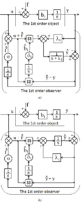
Figure 2. Block diagrams of observer for the 1st order object
On the basis of the measured input М𝑚 and output 𝜔𝑚
signals of plant (18)-(20) and according to the basic provisions of design of observer stated above it is necessary to estimate the unknown values of parameter 1 𝐽 and external disturbance M of the considered plant.
Since the Eq. (20) has the 1st order the equation for 1st order observer obtained on the Eq. (4) at 𝑎𝑖 = 0 𝑖 = 1, 𝑛 ,
𝑏𝑖 = 0 𝑖 = 2, 𝑛 has the following form:
𝑦 =𝑠+𝜆1
1 𝑏 1 𝑢 + 𝑓 + 𝜆1𝑦 , (21)
where 𝑦 = 𝑘s𝜔m is the estimate of output signal 𝑦 equal
to the estimate of angular velocity of the shaft of motor 𝜔m
with a transfer coefficient 𝑘𝑠; 𝑏 1= 1 𝐽 is the estimate of
unknown parameter 𝑏1, in which 1 𝐽 is the inverse value
of the estimate 𝐽 of unknown moment of inertia of drive load; 𝑓 = −𝑀 is the estimate of the external disturbance being the estimate of the torque of resistance of drive load.
Estimates of the parameter 𝑏 1 and disturbance 𝑓 are
formed at the outputs of corresponding integrators
according to equations (5), (6) by the following formulas:
𝑏 1= −𝛿1 𝑢 + 𝑓 𝑦 1, 𝑓 1 = −𝛼𝑦 1
or 𝑏 1=−𝛿1 𝑢+𝑓 𝑦 𝑠 1, 𝑓 1=−𝛼𝑦 𝑠1, (22)
where 1 𝑠 is the integration operator.
The block diagram of observer for the considered 1st order plant corresponding to the equations (21), (22) is showed in the Fig. 2,a. Let’s transform this scheme to the
form showed in the Fig. 2,b conforming more to the model of plant (19).
Let’s represent the block diagrams of the 1st
order plant and its observer showed in the Fig. 2,b with taking into account designations of variables of electric drive in the equations (18), (19), (21), (22). The obtained block diagrams of the “mechanical” part of electric drive and its observer are showed in the Fig. 3.
Figure 3. Block diagrams of 1st order plant and its observer
5. The Stability of Adaptive Observer
for Identification of Parameter and
Disturbance of Electric Drive
For obtaining the estimate 𝐽 of moment of inertia J and the estimate 𝑀 of torque of resistance M of mechanical load of electric drive the algorithm of operating of adaptive observer according to the block diagram in the Fig. 3 has the following form [17]:
𝑑 1 𝐽 𝑑𝑡 = 𝛿1 𝑀𝑚− 𝑀 𝑘𝑠 𝜔𝑚− 𝜔𝑚 ,
𝑑𝜔𝑚 𝑑𝑡= 1 𝐽 𝑀𝑚− 𝑀 + 𝜆1𝑘𝑠 𝜔𝑚− 𝜔𝑚 ,
𝑑𝑀 𝑑𝑡= −𝛼𝑘𝑠 𝜔𝑚− 𝜔𝑚 (23)
with the initial conditions:
𝜔𝑚 0 = 0, 𝐽 −1 0 = 𝐽0−1, 𝑀 0 = 0,
where 𝐽0 is the average value from the possible range of
changes of moment of inertia J.
Consider the stability of the adaptive observer for identification of 𝐽−1 and 𝑀 variables. Let’s use the following designations:
and take into account that
𝑠𝜔𝑚 = 𝜔 𝑚 = 𝑑𝜔𝑚 𝑑𝑡= 1 𝐽 𝑀𝑚− 𝑀 ,
then the operation algorithm of the adaptive observer in e, 𝜈 and 𝜇 coordinates can be described by the equations:
𝑑𝑒 𝑑𝑡= 1 𝐽 𝑀𝑚− 𝑀 −
1 𝐽 𝑀𝑚− 𝑀 − 𝜆1𝑘𝑠𝑒,
𝑑𝜈 𝑑𝑡= −𝛿1 𝑀𝑚− 𝑀 𝑘𝑠𝑒,
𝑑𝜇 𝑑𝑡= 𝛼𝑘𝑠𝑒. (24)
At the same time we will accept initial conditions:
𝑒 0 = 0, 𝜈 0 = 𝐽−1− 𝐽0−1, 𝜇 0 = 0,
and on the basis of a hypothesis of quasistationarity [11,12] we’ll consider that on the time interval corresponding to transition process in observer the variables 𝐽−1 and 𝑀 do not change.
Let’s prove that the position of balance of system of the equations (24) is asymptotically stable, i.e.
lim𝑡→∞𝑒 = 0, lim𝑡→∞𝜈 = 0, lim𝑡→∞𝜇 = 0.
Let’s consider a positive-definite Lyapunov’s function of a following form:
𝑉 =12𝑒2+ 1 2𝛿1𝑘𝑠𝜈
2+ 1
2𝛼𝑘𝑠𝐽𝜇
2, (25)
where 𝐽 = 𝑐𝑜𝑛𝑠𝑡 - because it corresponds to a quasistationarity interval.
Considering that
𝜇 = 𝑀 − 𝑀 = 𝑀𝑚 − 𝑀 − 𝑀𝑚 − 𝑀 ,
Let's write down a full derivative of Eq. (25) with respect to time on the basis of system of the equations (24):
𝑑𝑉 𝑑𝑡= −𝜆1𝑘𝑠𝑒2. (26)
According to Eq. (26) the result of a full derivative of Lyapunov’s function is negative and the operating of adaptive observer described by the equations (23) is stable. Let's show that at 𝑒 ≡ 0 there are also 𝜈 ≡ 0 and 𝜇 ≡ 0. For this purpose we will consider at 𝑒 ≡ 0 the system of equations (24):
0 = 1 𝐽 𝑀𝑚− 𝑀 − 1 J 𝑀𝑚− 𝑀 ,
𝑑𝜈 𝑑𝑡= 0, 𝑑𝜇 𝑑𝑡= 0.
The equality to zero of the first equation means
1 𝐽 = 1 𝐽 and 𝑀 = 𝑀, therefore at 𝑒 ≡ 0 the identical equality to zero of 𝜈 = 1 𝐽 − 1 𝐽 and 𝜇 = 𝑀 − 𝑀 parameters are obviously. Therefore, the function 𝑑𝑉 𝑑𝑡 is negative-definite and if the identification observer would be constructed according to equations (23) the 1 𝐽 and 𝑀 estimates would asymptotically approach to their actual values of the moment of inertia 1 𝐽 and the torque of resistance M of load of the drive. The convergence of process of estimate depends on 𝜆1, 𝛿1 and 𝛼 coefficients,
which can be practically always chosen from a condition that the estimation processes in adaptive observer be occurred quicker than the main transition process in control system of the drive.
6. Simulation Results of Control System
with Adaptive Observer for
Identification of Parameter and
Disturbance
In addition to the Eq. (16) of plant let’s write the following equations for forming of control signal [15,18]:
𝑢𝑎= 𝑖𝑎𝑅𝑎+ 𝑘𝜔𝜔𝑚, 𝑢 = 𝑘𝑢𝑎, (27)
where 𝑢𝑎 and 𝑅𝑎 are the armature voltage and the
armature resistance of electric motor; 𝑘𝜔 is the motor’s
back-emf constant; 𝑢 and 𝑘 are the control signal and the amplification coefficient of power amplifier of drive.
Taking into account the equations (27) it is possible to write the Eq. (19) of plant in following form:
𝐽𝜔 𝑚+ 𝑘𝑚𝑘𝜔𝑅𝑎−1𝜔𝑚 = 𝑘𝑚𝑘𝑅𝑎−1𝑢 − 𝑀, (28)
where 𝐽 and 𝑀 are the unknown variables.
Let the control signal of drive has the following form [19,20]:
𝑢 = 𝑢 𝜑, 𝜔𝑚, 𝐽 , 𝑀 = (𝑘𝑝𝑘1 𝜑∗− 𝜑 −
𝑘𝑠𝑘2𝜔𝑚)𝐽 + 𝑘𝑠𝑘3𝜔𝑚+ 𝑘4𝑀, (29)
where 𝜑∗ and 𝜑 are respectively the demand and the actual angular positions of an output shaft of the drive; 𝑘𝑝 is
the transfer coefficient of sensor of angular position of a shaft of the drive; 𝑘1, 𝑘2, 𝑘3, 𝑘4 are the constant
parameters selected so, that at 𝐽 = 𝐽0= 𝑐𝑜𝑛𝑠𝑡 and 𝑀 = 0
set in model of the drive (28), the desirable transition process of control system at 𝜑∗ 𝑡 = 1 𝑡 will have the set duration 𝑇, s and the set overshoot 𝜎, %; 𝐽 = 𝐽 −1 and 𝑀 are the estimates received in observer on the equations (23). In the program of simulation the different values of the moment of inertia 𝐽 and the external torque 𝑀 of load are set in the Eq. (28), these given values of load are estimated in observer on an algorithm (23) and used for formation of a control algorithm (29) [19, 20]. Results of simulation of dynamics of control of a rotation link drive of MR at variable values of mechanical load are given in Figures 4, 5 and 6.
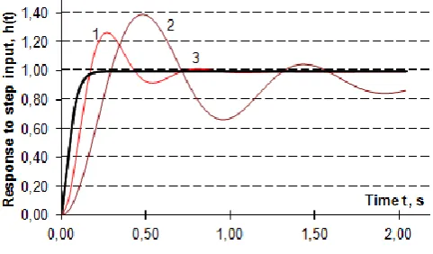
1 - system without observer at 𝐽=7 kg*m2 and 𝑀=10 N*m; 2 – system without observer at 𝐽=25 kg*m2 and 𝑀=100 N*m; 3 – system with observer at the same values of 𝐽 and 𝑀 of load
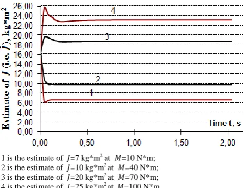
1 is the estimate of 𝐽=7 kg*m2 at 𝑀=10 N*m; 2 is the estimate of 𝐽=10 kg*m2 at 𝑀=40 N*m; 3 is the estimate of 𝐽=20 kg*m2 at 𝑀=70 N*m; 4 is the estimate of 𝐽=25 kg*m2 at 𝑀=100 N*m.
Figure 5. Transition processes of identification of the moment of inertia of load
1 is the estimate of 𝑀=10 N*m at 𝐽=7 kg*m2; 2 is the estimate of 𝑀=40 N*m at 𝐽=10 kg*m2; 3 is the estimate of 𝐽=20 kg*m2 at 𝑀=70 N*m; 4 is the estimate of 𝑀=70 N*m at 𝐽=25 kg*m2.
Figure 6. Transition processes of identification of the external torque of load
The desirable transition process is chosen aperiodic (monotonous) (Fig. 4, the curve 3). Setting various values of the moment of inertia J and the external torque M of load in model of the drive (28) with the not adaptive to a load control algorithm (in Eq. (29) 𝐽 = 𝐽0= 𝑐𝑜𝑛𝑠𝑡 and 𝑀 = 0)
it is possible to see that to increase in the values of J and M
there is a deterioration in characteristics of transitional functions ℎ 𝑡 = 𝜑 𝑡 (duration, overshoot and steady-state error increase) - in the Fig. 4, the curves 1 and 2. While in control system with observer at these different values of mechanical load the characteristics of transitional functions don't change (the Fig. 4, a curve 3), i.e. independent of changes of load in control system with observer the set duration and overshoot of desired transition process always take place, and the steady-state error of the control system is completely eliminated.
The graphs in Figures 4, 5, 6 of transition processes in observer at the identification of different values of the moment of inertia J and the external torque M of load set in model of the drive (28) have shown that the use of the values J and M estimated in observer to form an adaptive
control algorithm (29) provides the invariable characteristics of transitional functions in the control system, i.e. independent of changes of mechanical drive load in control system with observer the desirable transition process - a curve 3 in the Fig. 4 always takes place.
In the Figures 5, 6 are shown curves 1 - 4 of transition processes in observer at the identification of unknown values of the moments of inertia J and the external torques of load M set in the drive model (28). From curves in Figures 4, 5 and 6 it is also visible that process of estimation of unknown variables of the moments of inertia J
happens quicker than transition process in the main contour of control system, that is necessary for the stable work of a load adaptive control system of the drive, and the estimated values of the unknown external torques M of load eliminate a steady-state error of the drive.
7. Conclusions
In the paper the known procedure of synthesis of adaptive observer for identification of parameters and state coordinates of linear object is considered taking into account the identification of the scalar external disturbance operating on control object. In the block diagram of adaptive observer the place of action of the estimation 𝑓 of external disturbance is showed at the input of observer and the obtained observer provides asymptotic stability of processes for identification of parameters and external disturbance of object. Generally, the place of action of the estimation 𝑓 in observer should be defined in accordance with the place of action of the external disturbance f in the block diagram of control object. Using considered in the paper technique it is possible to design the adaptive observer and prove its asymptotic stability of processes for identification of parameters and an external disturbance for other physical linear control objects (plants).
An example of use of the proposed adaptive observer for linear model of the dc electric drive with the variable mechanical load is showed that the processes for identification of the moment of inertia and the torque of resistance of drive load, i.e. the processes for identification of the uncertain parameter and an external disturbance of linear object are carried out simultaneously (concurrently, joint). Asymptotic stability of identification processes of uncertain parameter and external disturbance is proved. Received results of identification and their use for adaptation of an example of linear object are shown on graphs of transition processes and provide adaptive stabilization of desirable dynamic properties of considered control system.
REFERENCES
[2] Zhong, Q.S. and Rees, D. “Control of uncertain lti systems based on an uncertainty and disturbance estimator”, Journal of Dynamics Systems, Measurement and Control, 2004, 126(4), pp.905-910.
[3] Guo, B.Z. and Zhao, Z.I. “On the convergence of an extended state observer for nonlinear systems with uncertainty”, Systems@Control Letters, 2011, 60(6), pp.420-430. [4] She, J.H, Xin X. and Pan Y. “Equivalent-input-disturbance
approach - Analyses and application to disturbance rejection in dual-stage feed drive control systems”, IEEE/ASME Transactions on Mechatronics, 2011, 16(2), pp.330-340. [5] Jo, N.H., Joo, Y. and Shim, H. “A study of disturbance
observers with unknown relative degree of the plant”, Automatica, 2014, 50(6), pp.1730-1734.
[6] Huang, Y. and Xue, W. “Active disturbance rejection control: methodology theoretical and analyses”, ISA Transactions, 2014, 53(4), pp.963-976.
[7] Chen W.-H., Yang, J., Guo, L. and Li, S. “Disturbance observer based control and related methods: an overview”, IEEE Transactions on industrial electronics, 2016, 63(2), pp.1083-1095.
[8] P. Eykhoff, Bases of identification of control systems: parameter and state estimation, Moscow, Russia: Mir, 1975. (In Russ.)
[9] G. Luders, K.S. Narendra, “A new canonical form for an adaptive observes”, IEEE Transactions on automatic control, April, 1974, pp.117-119.
[10] N. T. Kuzovkov, Modal control and the observing devices, Moscow, Russia: Mashinostrojenie, 1976. (In Russ.)
[11] A. V. Basharin, V. A. Novikov, G. G. Sokolovskij, Control of electric drives, Leningrad, Russia: Energoizdat. Leningradskoje otdelenije, 1982. (In Russ.)
[12] A. G. Alexandrov, Optimum and adaptive systems, Moscow, Russia: Vysshaya shkola, 1989. (In Russ.)
[13] J. J. Craig, Introduction to robotics: Mechanics and Control, Upper Saddle River, New Jersey: Pearson Education, Inc., 2005.
[14] F. L. Lewis, D. M. Dawson, C. T. Abdallah, Robot Manipulator Control: Theory and Practice, New York, Basel: Marcel Decker, Inc., 2004.
[15] S. F. Burdakov, V. A. Dyachenko, A. N. Timofeev, Design of manipulators of industrial robots and robotic complexes, Moscow: Vyssh. Shkola, 1986. (In Russ.)
[16] Dynamics of control of robots, Under E. I. Yurevich's edition. Moscow: Science, 1984. (In Russ.)
[17] B. K. Kussainov, “Adaptive control system of the robot drive”, Proceedings of the International Forum "Science and Engineering Education without Borders", Almaty: KazNTU named after K.I. Satpayev, Vol.2, pp. 352-355, 2009. (In Russ.)
[18] N. Mohan, Electric Drives: An Integrative Approatch, Minneapolis: MNPERE, 2003.
[19] B. Kussainov, “A load adaptive control system of manipulator robot’s drive” International Scientific Journal “Innovations”. Year VI, Issue 3, pp. 78-81, 2018.