Classification of Motor Imagery Using Combination of Feature Extraction and Reduction Methods for Brain-Computer Interface

(1)

225

Information Technology and Control 2019/2/48

Classification of Motor Imagery

Using Combination of Feature

Extraction and Reduction Methods

for Brain-Computer Interface

ITC 2/48

Journal of Information Technology and Control

Vol. 48 / No. 2 / 2019 pp. 225-234

DOI 10.5755/j01.itc.48.2.23091

Classification of Motor Imagery Using Combination of Feature Extraction and Reduction Methods for Brain-Computer Interface

Received 2019/04/05 Accepted after revision 2019/05/15

http://dx.doi.org/10.5755/j01.itc.48.2.23091

Corresponding author: [email protected]

Vacius Jusas

Department of Software Engineering; Kaunas University of Technology; Kaunas, Lithuania; e-mail: [email protected]

Sam Gilvine Samuvel

Department of Software Engineering; Kaunas University of Technology; Kaunas, Lithuania; e-mail: [email protected]

The motor imagery (MI) based brain-computer interface systems (BCIs) can help with new communication ways. A typical electroencephalography (EEG)-based BCI system consists of several components including signal acquisition, signal pre-processing, feature extraction and feature classification. This paper focuses on the feature extraction step and proposes to use a combination of several feature extraction and feature reduc-tion methods. The research presented in the paper explores the methods of band power, time domain param-eters, fast Fourier transform and channel variance for feature extraction. These methods are investigated by combining them in pairs. The application of two feature extraction methods increases the number of selected features that can be redundant or irrelevant. The utilization of too many features can lead to wrong classifica-tion results. Therefore, the methods of feature reducclassifica-tion have to be applied. The following feature reducclassifica-tion methods are investigated: principal component analysis, sequential forward selection, sequential backward selection, locality preserving projections and local Fisher discriminant analysis. The combination of the meth-ods of fast Fourier transform, channel variance and principal component analysis performed the best among the combinations of methods. The obtained classification accuracy of the above-mentioned combination of the methods is much higher than that of the individual feature extraction method. The novelty of the approach is based on consolidated sequence of methods for feature extraction and feature reduction.

(2)

226

1. Introduction

The analysis based on the electroencephalograph (EEG) records provides valuable information on the brain activities. The mental activities guide the changes in the brain’s signals. The BCI framework is responsible for acquiring, measuring, and convert-ing these brain signals into control commands. As a non-invasive measurement method of brain activ-ity, EEG has attracted increasing interest because of its low risk, low cost, and significant potential for practical applications. EEG data are generally com-posed of multichannel signals recorded from several electrodes placed on the scalp to record the activity of various cortexes. The decoding of human motor intentions mainly utilizes motor imagery (MI) EEG signals and could provide users with direct control of various devices without utilizing any

peripheral nerves or muscle movements [6, 13]. The typical EEG-based BCI framework consists of sev-eral components, such as signal acquisition, signal pre-processing, feature extraction and feature clas-sification. The component of feature extraction has a direct influence on the success of feature classifica-tion. Therefore, the methods of feature extraction are very important and of huge interest to the research-ers. EEG is a type of random signal that contains highly complex information. Thus, a single feature extraction method usually cannot describe the prop-erties of EEG signals fully. So, it is necessary to take full advantage of different types of feature extraction methods and explore the optimal combination of input features. While several methods are combined to extract features from original EEG signals, the problem of dimensionality appears. Moreover, many extracted features might be redundant or irrelevant; consequently, they can have a negative effect on clas-sification task. In this case, a dimensionality reduc-tion becomes an important preprocessing step before feature classification.

This paper presents the efficient feature extraction approach for EEG signals classification and suggests utilizing a combination of several methods for feature extraction and reduction. The combination of several methods of feature extraction and reduction can well express the different characteristics of EEG signals. The paper is organized as follows: Section 2 focuses on the related work, Section 3 presents the methods

used in this research, Section 4 introduces our pro-posed approach. The experimental results are deliv-ered in Section 5 and Conclusions form Section 6.

2. Related Work

Rodriguez-Bermudez et al. [17] presented a wrap-per-based methodology for feature selection. Fea-tures are computed in different time segments using feature extraction methods for power spectral densi-ty (PSD) features, adaptive autoregressive (AAR) co-efficients and Hjorth parameters. The features then are averaged and concatenated into a single vector. Next, the proposed framework is used to select the appropriate features. The framework has two stages. The first stage involves feature ranking and the sec-ond stage consists in the selection of the most suit-able features utilizing a leave-one-out estimation based on the Allen’s PRESS statistics. Two different procedures have been considered for feature ranking, such as least angle regression (LARS) and the Wilcox-on rank sum test. It is cWilcox-onfirmed that the LARS algo-rithm provides better results than the Wilcoxon rank sum test. The experiment showed that PSD features are the most selected in all the cases; next, the Hjorth parameters; and the less informative variables corre-spond to the AAR coefficients.

(3)

227

the classifier performance with respect to the origi-nal feature space. It has been noticed that the LFDA showed the best results for all subjects with reduced computational complexity.

Yu et al. [23] analyzed the performance of the feature ex-traction method using the following spatial filter tech-niques: common average reference, common spatial pattern, no-spatial filter and feature reduction method using principle component analysis. The results of the experiment showed that the common average reference filter had a better performance than other universal spatial filter techniques. The feature reduction method of principal component analysis did not improve ac-curacy but maintained the classification performance while decreasing feature number effectively.

Gupta et al. [9] considered empirical mode decompo-sition and wavelet transform for feature extraction. To decrease the size of the feature vector, six multi-variate filter methods such as Euclidean distance, Bhattacharyya distance measure, Kullback-Leibler distance, ratio of scatter matrices, linear regression and minimum redundancy-maximum relevance were investigated. For all the multivariate filter methods, the top 25 features were incrementally included one by one to develop the decision model using sequen-tial forward selection search method. Experimental results showed that the classification accuracy im-proved with the use of each of the six multivariate feature selection methods. Among all the investigat-ed combinations of feature extraction and selection methods, the combination of wavelet transform and linear regression performed the best.

Ren et al. [16] proposed a feature extraction framework that combined hybrid feature extraction and feature selection method. The following feature extraction methods of different types were applied: autoregres-sive model, discrete wavelet transform, wavelet packet transform and sample entropy. The hybrid input fea-ture vector was composed of 83 feafea-tures. For feafea-ture selection, algorithms of minimal redundancy-maxi-mal relevance and Fisher score based on global search strategy were used. For comparison purposes, the fea-ture reduction method of principal component analy-sis was introduced. The experimental results demon-strated that class separability was not improved after transformation utilizing principal component analy-sis. The hybrid features selected on the basis of Fisher score yielded the highest classification accuracy.

Baig et al. [2] implemented a hybrid method that used common spatial patterns filter to extract feature space, then used the method of differential evolution with a classifier (wrapper) to discover the optimized feature subset. The Authors also implemented the following evolutionary algorithms: particle swarm optimization, simulated annealing, ant colony opti-mization, and artificial bee colony. The experimental results demonstrated that the proposed hybrid meth-od performed well with classifier of support vector machine. Moreover, the comparison results of imple-mented evolutionary algorithms showed the superi-ority of the method of differential evolution. However, the proposed method is slow compared to the typical feature selection algorithms and the classifier of the wrapper technique makes it even slower.

Zhang et al. [25] combined autoregressive model and sample entropy for the feature extraction. Each fea-ture vector acquired on the basis of the combination strategy contained two parts: autoregressive coeffi-cients and sample entropy values. In the classifica-tion stage, the authors utilized support vector ma-chine with radial basis function (RBF) kernel as the classifier. Experimental results showed that the com-bination strategy of the feature extraction obtained a better accuracy in comparison with autoregressive model-based method.

(4)

228

3. Methods

In this section, we are presenting all methods which will be applied in the experiments. First of these methods is a common spatial pattern which will be used for pre-processing. The inclusion of the pre-pro-cessing stage is an important procedure due to the high variability of the EEG measurements [1].

3.1. Common Spatial Patterns

The common spatial pattern technique was initial-ly proposed for classification of multi-channel EEG during imagined hand movements by Ramoser et al. [15]. The primary idea is to utilize a linear transform to project. The multi-channel EEG data into a low di-mensional spatial subspace with a projection matrix, whose every row comprises of weights for channels. This change can augment the variance of two class signal matrices. CSP method depends on the concur-rent diagonalization of the covariance matrices of two classes.

The points of the algorithm are described as follows with the case of characterizing single preliminary EEG during hand and foot movements XH and XF namely

the preprocessed EEG matrices under two conditions (hand and foot) with dimensions N*T, where N is the number of channels and T is the number of samples per channel [22]. The standardized spatial covariance of the EEG can be represented as follows:

hybrid features selected on the basis of Fisher score yielded the highest classification accuracy.

Baig et al. [2] implemented a hybrid method that used common spatial patterns filter to extract feature space, then used the method of differential evolution with a classifier (wrapper) to discover the optimized feature subset. The Authors also implemented the following evolutionary algorithms: particle swarm optimization, simulated annealing, ant colony optimization, and artificial bee colony. The experimental results demonstrated that the proposed hybrid method performed well with classifier of support vector machine. Moreover, the comparison results of implemented evolutionary algorithms showed the superiority of the method of differential evolution. However, the proposed method is slow compared to the typical feature selection algorithms and the classifier of the wrapper technique makes it even slower.

Zhang et al. [25] combined autoregressive model and sample entropy for the feature extraction. Each feature vector acquired on the basis of the combination strategy contained two parts: autoregressive coefficients and sample entropy values. In the classification stage, the authors utilized support vector machine with radial basis function (RBF) kernel as the classifier. Experimental results showed that the combination strategy of the feature extraction obtained a better accuracy in comparison with autoregressive model-based method.

Han et al. [10] proposed an EEG classification framework based on EEG feature compression and convergent iterative channel positioning. The framework begins with an EEG signal pre-processing and single channel based on autoregressive coefficients or time domain parameters feature extraction. Next, after dividing all the trials into the training and testing sets, all the features from the different channels for the training trials are gathered and cluster signatures assigned to them through k-means. Then, EEG signals are mapped from the three-dimensional matrix (trial channel-feature) to a two-dimensional (trial-channel) matrix by compressing all feature vectors into their cluster signatures. For the two-dimensional matrix, RFS, RUFS, or SSLSR methods to rank and select the channels are employed. The results of the experiment showed that the execution of the proposed system is comparable with the state-of-the-art techniques. In the experiment, they performed only two motor imagery tasks. In this research, we used a four different motor imagery tasks.

3. Methods

In this section, we are presenting all methods which will be applied in the experiments. First of these methods is a common spatial pattern which will be used for pre-processing. The inclusion of the pre-processing stage is an important procedure due to the high variability of the EEG measurements [1].

3.1. Common Spatial Patterns

The common spatial pattern technique was initially proposed for classification of multi-channel EEG during imagined hand movements by Ramoser et al. [15]. The primary idea is to utilize a linear transform to project. The multi-channel EEG data into a low dimensional spatial subspace with a projection matrix, whose every row comprises of weights for channels. This change can augment the variance of two class signal matrices. CSP method depends on the concurrent diagonalization of the covariance matrices of two classes.

The points of the algorithm are described as follows with the case of characterizing single preliminary EEG during hand and foot movements XH and XF namely the preprocessed EEG matrices under two conditions (hand and foot) with dimensions N*T, where N is the number of channels and T is the number of samples per channel [22]. The standardized spatial covariance of the EEG can be represented as follows:

( ) / ( ( )),

( ) / ( ( )).

T T

H H H H H

T T

F F F F F

R X X trace X X R X X trace X X

=

= (1)

3.2 . Feature Extraction

3.2.1. Band Power

There exist various methods for band power (BP) feature extraction from EEG signals. In this investigation, we used a method implemented in the Biosig biomedical signal processing library that enumerates the band power by band-pass filtering the signal [18]. According to this method, initially, the signal is filtered through a band-pass filter that is designed for a given frequency band. In case of a Biosig library, a 4th order Butterworth infinite impulse response (IIR) filter is used. The next step consists in squaring each sample of the resulting signal 𝑥𝑥𝑥𝑥(𝑡𝑡𝑡𝑡)1_{, which contains only the}

required frequency components, to achieve the time course of power

2_{( ).}

p x t= (2)

(1)

3.2. Feature Extraction

3.2.1. Band Power

There exist various methods for band power (BP) fea-ture extraction from EEG signals. In this investiga-tion, we used a method implemented in the Biosig bio-medical signal processing library that enumerates the band power by band-pass filtering the signal [18]. Ac-cording to this method, initially, the signal is filtered through a band-pass filter that is designed for a given frequency band. In case of a Biosig library, a 4th order Butterworth infinite impulse response (IIR) filter is used. The next step consists in squaring each sample of the resulting signal x(t)1_{, which contains only the}

required frequency components, to achieve the time course of power

hybrid features selected on the basis of Fisher score yielded the highest classification accuracy.

Baig et al. [2] implemented a hybrid method that used common spatial patterns filter to extract feature space, then used the method of differential evolution with a classifier (wrapper) to discover the optimized feature subset. The Authors also implemented the following evolutionary algorithms: particle swarm optimization, simulated annealing, ant colony optimization, and artificial bee colony. The experimental results demonstrated that the proposed hybrid method performed well with classifier of support vector machine. Moreover, the comparison results of implemented evolutionary algorithms showed the superiority of the method of differential evolution. However, the proposed method is slow compared to the typical feature selection algorithms and the classifier of the wrapper technique makes it even slower.

Zhang et al. [25] combined autoregressive model and sample entropy for the feature extraction. Each feature vector acquired on the basis of the combination strategy contained two parts: autoregressive coefficients and sample entropy values. In the classification stage, the authors utilized support vector machine with radial basis function (RBF) kernel as the classifier. Experimental results showed that the combination strategy of the feature extraction obtained a better accuracy in comparison with autoregressive model-based method.

Han et al. [10] proposed an EEG classification framework based on EEG feature compression and convergent iterative channel positioning. The framework begins with an EEG signal pre-processing and single channel based on autoregressive coefficients or time domain parameters feature extraction. Next, after dividing all the trials into the training and testing sets, all the features from the different channels for the training trials are gathered and cluster signatures assigned to them through k-means. Then, EEG signals are mapped from the three-dimensional matrix (trial channel-feature) to a two-dimensional (trial-channel) matrix by compressing all feature vectors into their cluster signatures. For the two-dimensional matrix, RFS, RUFS, or SSLSR methods to rank and select the channels are employed. The results of the experiment showed that the execution of the proposed system is comparable with the state-of-the-art techniques. In the experiment, they performed only two motor imagery tasks. In this research, we used a four different motor imagery tasks.

3. Methods

In this section, we are presenting all methods which will be applied in the experiments. First of these methods is a common spatial pattern which will be used for pre-processing. The inclusion of the pre-processing stage is an important procedure due to the high variability of the EEG measurements [1].

3.1. Common Spatial Patterns

The common spatial pattern technique was initially proposed for classification of multi-channel EEG during imagined hand movements by Ramoser et al. [15]. The primary idea is to utilize a linear transform to project. The multi-channel EEG data into a low dimensional spatial subspace with a projection matrix, whose every row comprises of weights for channels. This change can augment the variance of two class signal matrices. CSP method depends on the concurrent diagonalization of the covariance matrices of two classes.

The points of the algorithm are described as follows with the case of characterizing single preliminary EEG during hand and foot movements XH and XF namely the preprocessed

EEG matrices under two conditions (hand and foot) with dimensions N*T, where N is the number of channels and T is the number of samples per channel [22]. The standardized spatial covariance of the EEG can be represented as follows:

( ) / ( ( )),

( ) / ( ( )).

T T

H H H H H

T T

F F F F F

R X X trace X X

=

= (1)

3.2. Feature Extraction 3.2.1. Band Power

There exist various methods for band power (BP) feature extraction from EEG signals. In this investigation, we used a method implemented in the Biosig biomedical signal processing library that enumerates the band power by band-pass filtering the signal [18]. According to this method, initially, the signal is filtered through a band-pass filter that is designed for a given frequency band. In case of a Biosig library, a 4th order Butterworth infinite impulse response (IIR) filter is used. The next step consists in squaring each sample of the resulting signal 𝑥𝑥𝑥𝑥(𝑡𝑡𝑡𝑡)1_{, which contains only the} required frequency components, to achieve the time course of power

2_{( ).}

p x t= (2) (2)

Given the smoothing window size w, the following smoothing operation is applied to the signal obtained from the previous step:Given the smoothing window size w, the following smoothing operation is applied to the signal obtained from

the previous step:

0

[ ] 1/ w [ ].

k

p n = w

∑

₌ p n k− (3)

This means that the band power for sample n is equivalent to the average power of w preceding samplings.

The final feature values are equal to ln(𝑝𝑝𝑝𝑝�[n]). The logarithm is used because it can enhance the performance of linear classification.

3.2.2. Time Domain Parameters

Another feature extraction technique used in this research is related to time domain parameters (TDP) [21]. The TDP implemented in the Biosig library can calculate the time-varying power of the first k derivatives by using the following equation:

( ) ( ( )) / , 0,1,..., .i i

i

p t = d x t dt i= k ₍₄₎ The obtained values might be smoothed by using an exponential moving average window filter. It can be implemented using the following infinite impulse response (IIR) filter [18]:

[ ]

n =u*pi

[ ]

n – 1

(

u y n

)

*

[

1

]

.

y − − (5)

The pi indicates the input signal (i th order derivative), y

indicates filtering result. The u value is used as a parameter for computing the time domain parameters. The final feature values are equal to ln (y[n]).

Ofner et al. [14] compared feature extraction methods based on TDP, BP, Hjorth, adaptive autoregressive (AAR) parameters, bilinear AAR parameters, multivariate AAR parameters and then concluded that TDP is the most efficient of all compared feature extraction methods.

3.2.3. Fast Fourier Transform

A fast Fourier transform (FFT) is an algorithm that samples a signal over a period of time or a certain space and partitions it into its frequency components. FFT is an approach for efficiently processing the discrete Fourier transform of a series of data samples [7]. In the discrete time case, the data to be transformed could be partitioned into frames (which commonly overlap, to reduce artifacts at the boundary). Each frame is Fourier transformed, and the complex result is added to a matrix, which records a magnitude and phase for each point in time and frequency. This can be expressed as follows:

( )

{ [ ]}( , ) ( , )

[ ] [ ] jwn.

n

STFT x n m w X m w

x n w n m e

∞ ₋

=−∞

≡

=

∑

− (6)

In such case, m is discrete, and w is continuous, but in most common applications of the short-time Fourier transform (STFT) is performed utilizing the fast Fourier transform, so both variables are discrete and quantized. The FFT demonstrates the overall robustness and consistency in generating the most distinguishable sets of features from MI induced EEG trials [12, 19].

3.2.4. Channel Variance

Channel variance (CV) for every i-th EEG channel is the second moment of the signal computed about its mean 𝑥𝑥𝑥𝑥̅

[19]. The result is normalized using Box-Cox transformation [4] for the final feature vector:

2 1

(1/ ( [ ] ( )

, (1, ).

N

i k i l

y log N x k x

i n

=

= −

=

∑

₍₇₎

Uktveris and Jusas [19] considered many feature extraction methods, among them BP and TDP. The obtained results show that the performance of CV method is second only to that of the FFT method.

3.3. Feature Reduction

3.3.1. Locality Preserving Projections

Locality preserving projection (LPP) is a nonlinear dimensionality reduction technique. The optimality criterion based on the LPPs for extending the local mutual relationship can exist among the input data vectors to the vectors of the projected subspace [11]:

'

, ( ) ( ) , ,

N i j i j i j i j

D ₌min y yΣ    ₋ y y s₋

. (8) The equation for the local relationships between the input data vectors may be described as the similarity matrix, S = {𝑠𝑠𝑠𝑠𝑖𝑖𝑖𝑖,𝑗𝑗𝑗𝑗} N×N, where the similarity relationship is defined as

follows:

_, {exp( ||_{0, ( , ) 0}i j|| / ), (2 i j) 1.

i j

x x e x x i j e x x

s − − ρ − =

=

=      ₍₉₎

The function of e (xi, xj) is defined as an indicator function.

The xi, xj are neighbours and ρ is the heat kernel factor.

(3)

This means that the band power for sample n is equiv-alent to the average power of w preceding samplings. The final feature values are equal to ln(p–[n]). The logarithm is used because it can enhance the perfor-mance of linear classification.

3.2.2. Time Domain Parameters

Another feature extraction technique used in this re-search is related to time domain parameters (TDP) [21]. The TDP implemented in the Biosig library can calculate the time-varying power of the first k deriva-tives by using the following equation:

Given the smoothing window size w, the following smoothing operation is applied to the signal obtained from the previous step:

0

[ ] 1/ w_k [ ].

p n = w

∑

₌ p n k− (3)

3.2.2. Time Domain Parameters

( ) ( ( )) / , 0,1,..., .i i

i

p t = d x t dt i= k ₍₄₎ The obtained values might be smoothed by using an exponential moving average window filter. It can be implemented using the following infinite impulse response (IIR) filter [18]:

[ ]

n =u*pi

[ ]

n – 1

(

u y n

)

*

[

1

]

.

y − − (5)

The pi indicates the input signal (i th order derivative), y

indicates filtering result. The u value is used as a parameter for computing the time domain parameters. The final feature values are equal to ln (y[n]).

3.2.3. Fast Fourier Transform

( ) { [ ]}( , ) ( , )

[ ] [ ] jwn.

n

STFT x n m w X m w

x n w n m e

∞ −

=−∞

≡

=

∑

− (6)

3.2.4. Channel Variance

2 1

(1/ ( [ ] ( )

, (1, ).

N

i k i l

y log N x k x

i n

=

= −

=

∑

₍₇₎

3.3. Feature Reduction

3.3.1. Locality Preserving Projections

'

, ( ) ( ) , ,

D ₌min y yΣ    ₋ y y s₋

. (8) The equation for the local relationships between the input data vectors may be described as the similarity matrix, S = {𝑠𝑠𝑠𝑠𝑖𝑖𝑖𝑖,𝑗𝑗𝑗𝑗} N×N, where the similarity relationship is defined as follows:

_, {exp( ||_{0, ( , ) 0}i j|| / ), (2 i j) 1.

i j

x x e x x i j e x x

s − − ρ − =

=

=      (9)

The xi, xjare neighbours and ρ is the heat kernel factor.

(4)

The obtained values might be smoothed by using an exponential moving average window filter. It can be implemented using the following infinite impulse re-sponse (IIR) filter [18]:

0

[ ] 1/ w [ ].

k

p n = w

∑

₌ p n k− (3)

The final feature values are equal to ln(𝑝𝑝𝑝𝑝 �[n]). The logarithm is used because it can enhance the performance of linear classification.

3.2.2. Time Domain Parameters

( ) ( ( )) / , 0,1,..., .i i i

p t = d x t dt i= k ₍₄₎

The obtained values might be smoothed by using an exponential moving average window filter. It can be implemented using the following infinite impulse response (IIR) filter [18]:

[ ]

n =u*pi

[ ] (

n – 1 u y n

)

*

[

1

]

.

y − − (5)

The pi indicates the input signal (i th order derivative), y indicates filtering result. The u value is used as a parameter for computing the time domain parameters. The final feature values are equal to ln (y[n]).

3.2.3. Fast Fourier Transform

( )

{ [ ]}( , ) ( , ) [ ] [ ] jwn.

n

STFT x n m w X m w x n w n m e

∞ ₋

=−∞

≡

=

∑

− (6)

3.2.4. Channel Variance

2 1

(1/ ( [ ] ( )

, (1, ).

N

i _k i l

y log N x k x i n

=

= −

=

∑

₍₇₎

3.3. Feature Reduction

3.3.1. Locality Preserving Projections

'

, ( ) ( ) , ,

D ₌min y yΣ    ₋ y y s₋

. (8)

The equation for the local relationships between the input data vectors may be described as the similarity matrix, S = {𝑠𝑠𝑠𝑠𝑖𝑖𝑖𝑖,𝑗𝑗𝑗𝑗} N×N, where the similarity relationship is defined as

follows:

, {exp( ||0, ( , ) 0i ij j|| / ), (2 i j) 1.

x x e x x i j e x x

s − − ρ − = =

=      (9)

The xi, xjare neighbours and ρ is the heat kernel factor.

(5)

The pi indicates the input signal (i th order

deriva-tive), y indicates filtering result. The u value is used as a parameter for computing the time domain parame-ters. The final feature values are equal to ln (y[n]). Ofner et al. [14] compared feature extraction methods based on TDP, BP, Hjorth, adaptive autoregressive (AAR) parameters, bilinear AAR parameters, mul-tivariate AAR parameters and then concluded that TDP is the most efficient of all compared feature ex-traction methods.

3.2.3. Fast Fourier Transform

(5)

229

(which commonly overlap, to reduce artifacts at the boundary). Each frame is Fourier transformed, and the complex result is added to a matrix, which re-cords a magnitude and phase for each point in time and frequency. This can be expressed as follows:

0

[ ] 1/ w_k [ ].

p n = w

∑

₌ p n k− (3)

3.2.2. Time Domain Parameters

( ) ( ( )) / , 0,1,..., .i i i

p t = d x t dt i= k

(4) The obtained values might be smoothed by using an exponential moving average window filter. It can be implemented using the following infinite impulse response (IIR) filter [18]:

[ ]

n =u*pi

[ ]

n – 1

(

u y n

)

*

[

1

]

.

y − − (5)

The pi indicates the input signal (i th order derivative), y indicates filtering result. The u value is used as a parameter for computing the time domain parameters. The final feature values are equal to ln (y[n]).

3.2.3. Fast Fourier Transform

( )

{ [ ]}( , ) ( , ) [ ] [ ] jwn.

n

STFT x n m w X m w x n w n m e

∞ ₋

=−∞

≡

=

∑

− (6)

3.2.4. Channel Variance

Channel variance (CV) for every i-th EEG channel is the second moment of the signal computed about its mean 𝑥𝑥𝑥𝑥̅ [19]. The result is normalized using Box-Cox transformation [4] for the final feature vector:

2 1

(1/ ( [ ] ( )

, (1, ).

N

i _k i l

y log N x k x i n

=

= −

=

∑

₍₇₎

3.3. Feature Reduction

3.3.1. Locality Preserving Projections

'

, ( ) ( ) , ,

D ₌min y yΣ    ₋ y y s₋

. (8)

The equation for the local relationships between the input data vectors may be described as the similarity matrix, S = {𝑠𝑠𝑠𝑠𝑖𝑖𝑖𝑖,𝑗𝑗𝑗𝑗} N×N, where the similarity relationship is defined as

follows:

_, {exp( ||_{0, ( , ) 0}i j|| / ), (2 i j) 1.

i j

x x e x x i j e x x

s − − ρ − = =

=      (9)

The function of e (xi, xj) is defined as an indicator function. The xi, xj are neighbours and ρ is the heat kernel factor.

(6)

In such case, m is discrete, and w is continuous, but in most common applications of the short-time Fourier transform (STFT) is performed utilizing the fast Fou-rier transform, so both variables are discrete and quan-tized. The FFT demonstrates the overall robustness and consistency in generating the most distinguishable sets of features from MI induced EEG trials [12, 19].

3.2.4. Channel Variance

Channel variance (CV) for every i-th EEG channel is the second moment of the signal computed about its mean x– [19]. The result is normalized using Box-Cox transformation [4] for the final feature vector:

2 1

(1/ ( [ ] ( ) ,

(1, ).

N

i k i l

y log N x k x

i n

=

= −

=

∑

₍₇₎

Uktveris and Jusas [19] considered many feature ex-traction methods, among them BP and TDP. The ob-tained results show that the performance of CV meth-od is second only to that of the FFT methmeth-od.

3.3. Feature Reduction

3.3.1. Locality Preserving Projections

'

, ( ) ( ) , N i j i j i j i j

D ₌min y yΣ    ₋ y y s₋ _.

(8)

The equation for the local relationships between the input data vectors may be described as the similarity matrix, S = {s(i, j)} N×N, where the similarity relation-ship is defined as follows:

Given the smoothing window size w, the following

smoothing operation is applied to the signal obtained from

the previous step:

0

[ ] 1/

w_k

[

].

p n

=

w

∑

₌

p n k

−

(3)

This means that the band power for sample n is equivalent

to the average power of w preceding samplings.

The final feature values are equal to ln(

𝑝𝑝𝑝𝑝

�

[n]). The logarithm

is used because it can enhance the performance of linear

classification.

3.2.2. Time Domain Parameters

Another feature extraction technique used in this research is

related to time domain parameters (TDP) [21]. The TDP

implemented in the Biosig library can calculate the

time-varying power of the first k derivatives by using the

following equation:

( ) ( ( )) / , 0,1,..., .

i i

i

p t

=

d x t dt i

=

k

₍₄₎

The obtained values might be smoothed by using an

exponential moving average window filter. It can be

implemented using the following infinite impulse response

(IIR) filter [18]:

[ ]

n

=u*p

i

[ ]

n

– 1

(

u y n

)

*

[

1 ]

.

y

−

(5)

The

p

i

indicates the input signal (i th order derivative), y

indicates filtering result. The u value is used as a parameter

for computing the time domain parameters. The final feature

values are equal to ln (y[n]).

Ofner et al. [14] compared feature extraction methods based

on TDP, BP, Hjorth, adaptive autoregressive (AAR)

parameters, bilinear AAR parameters, multivariate AAR

parameters and then concluded that TDP is the most efficient

of all compared feature extraction methods.

3.2.3. Fast Fourier Transform

A fast Fourier transform (FFT) is an algorithm that samples

a signal over a period of time or a certain space and partitions

it into its frequency components. FFT is an approach for

efficiently processing the discrete Fourier transform of a

series of data samples [7]. In the discrete time case, the data

to be transformed could be partitioned into frames (which

commonly overlap, to reduce artifacts at the boundary).

Each frame is Fourier transformed, and the complex result is

added to a matrix, which records a magnitude and phase for

each point in time and frequency. This can be expressed as

follows:

( )

{ [ ]}( , )

( , )

[ ] [

]

jwn

.

n

STFT x n m w

X m w

x n w n m e

∞ ₋

=−∞

≡

=

∑

−

(6)

In such case, m is discrete, and w is continuous, but in most

common applications of the short-time Fourier transform

(STFT) is performed utilizing the fast Fourier transform, so

both variables are discrete and quantized. The FFT

demonstrates the overall robustness and consistency in

generating the most distinguishable sets of features from MI

induced EEG trials [12, 19].

3.2.4. Channel Variance

Channel variance (CV) for every i-th EEG channel is the

second moment of the signal computed about its mean

𝑥𝑥𝑥𝑥̅

[19]. The result is normalized using Box-Cox

transformation [4] for the final feature vector:

2 1

(1/

( [ ] ( )

,

(1, ).

N

i _k i l

y log

N

x k

x

i

n

=

−

=

∑

₍₇₎

Uktveris and Jusas [19] considered many feature extraction

methods, among them BP and TDP. The obtained results

show that the performance of CV method is second only to

that of the FFT method.

3.3. Feature Reduction

3.3.1. Locality Preserving Projections

Locality preserving projection (LPP) is a nonlinear

dimensionality reduction technique. The optimality criterion

based on the LPPs for extending the local mutual

relationship can exist among the input data vectors to the

vectors of the projected subspace [11]:

'

,

(

) (

)

, ,

D

₌

min y y

Σ

   

₋

y y s

₋

. (8)

The equation for the local relationships between the input

data vectors may be described as the similarity matrix, S =

{

𝑠𝑠𝑠𝑠

𝑖𝑖𝑖𝑖,𝑗𝑗𝑗𝑗

} N×N, where the similarity relationship is defined as

follows:

_,

{

exp( ||_{0, ( , ) 0}i j|| / ), (2 i j) 1

.

i j

x x e x x

i j e x x

s

− − ρ − =

=

    

(9)

The function of e (x

i

, x

j

) is defined as an indicator function.

The x

i

, x

j

are neighbours and ρ is the heat kernel factor.

(9)

The function of e (xi, xj) is defined as an indicator

function. The xi, xj are neighbours and ρ is the heat

kernel factor.

3.3.2. Local Fisher Discriminant Analysis (LFDA)

Local Fisher discriminant analysis is a combination of the concepts of both Fisher discriminant analysis (FDA) and LPP to define the local FDA. Typically, LFDA computes both between-class covariance ma-trix and the within-class covariance mama-trix in a local manner [8].

The LFDA transformation matrix T is defined as fol-lows:

* ( ) 1 ( )

arg max d r[ (( ) )].

LFDA _T T T b

T tr T s t T s Tω −

∈ =

 (10)

LFDA tries to map the nearby data pairs of the same class as close together as possible in the reduced space; meanwhile, the data pairs in different classes are separated from one another.

3.3.3. Principal Component Analysis (PCA)

PCA is a filtering technique, which utilizes an orthog-onal transformation to convert a set of observations of possibly correlated variables into a set of values of lin-early uncorrelated variables called main components. In general, PCA has been successfully applied in many scientific fields and PCA also receives much attention in BCI experiments [8]. PCA is an unsupervised meth-od that calculates a linear mapping F in order to accom-plish a low-dimensional representation of the original data in which the amount of variance is maximal. PCA finds F that maximizes the cost function:

3.3.2. Local Fisher Discriminant Analysis (LFDA)

Local Fisher discriminant analysis is a combination of the concepts of both Fisher discriminant analysis (FDA) and LPP to define the local FDA. Typically, LFDA computes both between-class covariance matrix and the within-class covariance matrix in a local manner [8].

The LFDA transformation matrix T is defined as follows:

* ( ) 1 ( )

arg max d r[ (( ) )].

LFDA

T T b T

T

tr T s t T s Tω − ∈

=



(10)

LFDA tries to map the nearby data pairs of the same class as close together as possible in the reduced space; meanwhile, the data pairs in different classes are separated from one another.

3.3.3. Principal Component Analysis (PCA)

PCA is a filtering technique, which utilizes an orthogonal transformation to convert a set of observations of possibly correlated variables into a set of values of linearly uncorrelated variables called main components. In general, PCA has been successfully applied in many scientific fields and PCA also receives much attention in BCI experiments [8]. PCA is an unsupervised method that calculates a linear mapping F in order to accomplish a low-dimensional representation of the original data in which the amount of variance is maximal.

PCA finds F that maximizes the cost function:

*

argmax _[ ₍ _)],

D r T

PCA F

F = _∈_ trace F SF ₍₁₁₎

where S is a covariance matrix of F. This linear transformation is formed by an orthogonal basis from the top

eigenvectors of the covariance matrix [8]. During transformation, the eigenvectors corresponding to the r largest eigenvalues are retained.

4. The Proposed Approach

CSP is generally perceived as a signal pre-processing method that decomposes the raw EEG into subcomponents (spatial patterns) having maximum differences in variance. This technique allows better feature separation in feature space and thus a more exact signal classification. Likewise, the property of CSP to decrease feature dimensionality is exceptionally reasonable for EEG data complexity reduction. It has been shown by Uktveris & Jusas [19] that this technique enables obtaining a substantial increase in EEG signal classification performance. Therefore, this method is exceptionally suitable for signal filtering. The single feature extraction method typically cannot define the properties of EEG signals completely. Therefore, this paper proposes a combination of two methods for EEG feature extraction, which include different categories of characteristics. However, the application of two feature extraction methods produces a larger set of features. Some of the extracted features might be repetitive or insignificant; subsequently, they can have a negative impact on classification task. In this situation, a dimensionality reduction turns into an important preprocessing step before feature classification.

CSP is a method to analyse multi-channel data based on recordings from two classes (tasks). The CSP method is used for reducing the number of the channels. A diagram of our proposed approach is shown in Figure 1. The first stage of Figure 1 shows the input of EEG brain signals. The second stage shows the common spatial patterns used in signal pre-processing for separating a multivariate signal.

(11)

where S is a covariance matrix of F. This linear trans-formation is formed by an orthogonal basis from the top eigenvectors of the covariance matrix [8]. During transformation, the eigenvectors corresponding to the r largest eigenvalues are retained.

4. The Proposed Approach

(6)

sep-Information Technology and Control 2019/2/48

230

aration in feature space and thus a more exact signal classification. Likewise, the property of CSP to de-crease feature dimensionality is exceptionally reason-able for EEG data complexity reduction. It has been shown by Uktveris & Jusas [19] that this technique enables obtaining a substantial increase in EEG signal classification performance. Therefore, this method is exceptionally suitable for signal filtering.

The single feature extraction method typically can-not define the properties of EEG signals completely. Therefore, this paper proposes a combination of two methods for EEG feature extraction, which include different categories of characteristics. However, the application of two feature extraction methods pro-duces a larger set of features. Some of the extracted features might be repetitive or insignificant; subse-quently, they can have a negative impact on classifica-tion task. In this situaclassifica-tion, a dimensionality reducclassifica-tion turns into an important preprocessing step before feature classification.

CSP is a method to analyse multi-channel data based on recordings from two classes (tasks). The CSP method is used for reducing the number of the chan-nels. A diagram of our proposed approach is shown in Figure 1. The first stage of Figure 1 shows the input of EEG brain signals. The second stage shows the com-mon spatial patterns used in signal pre-processing for separating a multivariate signal.

The third block shows two feature extraction meth-ods. In this case, we will consider BP, TDP, FFT and CV approaches and use them in pairs. According to obtained results of the experiment, we will decide which combination of feature extraction methods is the best one. For the dimensionality reduction, we consider PCA, LPP, sequential forward selection (SFS), sequential backward selection (SBS) and LFDA methods.

These feature extraction methods were chosen for the following reasons:

1 BP method is one of the most frequently used

fea-ture extraction methods;

2 TDP method is the most efficient compared to

fea-ture extraction methods BP, Hjorth, and adaptive autoregressive parameters (Ofner et al.).

3 The results obtained in [19] show that the

perfor-mance of FFT method and CV method are the best

Figure 1

Block diagram of the proposed approachFigure 1

Block diagram of the proposed approach

The third block shows two feature extraction methods. In this case, we will consider BP, TDP, FFT and CV approaches and use them in pairs. According to obtained results of the experiment, we will decide which combination of feature extraction methods is the best one. For the dimensionality reduction, we consider PCA, LPP, sequential forward selection (SFS), sequential backward selection (SBS) and

LFDA methods.

1) BP method is one of the most frequently used feature extraction methods;

2) TDP method is the most efficient compared to feature extraction methods BP, Hjorth, and adaptive autoregressive parameters (Ofner et al.). 3) The results obtained in [19] show that the

performance of FFT method and CV method are the best among the other feature extraction methods for the deep learning approach. The methods BP and TDP were included among the considered methods.

4) Furthermore, the considered methods BP, TDP, FFT and CV represent the signal characteristics from different views: BP – energy in frequency domain; TDP – time domain parameters, FFT –

amplitude and phase in frequency domain, and CV – second moment of the signal.

According to the results of the experiment, we will decide which feature reduction method is the best suited to the previous combination of feature extraction methods.

5. Experimental Studies

5.1. Data

The 2a data set is utilized from the BCI Competition IV for the experiments [3]. This data set includes data from nine users over two sessions and of each recorded on the individual days. During the trial, participants performed one out of four different motor imagery tasks: such as movement, imagination of left hand, right hand, both feet, and tongue. In total, each of the two sessions consisted of 288 trials (72 trials per class) in random order. To mark the starting of a trial, a cross appeared on the black screen. During the process, the subjects heard a tone indicates the trial on the set. The subjects could see an indicator that pointed either to the left, right, top or bottom of the screen. The performance is based on the corresponding motor imagery task until the cross disappeared after 6s. There can be a short break between 1.5 and 2.5s before the next trial. The data consist of 22 EEG signals recorded in a monopolar manner (referenced to the left mastoid and grounded to the right mastoid). Signals were sampled at 250 Hz and bandpass-filtered in the range of 0.5 and 100 Hz.

5.2. Results

The classification tests for MI data are carried out using ten-fold cross validation in this study. The combination of the methods is evaluated by means of kappa coefficient. The classification results are also evaluated and compared by using the kappa coefficient, which takes the value 0 for a random classifier and 1 for a perfect classifier that always classifies correctly. The estimation of kappa coefficient is computed using the equation below:

( 0 ) ,

1 ee

P P K

P

− =

− (12)

where 𝑃𝑃𝑃𝑃0defines classification accuracy and 𝑃𝑃𝑃𝑃𝑒𝑒𝑒𝑒 defines the

hypothetical accuracy of a random classifier on the same data.

( 0 0.25) .

1 0.25 P

K = −

− (13)

We consider the value for 𝑃𝑃𝑃𝑃𝑒𝑒𝑒𝑒=0.25. The final proportion of

execution of a given algorithm is the maximum value of the Signal Acquisition

Human Brain

Common Spatial Patterns

Two methods of Feature Extraction

Dimensionality Reduction

Classifier

Result

among the other feature extraction methods for the deep learning approach. The methods BP and TDP were included among the considered methods.

4 Furthermore, the considered methods BP, TDP,

FFT and CV represent the signal characteristics from different views: BP – energy in frequency do-main; TDP – time domain parameters, FFT – am-plitude and phase in frequency domain, and CV – second moment of the signal.

According to the results of the experiment, we will de-cide which feature reduction method is the best suit-ed to the previous combination of feature extraction methods.

5. Experimental Studies

5.1. Data

(7)

231

imagery tasks: such as movement, imagination of left hand, right hand, both feet, and tongue. In total, each of the two sessions consisted of 288 trials (72 trials per class) in random order. To mark the starting of a trial, a cross appeared on the black screen.

During the process, the subjects heard a tone indi-cates the trial on the set. The subjects could see an in-dicator that pointed either to the left, right, top or bot-tom of the screen. The performance is based on the corresponding motor imagery task until the cross dis-appeared after 6s. There can be a short break between 1.5 and 2.5s before the next trial. The data consist of 22 EEG signals recorded in a monopolar manner (ref-erenced to the left mastoid and grounded to the right mastoid). Signals were sampled at 250 Hz and band-pass-filtered in the range of 0.5 and 100 Hz.

5.2. Results

The classification tests for MI data are carried out us-ing ten-fold cross validation in this study. The combi-nation of the methods is evaluated by means of kappa coefficient. The classification results are also eval-uated and compared by using the kappa coefficient, which takes the value 0 for a random classifier and 1 for a perfect classifier that always classifies correctly. The estimation of kappa coefficient is computed us-ing the equation below:

Figure 1

LFDA methods.

5. Experimental Studies

5.1. Data

5.2. Results

( 0 ) ,

1 _ee

P P K

P − =

− (12)

( 0 0.25) .

1 0.25

P

K = −

− (13)

Human Brain

Classifier

Result

(12)

where P0 defines classification accuracy and Pe

de-fines the hypothetical accuracy of a random classifier on the same data.

Figure 1

LFDA methods.

5. Experimental Studies

5.1. Data

5.2. Results

( 0 ) ,

1 _ee

P P K

P − =

− (12)

( 0 0.25) .

1 0.25

P

K= −

− (13)

Human Brain

Classifier

Result

(13)

We consider the value for Pe =0.25. The final

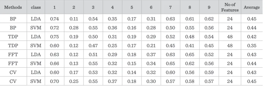
propor-tion of execupropor-tion of a given algorithm is the maximum value of the kappa coefficient from the computed time-course. The final results for the individual fea-ture extraction methods are presented in Table 1. Two classifiers, namely, the Linear Discriminant Analysis (LDA) [20] and support vector machine (SVM) [5] were utilized to evaluate the individual feature ex-traction methods.

The best results were obtained when BP and CV fea-tures were used. When utilizing band power feafea-tures with LDA classifier, the kappa value on the testing set was equivalent to 0.45, on this term of SVM it is 0.44. When using CV features with SVM classifier, the test-ing set was equivalent to 0.45 as well, on this term of LDA it is 0.43.

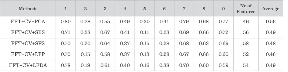
The average accuracies of the combination of meth-ods are presented in Table 2. The two methmeth-ods of feature extraction and feature reduction of PCA are combined. The best results for most subjects were achieved when using the FFT, CV and PCA in com-bination with SVM classifier. The kappa coefficient for this combination is equivalent to 0.54 when using SVM classifier and 0.48 when using the LDA classifier.

Table 1

Average accuracy of single methods

Methods class 1 2 3 4 5 6 7 8 9 _{Features Average}No of

BP LDA 0.74 0.11 0.54 0.35 0.17 0.31 0.63 0.61 0.62 24 0.45

BP SVM 0.72 0.28 0.55 0.36 0.16 0.28 0.50 0.55 0.56 24 0.44

TDP LDA 0.75 0.19 0.50 0.31 0.19 0.29 0.52 0.48 0.54 48 0.42

TDP SVM 0.60 0.12 0.47 0.25 0.17 0.21 0.45 0.41 0.45 48 0.35

FFT LDA 0.63 0.12 0.51 0.29 0.18 0.37 0.63 0.65 0.52 24 0.43

FFT SVM 0.66 0.13 0.55 0.32 0.15 0.34 0.65 0.62 0.56 24 0.44

CV LDA 0.60 0.17 0.53 0.32 0.14 0.32 0.60 0.56 0.59 24 0.43