SUPPORTING THE CHANGE IN THE DEGREE OF CONTAINMENT
IN A MULTIDIMENSIONAL MODEL
Francisco Moreno, Fernando Arango
Escuela de Sistemas, Universidad Nacional de Colombia Carrera 80 # 65 - 223, Medellín, Antioquia e-mail:[email protected], [email protected]
Iván Amón Uribe
Grupo de Investigación GIDATI, Universidad Pontificia Bolivariana Circular 1 # 70 – 01, Medellín, Antioquia
e-mail: [email protected]
Abstract. A data warehouse is usually modeled using a multidimensional view of data. A multidimensional model has dimensions composed of levels hierarchically organized according to their full containment. For example, in a geographical dimension with Department and Country levels, a department is fully contained in a country. Recently, a generalization of full containment has been proposed. It is known as the partial containment. For example, only 0.2 (20%) of a highway could be contained in a department. In this paper we adopt a multidimensional model that supports partial containment and extend this model in order to support the change of the degree (percentage) of containment, because this degree can change over time. Our extension is also incorporated into a multidimensional query language, which enables what-if analysis. In order to illustrate the expediency of our proposal, we present a case study related to car accidents.
Keywords: Multidimensional models, data warehouses, full containment, partial containment, temporality.
1. Introduction
A data warehouse [7, 9] is a database that is specially designed to support decision-making. A data warehouse is usually modeled using a multidimensio-nal view of data. Several multidimensiomultidimensio-nal models have been proposed [1, 5, 6, 8, 11, 16, 18, 20]. These models share a set of key concepts such as dimension, hierarchy, level, fact, measure, among others.
A multidimensional model has several dimensions,
e.g., the Time dimension and the Location dimension that are associated with a phenomenon of interest of an organization, known as fact, e.g., car accidents.
A dimension represents a business perspective to analyze the facts and is composed of a non-empty set of levels of aggregation [10] (Day, Month, and Year
are levels in our Time dimension; Highway, Depart-ment, and Country are levels in our Location dimen-sion, see Section 2).
On the other hand, a fact has measures, i.e., indi-cators to evaluate specific activities of an organization [13], e.g., the number of accidents and casualties, on which both calculations and reports are focused.
The levels of a dimension are hierarchically or-ganized according to the analysis needs [19]. This hierarchical organization captures the full containment
relationship between levels. For example, in our
Location dimension, a department is fully contained in a country. On the other hand, Jensen et al. [8] pro-posed a generalization of full containment, the partial containment.
The partial containment allows us to represent situations in which a dimension value is not fully con-tained in another. For example, a highway can be contained only 0.2 (20%) in a department.
However, the model of Jensen et al. [8] does not support a possible change in the degree (percentage) of containment between two dimension values. For example, at a time ti the degree of containment of a
highway in a department is 0.2, but at a time ti+1, this
well, which enables what-if analysis, a very important decision support process as stated in Balmin et al. [2].
This paper is organized as follows: in Section 2, we present a motivating example and then in Section 3, we present a multidimensional model that supports partial containment. Next, in Section 4, we introduce the extension to support the change in the degree of containment and in Section 5, we incorporate our ex-tension into a multidimensional query language, give examples, and present some basic experiments. Finally, in Section 6 we draw conclusions and outline future work.
2. A motivating example
Consider the road infrastructure of a country com-posed of highways that run through its departments (states). Figure 1 illustrates a situation where three highways (Hw1, Hw2, and Hw3) run through three
departments (Dep1, Dep2, and Dep3).
Hw1
Hw2 Hw3 Dep1
Dep2
Dep3
Figure 1. Road infrastructure of a country
The traffic authorities are interested in analyzing such things as car accidents, e.g., to identify what highways have a higher accident rate in order to im-prove their control, change its route, or take other measures to reduce accidents. In this scenario, acci-dents are the phenomena of interest, i.e., they are the facts that occur in one place and at a certain date (geo-graphical and temporal dimensions). Figure 2 presents a multidimensional model to represent this situation (the notation of Jensen et al. is used [8]) and Table 1 shows a sample data of the fact table of accidents. Note that each fact instance corresponds to the set of accidents that occurred in a highway at a particular date.
Table 1. Sample data of the fact table of accidents.
Levels Measures
Day Highway #Accidents #Casualties
…
2008-Jan-01 Hw1 2 5
2008-Jan-01 Hw2 1 2
2008-Jan-02 Hw1 3 9
2008-Jan-02 Hw2 1 2
2008-Jan-03 Hw3 1 3
2008-Jan-04 Hw2 2 4
…
2008-Jan-20 Hw2 3 3
…
Day Year
Department Country
All All
Accidents
#Accidents #Casualties Partial containment
Full containment
Month Time
dimension
Highway Location
dimension
Figure 2. Multidimensional model for the analysis of accidents
Suppose that the degree of containment of the highway Hw2 in the department Dep2 is 0.2 and in the
department Dep3 is 0.8. Consider the query: What is
the total number of accidents that have occurred in the department Dep2?
From Figure 1 it is noted that the facts associated with the highway Hw3 contribute to the total requested
since that highway is fully contained in the department Dep2; however, with regard to the facts associated
with the highway Hw2 there is not such certainty.
Nevertheless, it is possible to give an approximate answer to this query, see Table 2, if we consider the degree of containment of a highway in a department and the data are distributed proportionately.
Table 2. Calculation of the total number of accidents in the department Dep2 (a degree of containment equal to 0.2 of
the highway Hw2 in the department Dep2 is considered)
Highway
Total number of
accidents
Degree of containment
in the department
Dep2
Estimated number of accidents in
the department
Dep2
Hw1 5 0.2 5 * 0.2 = 1
Hw2 7 0.2 7 * 0.2 = 1.4
Hw3 1 1 1 * 1 = 1
Total 3.4
Suppose now that the degree of containment of the
highway Hw2 in the departments Dep2 and Dep3
changes as shown in Figure 3. The degree of containment of the highway Hw2 in both departments
Hw2
Dep2
Dep3
Dep2
Hw2 Dep3
Figure 3. Change in the partial containment: growth of the highway Hw2
Consider again the query raised and suppose that the new highway section will be available for vehicle traffic from 2008-Jan-15. Note that we must keep the evolution of changes in the degrees of containment of the highways in the departments, in order to obtain consistent results over time. Otherwise, all the facts prior to 2008-Jan-15 associated with the highway Hw2, would give the impression that they occurred
when the degree of containment of the highway Hw2
in both departments was 0.5.
Table 3 shows the results that we obtain by apply-ing the current degree of containment to all the data,
i.e., without considering the degree of containment at the time when the facts occurred (5.5 accidents).
Table 3. Calculation of the total number of accidents in the department Dep2 (current degree of containment of the
highway Hw2 in the department Dep2 is considered)
Highway
Total number of
accidents
Degree of containment
in the department
Dep2
Estimated number of accidents in
the department
Dep2
Hw1 5 0.2 5 * 0.2 = 1
Hw2 7 0.5 7 * 0.5 = 3.5
Hw3 1 1 1 * 1 = 1
Total 5.5
On the other hand, the results of Table 4 are con-sistent with regard to the degree of containment at the time when the facts occurred (4.3 accidents).
Table 4. Calculation of the total number of accidents in the department Dep2 (the degree of containment at the time
when the facts occurred is considered)
Highway
Total number of
accidents
Degree of containment
in the department
Dep2
Estimated number of accidents in
the department
Dep2
Hw1 5 0.2 5 * 0.2 = 1
Hw2 4 0.2 4 * 0.2 = 0.8
Hw2 3 0.5 3 * 0.5 = 1.5
Hw3 1 1 1 * 1 = 1
Total 4.3
In the model of Jensen et al. [8] the history of such changes is not preserved. In Section 4, we present the
corresponding extension in order to support this situation.
3. Multidimensional model with partial containment
We present next the essential concepts of the multidimensional model of Jensen [8] which supports partial containment.
3.1. Multidimensional schema
A multidimensional schema is a two-tuple S = (F,
DT), where F is a fact type and DT = {dti, i = 1,…, n}
is a set of dimension types. A dimension type dt is a four-tuple (LTdt, @, All, ↓), where LTdt = {lti, i = 1,…,
k} is a set of level types. @ is a partial order on the set
LTdt. All is the top element of the partial order and ↓
represents the bottom element of the partial order. All
represents the highest grouping level of the dimensional values and ↓ the lowest. The domain of
All is a single value: dom(All) = {all}.
Example 1. Let Accidents = {A, DT} be a multidi-mensional schema, where A is a fact type for represen-ting accidents and DT = {Time, Location}:
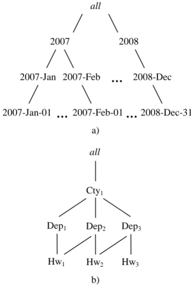
• Time = (LTTime, @, All, ↓), LTTime = {Day, Month,
Year, All}, and ↓ = Day. The corresponding partial order is shown in Figure 4 (a).
• Location = (LTLocation, @, All, ↓), LTLocation =
{Highway, Department, Country, All}, and ↓ =
Highway. The corresponding partial order is shown in Figure 4 (b).
Note that to represent a partial order, its transitive reduction is used (Hasse diagram [4]).
Figure 4. Dimension types: a) Time and b) Location
3.2. Dimension instance
Given a multidimensional schema S = (F, DT), a dimension instance d, of type dt∈DT, is a two-tuple d
= (Ld, §), where Ld = {li, i = 1,…, k} is a set of levels.
Each level l is of type lt∈LTdt, i.e., a level l is a set of
values of type lt. § is a partial order on ∪jlj (union of
Day
a) b) Month
Year All
Department Country
all the values of the levels of a dimension instance). We henceforth write Dim instead of ∪jlj.
Example 2. Let time be an instance of the dimension type Time and location an instance of the dimension type Location, see Example 1:
• time = {Ltime, §}, Ltime = {day, month, year,
all_time}, where day is of type Day, month is of type Month, year is of type Year, and all_time is of type All. day = {2007-Jan-01, 2007-Jan-02,…,
2008-Dec-31}, month = {2007-Jan, 2007-Feb,…,
2008-Dec}, year = {2007, 2008}, and all_time = {all}. The corresponding partial order is shown in Figure 5 (a).
• location = {Llocation, §}, Llocation= {highway,
depart-ment, country, all_location}, where highway is of type Highway, department is of type Department,
country is of type Country, and all_location is of type All. highway = {Hw1, Hw2, Hw3}, department
= {Dep1, Dep2, Dep3}, country = {Cty1}, and
all_location = {all}. The corresponding partial or-der is shown in Figure 5 (b).
2007-Jan-01 2007-Feb-01 2008-Dec-31 2007-Jan 2007-Feb 2008-Dec
2007 2008 all
…
…
Hw1
all
Dep1
Cty1
Hw2 Dep2
Hw3 Dep3 a)
b)
…
Figure 5. Dimension instances: a) time and b) location
3.3. Degree of containment
Given two dimension values a ∈ Dim and b ∈
Dim, and a number g ∈ [0; 1], the notation a §g b
means that a is contained in b at least in g * 100%. g
is the degree of containment of a in b. If g = 1 means that a is fully contained in b and if g = 0 means that a may be contained in b (if containment does exist, the value of the degree is unknown).
In [8] Jensen et al. present several transitivity rules to infer degrees of containment between dimension values. In the following, c∈Dim, p∈ [0; 1), and q∈
[0; 1).
i) Transitivity of full containment: if a §1b and b §1c
then a §1c,
ii) Transitivity between partial and full containment: if a §pb and b §1c then a §pc,
iii) Transitivity between full and partial containment: if a §1b and b §pc then a §0c, and
iv) Transitivity of partial containment: if a §pb and b
§qc then a §0c.
For example, the rule iii) states that if a is fully contained in b and b is contained in c in p * 100% (p < 1), then it can only be inferred that amay be contained in c (a §0c).
3.4. Fact-dimension relation
A fact-dimension relation r is defined as r ⊆f × Dim, where f is a set of facts of type F, see subsection 3.1. Each fact must be related to at least one value of each dimension. For simplicity we assume that each fact is related to only a value of each dimension and the corresponding dimension value belongs to the bottom level of the dimension.
Example 3. Consider again Example 1. Let
accidents = {Ac1, Ac2, Ac3, Ac4, Ac5} be a set of facts
of type A. Let the fact-dimension relations be:
• r1 = {(Ac1, 2008-Jan-01), (Ac2, 2008-Jan-01),
(Ac3, 2008-Jan-02), (Ac4, 2008-Jan-02), (Ac5,
2008-Jan-03)}.
• r2 = {(Ac1, Hw1), (Ac2, Hw2), (Ac3, Hw1), (Ac4,
Hw2), (Ac5, Hw3)}.
The relations r1 and r2 associate the set of facts
accidents with the values of the time dimension
instance as well as with the location dimension
instance from Example 2, respectively.
3.5. Fact characterization
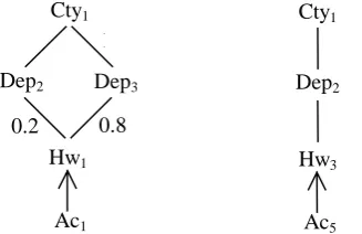
The term fact characterization is defined from a fact-dimension relation r. It is said that a fact is cha-racterized by a dimension value, if the fact is asso-ciated directly or indirectly (by transitivity in the par-tial order § of the dimension values) with such value,
i.e., a fact f1∈f is characterized by a value v1∈Dim,
written f1→v1, if: (f1, v1) ∈r or if there exists a value
v2∈Dim such that (f1, v2) ∈r and v2 § v1.
Example 4. In Figure 6: Ac1→ Hw1, Ac1 → Dep2,
Ac1 → Dep3, Ac1 → Cty1, Ac5→ Hw3, Ac5 → Dep2,
and Ac5 → Cty1.
3.6 Multidimensional object
a MO is a data cube [15], i.e., a group of cells (that contain the measures) associated with a set of dimension values. Formally, a MO is a four-tuple MO
= (S, f, D, R), where S = (F, DT) is a multidimensional schema, f is a set of facts of type F, D is a set of dimension instances each one of type dt∈DT, and R
is a set of fact-dimension relations.
Hw1 Dep2 Dep3
0.2 0.8
Ac1 Cty1
1
Hw3 Dep2
Ac5 Cty1
Figure 6. Facts Ac1 andAc5 associated with dimension
values
Example 5. Let AccidentsCube = (Accidents, acci-dents, {time, location}, {r1, r2}) be a MO, where
Accidents is the multidimensional schema of Example 1, accidents the set of facts of Example 3, {time,
location} is the set formed by the dimension instances from Example 2, and {r1, r2} is the set formed by the
fact-dimension relations from Example 3.
4. Support of the change in the degree of containment
The degree of containment between two dimension values may change over time. For example, in Figure 3 it is shown the change in the degree of containment between a) the highway Hw2 and the department Dep2
and b) the highway Hw2 and the department Dep3.
In order to support the change in the degree of containment, the following extension to the model of the previous section is proposed. Let (LTdt, @, All, ↓,
μ) be a dimension type, where μ is a temporal unit (hours, days, months, years, among others). μ defines the temporal accuracy required (granularity) for the application to record the degree of containment between the dimension values.
Consider a pair of level types (lt1, lt2) ∈LTdt. Let d
= (Ld, §) be a dimension instance, of type dt. Let the
level l1∈Ld be of type lt1and the level l2∈Ld be of
type lt2. For the pair (l1, l2) a DC (Degree of
Containment) function is defined with signature: l1 ×
l2 × dom(μ) Æ [0;1]. The DC function returns the
degree of containment at a given time of a value of l1
with regard to a value of l2.
Example 6. Let Location = (LTLocation, @, All, ↓,
μ) be a dimension type, where μ = day. Consider the
pair of level types (Highway, Department) from
Example 1. Let location = {Llocation, §} be an instance
of the dimension type Location, Llocation= {highway,
department, country, all_location}, highway is of
level type Highway and department is of level type
Department. For the pair (highway, department) a DC function is defined; some of their values are shown in Table 5 and are illustrated in Figure 7. For example, DC(Hw2, Dep3, 2008-Jan-01) = 0.8 and DC(Hw2,
Dep3, 2008-Jan-15) = 0.5.
Table 5. Sample data of the DC function for (highway,
department). hw ∈ highway, dp ∈ department, and t ∈ dom(Day)
hw dp t DC
…
Hw2 Dep2 2008-Jan-01 0.2
Hw2 Dep3 2008-Jan-01 0.8
Hw2 Dep2 2008-Jan-02 0.2
Hw2 Dep3 2008-Jan-02 0.8
…
Hw2 Dep2 2008-Jan-15 0.5
Hw2 Dep3 2008-Jan-15 0.5
…
Hw2 Dep2 Dep3
0.2 0.8
Hw2 Dep2 Dep3
0.5 0.5
a) b)
Figure 7. Degree of containment of the highway Hw2 in the
departments Dep2 and Dep3: a) between 2008-Jan-01
and 2008-Jan-14 and b) from 2008-Jan-15
For calculating the degree of containment between two dimension values that are not adjacent in the hierarchy, the rules of transitivity from the subsection 3.3 are applied.
Example 7. Consider Figure 1 and suppose that the DC(Hw1, Dep1, 2008-Jan-31) = 0.8, see Figure
8(a). Suppose that from 2008-Feb-01, the section of the highway Hw1 in the department Dep2 is
elimi-nated, thus DC(Hw1, Dep1, 2008-Feb-01) = 1, see
Figure 8(b). Therefore, by applying the transitivity rules, it is obtained that DC(Hw1, Cty1, 2008-Jan-31)
= 0.8 and DC(Hw1, Cty1, 2008-Feb-01) = 1.
Hw1 Dep1
0.8 Cty1
a) b) Hw1
Dep1
1 Cty1
Figure 8. Degree of containment of the highway Hw1 in the
5. Integration into a multidimensional language
This section illustrates how our proposed exten-sion can be incorporated into a multidimenexten-sional que-ry language. We present also some basic experiments related to accidents in Mexican highways.
5.1. Language
Although MDX (Multidimensional Expressions) [21] is a language which in recent years has become a
de facto standard to query multidimensional data, we use the language proposed by Datta and Thomas [3], because of its similarity to the relational algebra. We use the operators of restriction (σ) and aggregation
(α). We give next a brief description of these
operators. For details, refer to Datta and Thomas [3]. i) σ: allows us to specify values for dimensions.
Notation: σP(Cube1) = Cube2, where P is a
predicate and
ii) α: applies aggregate functions to measures with one or more levels of a dimension specified as grouping attributes. Notation: α [AL, GDL](Cube1) =
Cube2. AL is a list of elements gi(mi) where gi is an
aggregate function applied to measure mi and GDL
is a set of grouping dimensions levels.
For all the queries, the AccidentsCube cube from the Example 5 is used.
Query 1. What is the total number of accidents that have occurred in the department Dep2?
α[SUM(#Accidents * DC(highway, 'Dep2', day))](AccidentsCube)
That is, all the facts from the AccidentsCube cube are selected. Then for each fact, the degree of containment of the corresponding highway in the
department Dep2 is found, and this value is then
multiplied by the number of accidents. Next, the total requested is obtained using the aggregate funtion SUM. The same query formulated in a SQL-like way is:
SELECT SUM(#Accidents * DC(highway, 'Dep2', day))
FROM AccidentsCube
Note that to calculate the degree of containment the date (day) associated with the fact is used, i.e., the degree of containment at the time when the facts occurred is used. However, it is possible to formulate hypothetical queries in order to analyze past behaviors and make predictions, as exemplified in the following queries.
Query 2. What would the total number of acci-dents have been in the department Dep2 if the existing
degree of containment in the highways in such depart-ment in 2007-Jan-01 was considered?
α[SUM(#Accidents * DC(highway, 'Dep2', '2007-Jan-01'))]((AccidentsCube))
In this query, all the facts from the AccidentsCube
cube are considered, e.g., facts from 2007 and from 2008, but the degree of containment corresponding to 2007-Jan-01 is used.
Query 3. What would the total number of accidents have been in the department Dep2 in 2007
given the current degree of containment of highways in that department? The current date is represented by
now.
α[SUM(#Accidents * DC(highway, 'Dep2', now))](σday > '2007-Jan-01' AND day <
'2007-Dec-31'(AccidentsCube))
In this query, only the facts from the Accidents-Cube cube from 2007 are selected, but the degree of containment corresponding to the current date is used.
5.2. Experiments
In order to make some basic experiments we im-plemented our multidimensional model for the analy-sis of accidents in a relational way using Oracle. We implemented the DC function using a many-to-many relationship between highway and department and a stand-alone Oracle function that was invoked from SQL queries.
Baja Calif.
Sonora
Mexico
Morelos
Oaxaca Veracruz
Sonora Baja
Calif.
Mexico
Morelos
Oaxaca Veracruz
a) b)
c) d)
e) f)
M-002D M-002D
M-115
M-185 M-185
M-115
Figure 9. Configuration of highways: a) highway M-002D in 2002, b) highway M-002D in 2005, c) highway M-115 in
2002, d) highway M-115 in 2005, e) highway M-185 in 2002, and f) highway M-185 in 2005
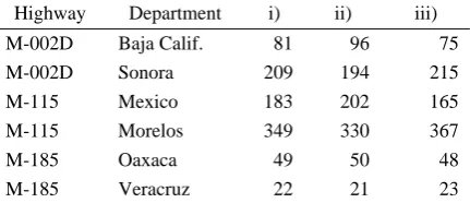
of accidents in these highways and in Table 7 we indi-cate the degree of containment of each highway in each department. Finally, in Table 8 we present the corresponding calculations of the total number of ac-cidents in each department:
i) applying the corresponding degree of containment at the time when the accidents occurred,
ii) applying to all the accidents, the degree of contain-ment of the highways in 2002, and
iii) applying to all the accidents, the degree of contain-ment of the highways in 2005.
For example, the calculations for highway M-002D and department Baja California in Table 8 are made as follows. Column i) 84 * 0.33 + 206 * 0.26 = 81, column ii) (84 + 206) * 0.33 = 96, and column iii) (84 + 206) * 0.26 = 75.
Table 6. Number of accidents in 2002 and 2005
Highway Year #Accidents
M-002D 2002 84
M-002D 2005 206
M-115 2002 263
M-115 2005 269
M-185 2002 26
M-185 2005 45
Table 7. Degree of containment of each highway in each department in 2002 and 2005
Highway Year Department Length (km)
Degree of containment
M-002D 2002 Baja Calif. 46.46 0.33
M-002D 2002 Sonora 92.94 0.67
M-002D 2005 Baja Calif. 46.46 0.26
M-002D 2005 Sonora 134.84 0.74
M-115 2002 Mexico 50.21 0.38
M-115 2002 Morelos 80.69 0.62
M-115 2005 Mexico 50.21 0.31
M-115 2005 Morelos 110.24 0.69
M-185 2002 Oaxaca 168.49 0.71
M-185 2002 Veracruz 68.11 0.29
M-185 2005 Oaxaca 168.49 0.67
M-185 2005 Veracruz 84.21 0.33
Table 8. Calculations of the total number of accidents: i) using the degree of containment at the time when the accidents occurred, ii) using the degree of containment in 2002, and iii) using the degree of containment in 2005.
Highway Department i) ii) iii)
M-002D Baja Calif. 81 96 75
M-002D Sonora 209 194 215
M-115 Mexico 183 202 165
M-115 Morelos 349 330 367
M-185 Oaxaca 49 50 48
M-185 Veracruz 22 21 23
6. Conclusions and future work
In this work we adopted a multidimensional model that supports partial containment. This model was ex-tended to allow for the possible change in the degree of containment between dimension values.
The extension was also incorporated into a multi-dimensional query language. This allows queries that are consistent with time and furthermore, allows the formulation of hypothetical queries (what if?, what would have happened if?), which can help decision makers.
As future work, we plan to incorporate our propo-sal into a platform such as Pentaho [17] or Microsoft Analysis Server [14]. However, since these platforms are directed to the management of multidimensional models that support full containment, the introduction of our extension poses interesting challenges.
On the other hand, from the point of view of language, both platforms support MDX. However, since MDX is also directed to the management of full containment, the incorporation of our proposal into this language brings challenges as well.
Finally, more extensive experiments and analysis are needed in order to try to identify possible beha-viors. It would be interesting to analyze other domains where partial containment arises, e.g., facts as crimes and fish catches, associated with regions that are located among several countries or departments.
Acknowledgments
This paper is part of the first author’s Ph.D. work, sponsored by Colciencias, in Ingeniería - Sistemas, Universidad Nacional de Colombia, Sede Medellín.
References
[1] R. Agrawal, A. Gupta, S. Sarawagi. Modeling Multidimensional Databases. 13th International Confe-rence on Data Engineering (ICDE’97), Birmingham,
UK. 1997, 232-243.
[2] A. Balmin, T. Papadimitriou, Y. Papakonstantinou. Hypothetical Queries in an OLAP Environment. 26th
International Conference on Very Large Data Bases (VLDB), Cairo, Egypt, 2000, 220-231.
[3] A. Datta, H.Thomas. The Cube Data Model: a Con-ceptual Model and Algebra for On-line Analytical Processing in Data Warehouses. Decision Support Systems, Vol.27 (3), 1999, 289-301.
[4] R. Freese. Automated Lattice Drawing. 2nd Inter-national Conference on Formal Concept Analysis
(ICFCA'04), Sydney, Australia, 2004, 112-127. [5] M. Golfarelli, S.Rizzi. A Methodological Framework
for Data Warehouse Design. 1st ACM International Workshop on Data Warehousing and OLAP
(DOLAP’98), Washington D.C. USA, 1998, 3-9. [6] M. Gyssens, L. Lakshmanan. A Foundation for
[7] W. Inmon. Building the Data Warehouse. Wiley, New York, USA. 4th ed. 2005, 576.
[8] C. Jensen, A. Kligys, T. Pedersen, I.Timko. Multi-dimensional Data Modeling for Location-based Services. 10th ACM International Symposium on
Ad-vances in Geographic Information Systems (GIS
2002), McLean, USA, 2002, 55-61.
[9] R. Kimball, M. Ross, W. Thornthwaite, J. Mundy, B. Becker. The Data Warehouse Lifecycle Toolkit.
Wiley, New York, USA, 2nd ed. 2008, 672.
[10] N. Kumar, A. Gangopadhyay, S. Bapna, G. Kara-batis, Z.Chen. Measuring Interestingness of Discove-red Skewed Patterns in Data Cubes. Decision Support Systems, Vol. 46, (1), 2008, 429-439.
[11] W. Lehner, J. Albrecht, H. Wedekind. Normal Forms for Multidimensional Databases. 10th Interna-tional Conference on Scientific and Statistical Data-base Management (SSDBM’98), Capri, Italy, 1998, 63-72.
[12] IMT: Instituto Mexicano del Transporte. Anuario Estadístico de Accidentes en Carreteras Federales
1997 – 2006. http://www.imt.mx/Espanol /Publicacio-nes/. Date of access July 2009.
[13] E. Malinowski, E. Zimányi. Advanced Data Ware-house Design: From Conventional to Spatial and Temporal Applications. Springer, New York, USA, 2008, 435.
[14] Microsoft. Microsoft SQL Server 2008.
http://www.microsoft.com/sqlserver/2008/en/us. Date of access June 2009.
[15] OLAP Council. The OLAP Glossary.
http://www.olapcouncil.org/research/resrchly.htm. Date of access May 2009.
[16] T.B. Pedersen, C.S. Jensen, C.E.Dyreson. A Foun-dation for Capturing and Querying Complex Multidi-mensional Data. Information Systems, Vol.26(5), 2001, 383-423.
[17] Pentaho. Pentaho BI Suite Enterprise Edition. http://www.pentaho.com. Date of access June 2009. [18] I. Timko, C. Dyreson, T. Pedersen. Probabilistic
Data Modeling and Querying for Location-based Data Warehouses. 17th International Conference on Scien-tific and Statistical Database Management (SSDBM
2005), Santa Barbara, USA, 2005, 273-282.
[19] R. Torlone. Conceptual Multidimensional Models. In: M. Rafanelli (Ed.), Multidimensional Databases: Problems and Solutions, Idea Group Publishing, Pennsylvania, USA, 2003, 69-90.
[20] P.Vassiliadis. Modeling Multidimensional Databases, Cubes and Cube Operations. 10th International Confe-rence on Scientific and Statistical Database Manage-ment (SSDBM’98), Capri, Italy, 1998, 53-62.
[21] M. Whitehorn, R. Zare, M.Pasumansky. Fast Track to MDX. Springer, New York, USA, 2nd. ed. 2006, 310.