SOLUTION AND ANALYSIS OF CFD APPLICATIONS BY USING
GRID INFRASTRUCTURE
Arnas Ka
č
eniauskas
Laboratory of Parallel Computing, Vilnius Gediminas Technical University Saulėtekio St. 11, Vilnius, LT-10223, Lithuania
e-mail: [email protected]
Abstract. The paper describes solution and analysis of complex computational fluid dynamics (CFD) applications by using grid infrastructure. Powerful and flexible computing environment including computing resources, data sto-rage, simulation software, visualization e-service and graphical job monitoring tool is developed and employed for solution of CFD problems. Efficiency of parallel computations is evaluated by performing a benchmark based on con-vective pollution transport. Challenging dam break flow simulation including highly non-linear breaking waves requires all advanced features of modern BalticGrid infrastructure. The numerical results are validated by quantitative comparison with the experimental measurements.
1. Introduction
Computational fluid dynamics (CFD) plays an im-portant role in the design of modern industrial compo-nents [2]. Many industrial applications described by the Navier-Stokes equations are solved by CFD codes [27]. Numerous examples include actual problems such as oil filters, pollution transport, sluice gates and tank sloshing. Various computational methods are de-veloped for discretizing the governing equations and spatial domains. The finite element method (FEM) [30] has the capability of accepting complex geomet-ries in an integrated fashion, making it particularly interesting to the designers of complex mechanisms. However, it has always been the problem of the FEM that larger computational times have been associated with it. Grid computing [6] is thus perceived as a promising avenue for future advances in this applied area of science.
European Grid Infrastructure [4] can provide re-sources for solving large industrial CFD problems. Grid computing represents one of the most promising advancements for modern computational science. With the power of grid, scientists are able to perform simulations at previously impossible and unexplored problem scales. Grid development efforts push para-digms of remote HPC resource usage [7]. Scientists who used to login to the supercomputer of their choice to submit computing jobs are now presented with an interface that can assign their computational workload to a pool of resources anywhere in their Virtual
Organization (VO). However, this leads to very comp-licated environments handling complex simulation on remote heterogeneous architectures [21]. The design of distributed parallel algorithms and the software deployment in grid [5] presents a new challenge to computational scientists. Recent progress resulted in the dramatic increase of computational capacity, which approached the petaflop level.
BalticGrid [3] infrastructure is built on gLite middle-ware [9], developed within EGEE. Only part of Glo-bus functionality can be accessed in the considered grid environment, therefore, most of available visuali-zation software, web portals and graphical user inter-faces cannot be directly applied.
The paper presents powerful and universal compu-ting environment employed for solution and analysis of CFD applications. Software integration and deploy-ment issues are covered in details. Grid visualization e-service VizLitG is developed for interactive visua-lization of remote data files located in grid storage elements. The performance analysis reveals how effi-ciently CFD applications can be solved on gLite based grid infrastructure.
2. Description of investigated CFD problems
Several actual CFD applications like oil filters, sediment transport, oil reservoirs and dam break flows have been investigated on BalticGrid infrastructure. In this section, two pilot CFD applications are described. A rotating cone problem originated from the investiga-tion of convective polluinvestiga-tion transport can be conside-red as a test problem for stabilisation methods and parallel algorithms. A dam break problem includes complex breaking wave phenomena that require advanced modelling techniques, impressive compu-ting resources and flexible simulation software.
Figure 1. Rotating cone after 2π period of time
The rotating cone problem (Figure1) is widely used to illustrate the effectiveness of algorithms in case of convection dominated flows. The 2D square solution domain [-0.5; 0.5]x[-0.5; 0.5] is discretized by structured finite element meshes. The concentration cone of radius 0.15 is positioned at (-0.25; 0.0). In the centre of the cone, the concentration maximum of 1.0 decreases to zero as sinusoidal curve. The velocity field u = -y, v = x corresponds to a rotational flow with a nature of a solid body. The problem is numerically difficult to solve not only because of the pure ad-vection but also because of the numerical diffusion
attributed to the Cartesian grid discretizing the rota-tional flow field.
The dam break problem including the breaking wave phenomena has been the subject of extensive research for a long time [18, 22, 24]. However, the universal, accurate and efficient numerical technique for breaking wave simulation attracts big attention of research community and software developers. Measu-rements of the exact interface shape are not available, but some secondary data such as reduction of the water column height can be employed for quantitative comparison of the results [22].
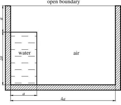
a
4a a
2
a
open boundary
air water
Figure 2. Geometry of the dam break problem
The geometry of the solution domain is shown in Figure2. The dimensions of the reservoir and the water column correspond to those used in the experi-ment carried out by Koshizuka et. al. [18]. The reser-voir is made of glass, with a base length of 0.584 m. The water column, with a base length of 0.146m and the height of 0.292 m (a = 0.146 m), was initially supported on the right by a vertical plate drawn up rapidly at time t = 0.0 s. The water falls by gravity (g = 9.81 m/s2), acting vertically downwards. The density of water is ρA = 1000 kg/m3, while the dynamic
vis-cosity coefficient is μA = 0.01 kg/(m⋅s). The density
of air is taken to be ρB = 1 kg/m3, and the dynamic
viscosity coefficient is μB = 0.0001 kg/(m⋅s).
3. Governing equations
The laminar and Newtonian flow of viscous and incompressible fluids is considered. It is governed by the Navier-Stokes equations (the Eulerian reference frame)
ij
i i
j i
j j
u u
u F
t x x
σ ρ⎛⎜⎜∂ + ∂ ⎞⎟⎟=ρ +∂
∂ ∂ ∂
⎝ ⎠ , (1)
0
= ∂ ∂
i i x u
where ui are the velocity components; ρ is the density;
Fi are the gravity force components and σij is stress
tensor
j i
ij ij
j i
u u p
x x
σ = − δ +μ⎛⎜⎜∂ +∂ ⎞⎟⎟
∂ ∂
⎝ ⎠, (3)
where μ is dynamic viscosity coefficient; p is pressure and δij is Kronecker delta.
The pseudo-concentration method [28] is develo-ped for moving interface flows using the Eulerian approach and the interface capturing idea. The pseu-do-concentration function ϕ serves as a marker, iden-tifying fluids A and B with densities ρA and ρB and
viscosities μAand μB. In this context, the density and
viscosity are defined as:
B
A ϕ ρ
ϕρ
ρ = +(1− ) , (4)
B
A ϕ μ
ϕμ
μ= +(1− ) , (5)
while ϕ = 1 for fluid A and ϕ = 0 for fluid B.
The evolution of the moving interface as that of pollution concentration is governed by a time dependent convection equation
0
= ∂
∂ + ∂ ∂
j j x u t
ϕ ϕ
. (6)
The initial conditions defined on the entire solution domain should be prescribed for the equation (6). In case of equations (1)-(3), the slip boundary conditions are prescribed on rigid walls while the zero stress boundary conditions are prescribed on the upper open boundary. The detailed discussion on stress dependent boundary conditions and their implementation can be found in the work [16].
The space-time Galerkin least squares finite element method [23] is applied as a general-purpose computational approach to solve the partial differen-tial equations (1)−(6). The detailed description of va-riational formulation and stabilisation parameters can be found in the work [17].
4. Software deployment on grid infrastructure
The discussed applications have been solved by the code FEMTOOL [17], designed for coupled prob-lems of CFD. FEMTOOL allows implementation of any partial differential equation with minor expenses. Time dependent problems are solved using space-time finite elements. The order of shape functions is deter-mined by input and is limited neither in space nor in time. A given transient problem can be solved in seve-ral implicit time steps from one time level to the other or in one single implicit step for all time levels. Space-time finite element integration in Space-time and the high order shape functions generated automatically make FEMTOOL to be applicable to complex CFD applica-tions of interest.
Several times FEMTOOL software was deployed on gLite based grid. The gLite Workload Management System (WMS) natively supports the submission of MPI jobs, which are jobs composed of a number of processes running on different Working Nodes (WN) in the same Computing Element (CE). However, this support is still experimental, therefore, running MPI applications on the gLite grid requires significant hand-tuning for each site. The first FEMTOOL de-ployment relied on shell scripts consisting of approxi-mately 100 lines. Only experienced system administ-rator can prepare such scripts for new MPI applica-tions. Recent efforts made in Interactive European Grid project slightly improved the situation [15].
The latest FEMTOOL gridification is based on the compilers g95 and gcc as well as on the OpenMPI implementation. FEMTOOL version 3.0 has been de-ployed in BalticGrid-II testbed by using SGM (Soft-ware Grid Manager) system. All soft(Soft-ware packages are installed in the predefined location, which is specified by content of $VO_BGTUT_SW_DIR vari-able. After successful installation, the SGM marks the site in global grid information system as capable of running FEMTOOL application. By use of the flag
VO-balticgrid-A-ENG-FEMTOOL-3.0, called "a tag"
the ordinary FEMTOOL users may indicate which sites they want to use.
Solution of large and complex CFD applications on heterogeneous grid infrastructure requires graphical user interface that hides the complexity of the grid middleware from the ordinary user and makes access to the grid resources easy and transparent. Migrating Desktop Platform [20] developed at the Poznan Super-computing and Networking Centre has been applied to run CFD applications on BalticGrid infrastructure. The Migrating Desktop Platform is a powerful and flexible user interface to grid resources that gives a transparent user work environment and easy access to resources and network file systems independently of the system version and hardware. It allows the user to run applications, manage data files, and store personal settings independently of the location or the terminal type. User can perform basic operations on files (downloading, uploading, transferring or removing, etc.) stored on data management systems like gLite SEs and GridFTP servers.
the metadata file of FEMTOOL, prepares the file de-fining the job, creates shell script file specifying exe-cutable with arguments and submits job to grid. Wizards of Migrating Desktop Platform handle the whole job’s life-cycle from job defining and submis-sion to job state monitoring and visualization of job results by provided software. Finally, computed results are transferred to the most suitable Storage Element.
Figure 3. FEMTOOL plug-in of Migrating Desktop
5. Visualization of remote result files
The obtained results have been processed by grid visualization e-service VizLitG designed for con-venient access and interactive visualization of remote results located in Storage Elements. VizLitG (Figu-re 4) is developed and maintained in the Laboratory of Parallel Computing of Vilnius Gediminas Technical University.
Figure 4. Connection dialog of grid e-service VizLitG
The client-server architecture of the grid visualiza-tion service is based on widely recognized web stan-dards. VizLitG has flexible environment and remote instrumentation of e-service provided by Java and GlassFish application server [8]. The visualization engine of the VizLitG is based on VTK toolkit [26]. VTK modules are enwrapped by Java programming language and build the service running on the server. The visualization server runs on the special User Interface named UIG (User Interface for Graphics). User authentification and full data transfer from SE is
performed by gLite means. Moreover, remote instru-mentation of e-service provides for users flexible access of remote data files located in grid. Transfer of interactively selected parts of datasets located in experimental SE instead of the whole data files can save significant amount of visualization time.
The developed GUI allows automatic data mana-gement and interactive dataset selection. In order to process HDF5 [13] files automatically, datasets are stored in predefined structure allowing the software to interpret the structure and contents of a file without any outside information. HDF5 groups and datasets are automatically processed considering values of HDF5 attributes. Several API’s for writing data files in predefined HDF5 format are provided for VizLitG users. C and FORTRAN90 programming languages are considered as well as C++. Time dependent and time independent data are processed differently. Data-sets that do not change in time are located in the group Common. Datasets varying in time are grouped and stored according to time step number. GUI separates geometry and topology from attributes like scalars or vectors in order to emphasize their different nature (Figure 5).
Figure 5. The data window for interactive dataset selection
A visualization network is assembled from VTK objects by using GUI. The resulting pipelines are de-scribed by XML language [29]. Valid XML documents are automatically generated on a client and transferred to the server by JAX-WS (Java API for XML Web Services) Runtime. Tabular design of GUI fields simp-ly illustrates the dataflow. Multiple VTK renderers can work in one render window. VizLitG allows grouping of complex visualizations in several viewports. The user can assign considered mappers to different view-ports.
(Figure 6) provide for remote users of the e-service full interactivity.
Figure 6. Interactive widget applied to plot stream lines
6. Numerical results and discussions
Computations have been performed on the diffe-rent sites of BalticGrid infrastructure [3]. These sites provide for BalticGrid users over 5300 CPU and 120 TB of data storages. Some of the employed Com-puting Elements belong to Lithuanian NGI (National Grid Initiative) tightly incorporated into European Grid Infrastructure.
The parallel performance of computations has been evaluated by measuring the speed-up Sp
p p t
t
S = 1
, (7)
where t1 is the program execution time for a single
processor; tp is the wall clock time for a given job to
execute on p processors. Parallel speed-up has been measured by fixing the number of particles and increasing the number of the processors used.
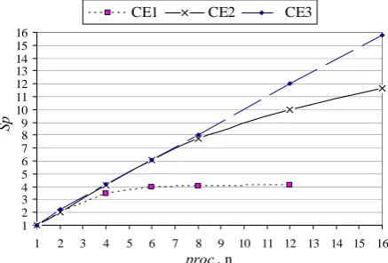
1 2 3 4 5 6 7 8 9 10 11 12 13 14 15 16
1 2 3 4 5 6 7 8 9 10 11 12 13 14 15 16
proc, n
Sp
CE1 CE2 CE3
Figure 7. Spead-up measured on different BalticGrid CEs
The considered benchmark is based on numerical solution of the rotating cone problem discretized by 160000 finite elements. The results of speed-up ana-lysis obtained on three CEs are presented in Figure 7. The speed-up (7) as a function of the number of pro-cessors is plotted. Advantages obtained by parallelism
on the site CE1 diminish rapidly as the number of pro-cessors exceeds some threshold value. This behaviour is explained by the fact that the parallel speed-up is largely determined by the ratio of local computations over inter-processor communication. As the number of processors increases, for a fixed problem size, the communication cost will eventually become dominant over the local computation cost after a certain stage. It is evident that the discussed threshold value for site CE1 is unacceptably small. The obtained results can be explained by the fact that the site CE1 is collected from the old hardware including slow 100Mbit/s net-work.
Speed-up measured on other sites CE2 and CE3 is significantly higher. When the number of processors is small, the measured speed-up is close to linear on both sites. The reduction of the efficiency owing to com-munication overhead is obtained for a larger number of processors on CE2. Nearly ideal speed-up is obser-ved on CE3 site for the considered number of pro-cessors, which is caused by perfectly balanced ratio of communications to computations.
The dam break problem is also investigated by performing numerical experiments on sustainable BalticGrid infrastructure. The computations are performed by using the structured finite element meshes of different resolution − 120×90 and 240×180. The investigated time interval is t = [0.0; 1.0]s. The size of the time step is Δt = 0.001667 for the 120×90 finite element mesh. The number of time steps is equal to 600. The size of the time step for the 240×180 finite element mesh is Δt = 0.000667. The number of the time steps used is equal to 1500. The large number of numerical parameters governing the sharpness of the front and mass conservation should be investigated in order to obtain accurate numerical solution. Available grid infrastructure is well suited for required para-metric computations.
Gravity causes the water column on the left of the reservoir to seek the lowest possible level of potential energy. Thus, the column will collapse and eventually come to rest. The initial stages of the flow are domina-ted by inertia forces. On such a large scale, the effect of surface tension forces is insignificant. The comp-lexity of velocity fields, occurring at different stages of breaking wave phenomena, can be easily captured using simple structured meshes.
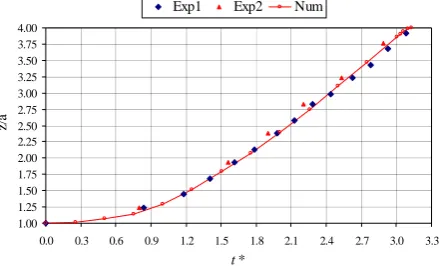
1.00 1.25 1.50 1.75 2.00 2.25 2.50 2.75 3.00 3.25 3.50 3.75 4.00
0.0 0.3 0.6 0.9 1.2 1.5 1.8 2.1 2.4 2.7 3.0 3.3
t*
z/
a
Exp1 Exp2 Num
Figure 8. Quantitative comparison of the numerical results and experimental measurements
Figure 9 shows the screenshot of grid visualization e-service VizLitG illustrating the breaking wave phenomenon often occurring in later stages of the dam break problem. Computed velocity field is represented by glyphs. Moving interface is captured by the iso-countour. Grey colours illustrate the pressure field while the chart plot shows variation of the pressure at the bottom. When t=0.83s, the backward moving wave folds over twice and small amounts of air are trapped. However, in experiments, this air is present in the form of small bubbles. The developed methodology has been derived for sharp interfaces, therefore, the mesh needs significant refinement to a resolution smaller than the bubble size.
Figure 9. Visualization of breaking wave phenomena
6. Conclusions
In this paper, analysis of complex CFD problems by using grid infrastructure has been described. Deve-lopment and application issues of modern computing environment have been discovered emphasizing soft-ware deployment on grid, automatic job submission and visualization of remote result files. Performance tests based on parallel solution of rotating cone prob-lem revealed that grid sites for efficient computations should be considered carefully evaluating potential abilities of employed hardware. The implemented do-main decomposition strategy is well designed for pa-rallel solution of convective transport problems. Challenging dam break flow simulation including highly non-linear breaking waves has required all advanced features of modern BalticGrid infrastructure. The numerical results have been validated by quantita-tive comparison with the experimental measurements. The computed position of the leading edge of the col-lapsing water column has been in good agreement with the experimental data. Performed investigation proves that the developed BalticGrid infrastructure provides powerful and flexible computing environ-ment for fast and efficient solution of challenging CFD applications.
Acknowledgement
The work described in this paper is supported by the European Union through the FP7- INFRA-2007-1.2.3: e-Science Grid infrastructures contract No 223807, project "Baltic Grid Second Phase (Baltic-Grid-II)".
References
[1] A.A. Ahmed, M.S.A. Latiff, K.A. Bakar, Z.A. Ra-jion. Visualization Pipeline for Medical Datasets on Grid Computing Environment. Proc. of 5th Int. Conf. on Computational Science and Applications, IEEE Computer Society Press, 2007, 567–575.
[2] A.J. Baker. Finite Element Computational Fluid Me-chanics. McGraw-Hill, 1983.
[3] BalticGrid:http://www.balticgrid.eu/ (Accessed June 2010).
[4] EGI: http://web.eu-egi.eu/ (Accessed June 2010).
[5] L. Field, E. Laure, M.W. Schulz. Grid deployment experiences: grid interoperation. J. Grid Computing, 2009, Vol. 7(3), 287−296.
[6] I. Foster, C. Kesselman. Grid: Blueprint for a new computing infrastructure (1st ed.). San Francisco,
[7] W. Gentzsch. Grid and cloud portals for design, simu-lation and collaboration. In Parallel, distributed and
grid Computing for engineering (Eds. Topping, B.H.V., Ivanyj, P.), Saxe-Coburg Publications, 2009, 83−116.
[8] GlassFish: https://glassfish.dev.java.net/ (Accessed
April 2010).
[9] gLite: http://glite.web.cern.ch/glite/ (Accessed June 2010).
[10] Globus: http://www.globus.org/ (Accessed June 2010).
[11] GVid: http://www.gup.jku.at/gvid/ (Accessed July 2010).
[12] C.D. Hansen, C.R. Johnson. The Visualization Handbook. Elsevier, 2005.
[13] HDF5:http://hdf.ncsa.uiuc.edu/products/hdf5/ ( Acces-sed July 2010).
[14] G. Humphreys, M. Houston, R. Ng, R. Frank, S. Ahern, P.D. Kirchner, J.T. Klosowski. Chromium: A Stream Processing Framework for Interactive Ren-dering on Clusters. ACM Transactions on Graphics, 2002, Vol. 21(3), 693–702.
[15] int.eu.grid: http://www.interactive-grid.eu/ (Accessed
April 2010).
[16] A. Kačeniauskas, R. Kutas. Implementation of stress dependent boundary conditions in FEM code for coupled problems. Information Technology and
Cont-rol, 2008, Vol. 37(1), 69–74.
[17] A. Kačeniauskas, P. Rutschmann. Parallel FEM software for CFD problems. Informatica, 2004, Vol. 15(3), 363−378.
[18] S. Koshizuka, H. Tamako, Y. Oka. A particle me-thod for incompressible viscous flow with fluid frag-mentation. Computational Fluid Dynamics, 1995, Vol. 4(1), 29-46.
[19] D. Kranzlmuller, G. Kurka, P. Heinzlreiter, J. Vol-kert. Optimizations in the Grid Visualization Kernel.
Proc. of the Workshop on Parallel and Distributed Computing in Image Processing, Video Processing and Multimedia, IPDPS 2002, Ft. Lauderdale,
Flo-rida, 2002.
[20] M. Kupczyk, R. Lichwała, N. Meyer, B. Palak, M. Płóciennik, P. Wolniewicz. “Applications on demand” as the exploitation of the Migrating Desktop.
Future Generation Computer Systems, Vol. 21(1), 2005, 37−44.
[21] M. Li, M. Baker. The Grid: Core Technologies.
Wiley, 2005.
[22] J.C. Martin, W.J. Moyce. An experimental study of the collapse of liquid columns on a rigid horizontal plane. Philosophical Transactions of the Royal Society
of London, 1952, Vol. A244, 312−324.
[23] A. Masud, T.J.R. Hughes. A Space – Time Galer-kin/Least – Squares Finite Element Formulation of The Navier-Stokes Equations for Moving Domain Problems. Computer Methods in Applied Mechanics
and Engineering, 1997, Vol. 146(1−2), 91−126.
[24] M. Quecedo, M. Pastor, M.I. Herreros, J.A. Fer-nández Merodo, Q. Zhang. Comparison of two ma-thematical models for solving the dam break problem using the FEM method. Computer Methods in Applied
Mechanics and Engineering, 2005, Vol. 194(36-38), 3984-4005.
[25] RealityGrid: http://www.realitygrid.org/ (Accessed June 2010).
[26] W. Schroeder, K. Martin, B. Lorensen. Visualiza-tion Toolkit: An Object-Oriented Approach to 3D Gra-phics, 4th Edition. Kitware. Inc., 2006.
[27] T.E. Tezduyar. Finite Elements in Fluids: Special Methods and Enhanced Solution Techniques.
Compu-ters & Fluids,2007, Vol. 36(2), 207−223.
[28] E. Thompson. Use of Pseudo-Concentrations to Fol-low Creeping Viscous FFol-lows During Transient Analysis. International Journal for Numerical
Me-thods in Fluids, 1986, Vol. 6(10), 749−761.
[29] XML: http://www.w3.org/XML/ (Accessed June 2010).
[30] O.C. Zienkiewicz, R.L. Taylor. The Finite Element Method. Vol. 1−3, the fifth edition, London,
Butter-worth Heinemann, 2000.