OPTIMIZATION OF THE GYROAVERAGE OPERATOR BASED ON HERMITE
INTERPOLATION
Fabien Rozar
1 3, Christophe Steiner
2, Guillaume Latu
3, Michel
Mehrenberger
2, Virginie Grandgirard
3, Julien Bigot
1, Thomas
Cartier-Michaud
3and Jean Roman
4Abstract. Gyrokinetic modeling is appropriate for describing Tokamak plasma turbulence, and the gyroaverage operator is a cornerstone of this approach. In a gyrokinetic code, the gyroaveraging scheme needs to be accurate enough to avoid spoiling the data but also requires a low computation cost because it is applied often on the main unknown, the 5Dguiding-center distribution function, and on the 3Delectric potentials. In the present paper, we improve a gyroaverage scheme based on Hermite interpolation used in theGyselacode. This initial implementation represents a too large fraction of the total execution time. The gyroaverage operator has been reformulated and is now expressed as a matrix-vector product and a cache-friendly algorithm has been setup. Different techniques have been investigated to quicken the computations by more than a factor two. Description of the algorithms is given, together with an analysis of the achieved performance.
1.
Introduction
Gyrokinetic modeling is appropriate for describing Tokamak plasma turbulence and the gyroaverage operator is a cornerstone of this approach. This is the model used byGysela, a simulation code which is used to study the turbulence development in plasma fusion. The gyroaverage operator J transforms the so-called guiding-center distribution into the actual particle distribution. It enables to take into account effects relative to the finite Larmor radius, which is the radius of gyration of the gyro-center (motion which is faster than the turbulence we are looking at). In the present paper, we improve the gyroaverage scheme based on interpolation of the Gysela code to speedup calculations. For the current gyroaverage operator, the Larmor radius ρ is assumed to be independent in space. This code considers a computational domain in five dimensions (3D in space describing a torus geometry, 2D in velocity) [6, 7]. Time evolution of the system consists in solving Vlasov equation non-linearly coupled to a Poisson equation (electrostatic approximation, quasi-neutrality is assumed). Routinely, physicists perform large Gysela simulations using from 1k to 16k cores on supercomputers. This work aims at improving the gyroaverage method based on Hermite interpolation which is too slow to be used in production for the moment. In achieving this optimization, we will allow the physicists to access to more accurate simulations and then to better understand the physical processes that arise in the simulations at finest scales.
1 Maison de la Simulation, USR 3441, CEA / CNRS / Inria / Univ. Paris-Sud / Univ. Versailles, 91191 Gif-sur-Yvette, FRANCE
2 IRMA, Universit´e de Strasbourg, France 3 CEA, IRFM, F-13108 Saint-Paul-lez-Durance 4 Inria, Bordeaux INP, CNRS, FR-33405 Talence
c
EDP Sciences, SMAI 2016
The use of the Fourier transform reduces the gyroaveraging operation by a multiplication in the Fourier space by the Bessel function. Good approximations of the Bessel function have been proposed such as the widely used
Pad´e expansion. The Pad´e approximation enables to recover a good approximation for small radii (see Fig. 5) [3]. However, for a larger Larmor radius and ordinary wave-numbers, the Pad´e approximation truncates the oscillations of the Bessel function, over-damps the small scales, and then introduces bias in the simulation data. Also the use of Fourier transform is not applicable in general geometry as we would like [3]; therefore it can not be employed in realistic tokamak equilibrium. These two limitations are overcome using an interpolation technique on the gyro-circles already introduced in [11] and which is the basis of our study.
In a gyrokinetic code, the gyroaveraging scheme needs to be accurate enough to avoid spoiling the data but also requires low computation cost because it is applied several times per time step on the main unknown, the 5D guiding-center distribution function. The gyroaverage is employed in Gyselato compute the right-hand side of the Poisson equation, the gyroaveraged electric potentials that are used to get the advection field in the Vlasov solver and several diagnostics that export physical quantities on mass storage. One has to control the cost of this operator without compromising the quality, but the numerical methods, the algorithms and implementations play a major role here. By now, the new implementation of the gyroaveraging is ready for production runs and some numerical results are given.
The optimisation work presented here follows the previous ones [1, 9]. The work we have done on the gyroaverage operator is presented in this article as follows. The numerical method of the gyroaveraging using Hermite interpolation is explained in Section 2. The operator has been reformulated as a matrix-vector product in Section 3. Section 4 details the optimizations that quicken the computations by a factor two. Some cache-friendly algorithms have been setup. Section 5 shows the performance results in theGyselacode of the different versions of the gyroaverage operator. Section 6 concludes and gives some hints to go forward in the optimization of the gyroaverage operator.
2.
The gyroaverage operator based on interpolation method
2.1.
Principle of the method
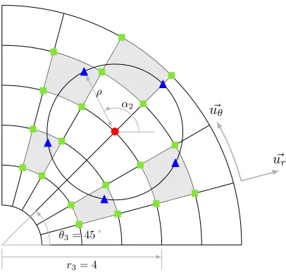
In this section, we describe the computation of the gyroaverage operator in real space developed in [11]. This method implies essentially interpolations over the Larmor circle. Let us consider a functionf discretized over the 2D plane, on which the gyroaverage operator will be applied in this study. We distribute uniformly
N quadrature points on the circle of integration and since the quadrature points do not coincide with grid points, we introduce an interpolation operator P. Fig. 1 gives an example of this approach withN = 5. We have evaluated two schemes: Hermite interpolation and cubic spline interpolation. The gyroaverage is then obtained by the rectangle quadrature formula on these points. More precisely, for a given point (ri, θj) in a
polar coordinate system, the gyroaverage at this point is approximated by
Jρ(f)ri,θj '
1 2π
N−1
X
k=0
P(f)(ricosθj+ρcosαk, risinθj+ρsinαk)∆α, (1)
whereαk=θj+k∆αand ∆α= 2π/N.
When points are outside the domain in the previous sum, we perform a radial projection on the border of the domain:
- ifr < rminthenP(f)(r, θ) is replaced byP(f)(rmin, θ),
- ifr > rmaxthenP(f)(r, θ) is replaced byP(f)(rmax, θ).
~ ur ~
uθ
θ3= 45˚
r3= 4 ρ
α2
•
N N
N
N
N
Figure 1. Description of the gyroaverage based on an interpolation method. One has to
compute the gyroaverage on the red point •. To do that, one estimates the average of the
f function at blue locations N. The f values at blue points are obtained thanks to Hermite interpolation usingf which is known on the mesh points, here particularly at mesh points.
2.2.
Hermite interpolation
The Hermite interpolation method consists in a reconstruction of a polynomial function of degree 3 over a cell of the mesh (filled in light gray on Fig. 1) such that the value and the first derivative of this polynomial are equal to those of the input discretized function on the edges of the cell.
To do this, the values of the derivatives are reconstructed from the nodal values of the function f a finite difference scheme of arbitrary orderd. Regardless of the dvalue, the Hermite polynomial remains of order 3, which allows a flexible use. It is possible to improve the precision of the interpolation by increasing the arbitrary order of the derivative reconstruction. In addition, unlike cubic splines interpolation, the Hermite interpolation method is very local; it requires only very few points close to the target position of the interpolation.
2.2.1. Interpolation over a 1D mesh
We detail here the Hermite interpolation operator in the uni-dimensional case before taking into account the 2D polar coordinate system in the next subsection. Let us consider a domain Ω = [a, b] ⊂R divided intoN
cells:
Ci= [xi, xi+1], withi∈J0, N−1K.
The mesh is assumed uniform, i.e. for any indexi the space step ∆xverifies
∆x=xi+1−xi= b−a
N .
Letα∈[0,1[. The reconstruction off by Hermite interpolation over the cellCi reads:
f(xi+α∆x) ≈(2α+ 1)(1−α)2f(xi) +α2(3−2α)f(xi+1)+
α(1−α)2f0(x+i ) +α2(α−1)f0(x−i+1).
values f(xi+k) around the point xi with a stencil from k = r−d ≤ 0 to k = s
−
d ≥ 0 (resp. k = r +
d ≤ 0 to k=s+d ≥0). More precisely,
f0(x−i )≈Ψ−d(f(xi)), f0(x+i )≈Ψ+d(f(xi))
where the operators Ψ±d :RN+1→RN+1 are:
(Ψ−d(X))i= s−d
X
k=rd−
ωk,d− Xi+k, (Ψ+d(X))i = s+d
X
k=r+ d
ωk,d+ Xi+k
with
ωk,d± =
s±d
Y
j=r±d, j6=k,0
(−j)
s
± d
Y
j=r±d, j6=k
(k−j) ifk6= 0
−
s±d
X
j=r±d, j6=0
ωj,d± else.
For an even reconstruction orderd= 2p, the stencil reads:
rd−=−p, s−d =p, r+d =−p+ 1, s+d =p+ 1
and for an odd orderd= 2p+ 1, we have:
r−d =r+d =−p, s−d =s+d =p+ 1.
We observe that in the case of an odd (resp. even) order, the reconstruction is uncentered (resp. centered) and the reconstructed derivative function is C0 (resp. C1). In the numerical results presented in the following, the default order will bed= 4.
2.2.2. Interpolation over a 2D polar mesh
We consider now an uniform polar mesh over the domain [rmin, rmax]×[0,2π] with Nr×Nθ cells:
Cij= [ri, ri+1]×[θj, θj+1], withi∈J0, Nr−1K, j∈J0, Nθ−1K
where
ri= rmin+irmaxN−rrmin, i∈J0, NrK
θj= jNθ2π, j∈J0, NθK.
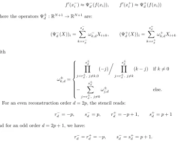
Hermite interpolation over a polar mesh, which corresponds to a tensor product, consists on a succession of one-dimensional Hermite interpolations.
Fig. 2 highlights an intermediate step. On the red points (˜r, θ) and (˜r, θ+ 1), the underlying discretized function f is interpolated to get its value and several derivatives. Then these values are used to evaluate f
at the target point f(˜r,θ˜) generally inside a cell. The interpolation method is summed up by the following algorithm:
- interpolation of the functionf(·, θj) over [ri, ri+1] in order to evaluate f(˜r, θj)
(˜r, θ)
(˜r, θ+ 1)
N
(˜r,θ˜)
Figure 2. Details on the interpolation steps for one point. The pointNinside the cell
repre-sents the target value. It is obtained thanks to the Hermite interpolation between the interme-diate pointsfrom the top and the bottom of the cell.
- interpolation of the function∂θf(·, θ+j) over [ri, ri+1] in order to evaluate ∂θf(˜r, θ+j)
- interpolation of the function∂θf(·, θ−j+1) over [ri, ri+1] in order to evaluate ∂θf(˜r, θ−j+1)
- interpolation of the functionf(˜r,·) over [θj, θj+1] by using the 4 previous evaluations to calculatef(˜r,θ˜).
To achieve these 1D interpolations, we build as a first step the partial derivatives at the cell interfaces:
(∂rf(ri+, θj))i∈J0,NrK ≈ Ψ
+
d(f(ri, θj)i∈J0,NrK) ∀j∈J0, NθK (∂rf(r−i , θj))i∈J0,NrK ≈ Ψ
−
d(f(ri, θj)i∈J0,NrK) ∀j ∈J0, NθK (∂θf(ri, θ+j))j∈J0,NθK ≈ Ψ
+
d(f(ri, θj)j∈J0,NθK) ∀i∈J0, NrK (∂θf(ri, θ−j))j∈J0,NθK ≈ Ψ
−
d(f(ri, θj)j∈J0,NθK) ∀i∈J0, NrK,
then the second derivatives:
(∂r,θ2 f(r+i , θj+))i∈J0,NrK ≈ Ψ
+
d(∂θf(ri, θ +
j)i∈J0,NrK) ∀j∈J0, NθK (∂r,θ2 f(r−i , θj+))i∈J0,NrK ≈ Ψ
−
d(∂θf(ri, θ +
j)i∈J0,NrK) ∀j∈J0, NθK (∂r,θ2 f(r+i , θj−))i∈J0,NrK ≈ Ψ
+
d(∂θf(ri, θ
−
j)i∈J0,NrK) ∀j∈J0, NθK (∂2r,θf(r−i , θj−))i∈J0,NrK ≈ Ψ
−
d(∂θf(ri, θ
−
j)i∈J0,NrK) ∀j∈J0, NθK.
In the general case, for any node (ri, θj), the following 9 values need to be recorded:
f(ri, θj), ∂rf(r+i , θj), ∂rf(ri−, θj), ∂θf(ri, θj+), ∂θf(ri, θ−j)
∂r,θ2 f(ri+, θj+), ∂r,θ2 f(r−i , θ+j), ∂r,θ2 f(r+i , θ−j), ∂2r,θf(r−i , θ−j).
However, in the case of an even orderd, as the reconstructed derivative function isC1, only the four following
values are stored sincer+=r− andθ+=θ−:
2.3.
Analytical test case
To check and verify the gyroaveraging numerical solvers, one can use analytical solutions. For that, we use the Fourier-Bessel functions whose gyroaverage is analytically known [11]. More precisely, for an integerm≥0, letJmandYm be respectively the Bessel functions of the first kind and of the second kind of orderm(see [8]), we consider the following test function which verifies the homogeneous Dirichlet conditions on rmin >0 and rmax:
fm,k: (r, θ)∈[rmin, rmax]×[0,2π]7→
Jm(γm,k)Ym
γm,k r rmax
−Ym(γm,k)Jm
γm,k r rmax
eimθ
whereγm,k is thekthzero of the functiony7→Jm(y)Ym
yrmin
rmax
−Ym(y)Jm
yrmin
rmax
.Its gyroaverage reads:
Jρ(fm,k)(r0, θ0) =J0
γm,k ρ rmax
fm,k(r0, θ0). (3)
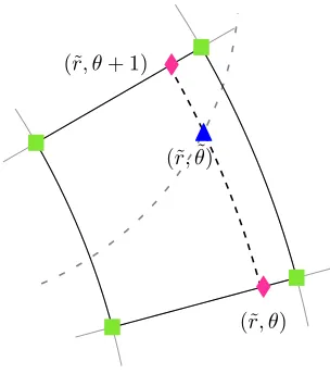
The real and imaginary parts of the functionf1,1is illustrated at Fig. 3.
Figure 3. Real and imaginary parts of the test functionf1,1 withrmin= 1 andrmax= 9.
We designed a unit test which is based on the analysis of the error – the difference between analytical solution and the computed solution (usingL1orL2norm). Setting the gyroradiusρ, the number of points on the Larmor
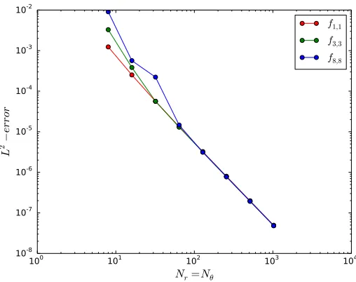
circleN and the interpolation orderd, one can draw the numerical behavior of the error and check the order 2 in space; in practice, we use the real part of these functions. The Fig. 4 shows the L2−error between the analytical gyroaverage and the numerically computed gyroaverage with the three functions f1,1, f3,3 andf8,8
depending on the resolution of the mesh. The higher the modes (m, k) of a function are, the more this function oscillates, which induces larger approximation errors. This explains the observed differences between the curves on Fig. 4 for the lowest values ofNr, Nθ. Starting fromNr=Nθ≥102, the three curves are not distinguishable
any more, which means the resolution of the mesh is fine enough to catch the oscillations of the three functions and so to ensure a good accuracy of the gyroaverage computation.
Another verification consists, for a functionfm,k and a given point (r0, θ0), in calculating the ratio
Jρ(fm,k)(r0, θ0) fm,k(r0, θ0)
≈J0
γm,k ρ
rmax
100 101 102 103 104
Nr=Nθ 10-8
10-7 10-6 10-5 10-4 10-3 10-2
L
2−
er
ro
r
f1,1
f3,3
f8,8
Figure 4. L2-error for the gyroaverage of the real part of the functions f1,1, f3,3 and f8,8
in function of Nr =Nθ. The gyroaverage is computed using the method based on Hermite
interpolation with N = 1024 points on the Larmor circle. Parameters : rmin = 1, rmin = 9, d= 4 andρ= 1.
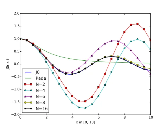
which can be seen as an approximation of the Bessel function J0 thanks to Eq. (3). Fig. 5 illustrates the
reconstruction of J0 using the functionf8,8 withrmin= 1,rmax= 9,Nr=Nθ= 1024, (r0, θ0) has coordinates
(470,470) in the mesh,γ8,8≈36.0 and 0≤ρ≤ 10γr8max,8 ≈2.5. Since the functionf8,8has the highest mode values
among the three considred functions, it is the most difficult function to handle by the gyroaverage operator and so it is relevant to study the error depending on the number of interpolation points. The larger the number
N is, the better the Hermite curves fit the analytical solutionJ0, whereas the Pad´e approximation appears as
rough starting from x= 2.
These unit tests allow us to study the precision of the gyroaverage operator depending on the input parameters but it also represents reference cases. The validity of any new implementation was systematically checked by comparing their results with these unit tests against those of the reference implementation. During the development process, this check warns us early if something goes wrong, it facilitates the fixing of bugs.
3.
Matrix representation for gyroaveraging
3.1.
Matrix description of the gyroaverage operator
The previous section described the gyroaverage computed at a given grid point thanks to Eq. (1). In the case of the even order, this formula boils down to a linear combination of 4 values at the nodal points of the polar mesh: the value, the derivative of first order in the radial and in the poloidal directions, and the cross-derivative of second order (see relation (2)). These values are denotedWf in the following.
0 2 4 6 8 10 x in [0, 10]
2.0 1.5 1.0 0.5 0.0 0.5 1.0 1.5 2.0
J0( x )
J0
Pade
N=2
N=4
N=6
N=8
N=16
Figure 5. Reconstructions of the function J0 using the function f8,8 and its gyroaverage
computed by the method based on Hermite interpolation with N = 2,4,6,8 or 16 points on the Larmor circle. These reconstructions are functions ofx=γ8,8rmaxρ .
used for optimization issues. The gyroaverage based on Hermite interpolation can be written as follows:
Mf inal=Mcoef×Mf val
with
Mf inal ∈ MNr+1,Nθ(R),
Mcoef ∈ MNr+1,4(Nr+1)Nθ(R),
Mf val ∈ M4(Nr+1)Nθ,Nθ(R).
The matrixMf inal is the result of the gyroaverage applied to all the points of a poloidal cut. Every point on this matrix verifies the relation:
Mf inal(i, j) =Jρ(f)ri,θj
with
ri= r
min+irmaxN−rmin
r , i∈J0,NrK,
θj= jNθ2π, j∈J0,Nθ−1K.
The last point in theθdirection is excluded as it shares the same position as the first point in this periodical direction. Each rowRi of the matrixMcoef contains the contribution coefficients associated to the input plan
at a given indexiin the radial direction. The matrixMf valcontains in each columnCj the required values for
Hermite interpolation. The factor 4 which appears in the size of the matrices Mcoef andMf val is due to the
number of required values by the interpolation method over a 2Dplane – 4 per grid point in the Hermite case. With this representation, the gyroaverage computed at one grid point can be expressed as the following scalar dot product:
3.2.
Initial implementation of the gyroaverage operator
For convenience, we will use the matrix-like notations introduced above to describe the initial implementation used in [11]. This implementation does not benefit of the clear identification of the manipulated objects. In the initial implementation of the algorithm, the gyroaverage operator was not seen as a scalar dot product, and so some contribution was not factorized in the most efficient way.
Accordingly to the matrix representation of the gyroaverage, the two main properties of the matrix Mcoef
are(i) the sparsity (section 3.3) and(ii) and the fact that it remains unchanged during the whole simulation. This matrix is computed once for all in the initialization step, whereas the matrix Mf val is computed at each gyroaveraging because the values it contains are determined by the considered input data.
The implementation is composed of two steps: the first at the initialization stage described by Algo. 1 and the second at each call togyro computeduring the simulation run described by Algo. 2.
input : Nr, Nθ,ρ, N
output: A representation ofMcoef – the weights and the indexes of their correspondingWf for eachi. for i ←0 toNrdo
for k←0 toN−1 do
Compute thekthposition of the quadrature pointptover the Larmor circle of center (i, j= 0);
Compute/store the indexes of the corner points of the cellcell containingpt;
Compute/store the weights associated to the contribution of each corner point of cellinto a representation ofMcoef;
end end
Algorithm 1:Computation of a representation ofMcoef (initialization step).
input : Thef values in the poloidal plane input plane
output: The gyroaveraged poloidal plane: gyroaveraged values at each grid point of the poloidal plane for each grid point pt (i,j)of input planedo
Compute/store the first order derivative off in each dir. and the cross-derivative atpt (i,j)into a representation ofC(Mf val);
end
for each point pt (i,j) of input plane do
Compute the gyroaveraged value atpt (i,j)– do the sparse dot productRi(Mcoef)×Cj(Mf val); Store the gyroaveraged value into theinput planeat pt (i,j);
end
Algorithm 2: Computation of the gyroaverage off over a poloidal plane taken as input.
3.3.
Pattern of the matrix
M
coefTo figure out the sparsity of the matrix Mcoef, take a look at Fig. 1 (p. 193). The i-th line of the matrix
Mcoef contains the coefficient contribution of every position of the input poloidal plane for the gyroaverage at a point (i, j=∗). As we can see on Fig. 1, to compute the gyroaverage of the point in the center of the circle (•), only a few points of the plane contribute (). As a consequence, the weight associated to a point of the plan is non-zero for this gyroaverage only if it is used to get the value of an interpolate point (N). This is the case for any mesh point. This leads us to conclude that the matrixMcoef is sparse. The Fig. 6 illustrates the
generic appearance of thei-th line vector ofMcoef.
. . .
α0i,j α1i,j α2i,j α3i,j 0 0 0 0
4(Nr+ 1)Nθ Ri(Mcoef)≡
with
α0
i,j the weight associated to fi,j α1i,j the weight associated to ∂rfi,j α2
i,j the weight associated to ∂θfi,j α3i,j the weight associated to ∂2r,θfi,j
Figure 6. Sketch of the sparsity of a row vectorRi(Mcoef). On this example, only the cells
filled in grey contain non-zero valuesα∗i,j.
in their respective gyroaverage remain the same in local coordinate system along poloidal direction (u~r, u~θ).
The value and the distribution of the α∗i,j coefficients depend only of the radial indexi.
The number of non-zero values of 2 separated row vectors may be different. The pattern of the cells which contribute to the computation of the gyroaverage depends on the radial indexi of the target point. Generally, the target points close to the center of the poloidal mesh (i.e. iis low) involve a larger number of cells compared to the point near to the external boundary of the plane.
3.4.
Pattern of the matrix
M
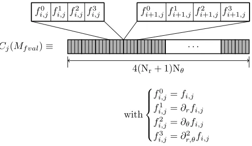
f valThe matrixMf val stores the needed values for the Hermite interpolation, namely the nodal value and their derivatives. The layout of a column of this matrix is illustrated on Fig. 7.
. . .
fi,j0 fi,j1 fi,j2 fi,j3 fi0+1,j fi1+1,j fi2+1,j fi3+1,j
4(Nr+ 1)Nθ Cj(Mf val)≡
with
f0 i,j=fi,j f1
i,j=∂rfi,j f2
i,j=∂θfi,j f3
i,j=∂r,θ2 fi,j
Figure 7. Sketch of the layout of a column vectors ofMf val.
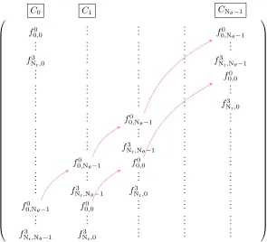
The length of any vectorCj(Mf val) is 4(Nr+ 1)Nθand contains only non-zero values. In the current matrix
representation (see Fig. 8), one can notice thatMf val has a repetitive pattern. The distribution of the values
in a vector Cj(Mf val) depends on its poloidal indexj. The values of the vectorCj+(Mf val) can be obtained
on Fig. 8. From the 1st column vector, the other ones can be deducted thanks to the following relation:
Cj6=(Mf val)[i] =C(Mf val)[i−j×4(Nr+ 1)] (5)
f0
0,0 ... ... ... f00,Nθ−1
..
. ... ... ... ...
fN3r,0 ... ... ... fN3r,Nθ−1
..
. ... ... ... f0
0,0
..
. ... ... ... ...
..
. ... ... ... f3
Nr,0
..
. ... f0
0,Nθ−1
..
. ... ..
. ... ... ... ...
..
. ... f3
Nr,Nθ−1
..
. ... ..
. f0
0,Nθ−1 f 0
0,0 ... ...
..
. ... ... ... ...
..
. f3
Nr,Nθ−1 f 3 Nr,0
..
. ...
f00,N
θ−1 f
0
0,0 ... ... ...
..
. ... ... ... ...
f3
Nr,Nθ−1 f 3 Nr,0
.. . ... ...
C0 C1 CNθ−1
Figure 8. Illustration of the value position shift between the columns ofMf val.
The matrix representation of the gyroaverage operator provided in this Section gives us a useful description. Section 4 details the different optimizations we have made to quicken the initial computation of the gyroaverage thanks to this matrix representation.
4.
Optimize and speedup gyroaveraging
The gyroaverage operator is decomposed into two stages, as already mentioned in section 3.2. Algo. 1 is computed during the initialization step and only once, so its execution time is taken as a payload for the simulation and is not the goal of the optimizations presented here. Algo. 2 is called many times during an iteration of Gyselaand is the main kernel of the gyroaverage operator. The optimizations done focus on the reduction of the execution time of this algorithm. To achieve the optimization of the gyroaverage operator, we paid attention to data structures which represent the matrices involved in the computation. In a second step, issues relative to cache memory levels are tackled.
In this Section, we describe several implementations. The first one that is presented in 4.1 must be seen as the starting point for the optimizations introduced in 4.2 and 4.3.
4.1.
Compact vector optimization
Obviously, the choice of the data structures for the matrixMcoef andMf valhas great impact on the
are taken into account. By avoiding the storage of null values, the size of vectors involved in Eq. (4) is reduced, but it requires the use of dedicated data structures to achieve the computation of Algo. 2.
The main contribution of this optimization is the choice of the data structure that implements the sparse matrix version of the gyroaverage.
During the development process, different data structures were tested. The data structure which represents the matrix Mcoef is less challenging than the representation of the matrix Mf val, since Mf val has a visible impact on performances. Among the different representations ofMf val, two of them are detailed and compared below.
4.1.1. The representation of the matrixMcoef
The goal of the computation of Algo. 1 is to compute the representation of the matrix Mcoef. As said previously, it is done during the initialization step and only once. To benefit of the sparsity of this matrix
Mcoef, a dedicated data structure contribution vector has been created to handle it. This structure is
defined as follows:
1 type :: gyro_vector
2 integer, dimension(:), pointer :: ind
3 real(8), dimension(:), pointer :: val
4 end type gyro_vector
5
6 type(gyro_vector), dimension(:), pointer :: contribution_vector
The variable contribution vector is an array of length (Nr+ 1) and of type gyro vector which is a
structure as defined above. Each cell of contribution vectorrepresents a row vector of the matrix Mcoef.
For a given radial index i, the indexes of the underlying mesh points which contribute to the gyroaverage of the point (i, j = 0) are computed and saved in contribution vector(i)%ind. Its length is denoted by
nb contribution pt(i)and may be different for each radial index (see section 3.3). These indexes are used to build the variable which represents the matrixMf val which will be detailed below. The weights associated to
these positions are computed and stored in contribution vector(i)%val.
4.1.2. First representation of the matrixMf val
Algo. 2 which describes the main kernel of gyroaverage can be decomposed into two parts: (i)the computation of the derivatives and(ii) the computation of the product between the weights and theWf of the input plane. At each call togyro compute, the derivatives of the input plane are computed and saved in a variable denoted
rhs product. This variable represents the matrix Mf val. In this implementation, rhs product is defined as follows:
1 type :: small_matrix
2 real(8), dimension(:, :), pointer :: val
3 end type small_matrix
4
5 type(small_matrix), dimension(:), pointer :: rhs_product
The variablerhs productis an array of length (Nr+ 1); it contains elements of typesmall matrixwhich is
a structure containing simply a 2D pointer. The shape of a 2D arrayrhs product(i)%valis
(4 × nb contribution pt(i), Nθ). This array is the matrix that contains the subset of values from matrix Mf valcontributing to the gyroaverage of the points (i,j=∗). Its first column vector
rhs product(i)%val( :,j = 0) contains the Wf retrieved from the first column vector C(Mf val) which corresponds to the position recorded in the vector contribution vector(i)%ind. The other columns
rhs product(i)%val( :,j 6= 0) are deduced thanks to a shift of j×4(Nr+ 1) positions as one can see in
Fig. 8.
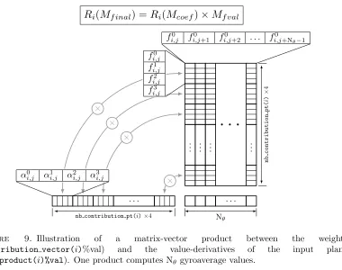
Fig. 9 illustrates the matrix-vector product between the weights and the Wf. Here, theWf from a vector
. . .
.. . ... ...
. . .
.. .
nb contribution pt(i)×4
nb
contribution
pt(
i
)
×
4
×
×
×
× fi,j0
f1
i,j
f2
i,j
f3
i,j fi,j0 f1
i,j f2
i,j f3
i,j
α0
i,j α1i,j α2i,j α3i,j α0
i,j α1i,j α2i,j α3i,j
fi,j0 fi,j0 +1 fi,j0 +2 . . . fi,j0+N θ−1
. . .
Nθ
R
i(
M
f inal) =
R
i(
M
coef)
×
M
f valFigure 9. Illustration of a matrix-vector product between the weights
(contribution vector(i)%val) and the value-derivatives of the input plane
(rhs product(i)%val). One product computes Nθ gyroaverage values.
from the vector contribution vector(i)%val. In this way, the gyroaverage can be implemented as matrix-vector products which are efficient operations on modern processors. Each matrix-matrix-vector product computes the gyroaverage of Nθ points. The gyroaverage of the whole poloidal plane is achieved with (Nr+ 1) matrix-vector
products.
4.1.3. Second representation of the matrixMf val
In this second approach, the variable rhs product is still the representation of the matrix Mf val, but it is
defined as follows:
1 real(8), dimension(:), pointer :: rhs_product
Therhs product variable is here a 1D array. It corresponds exactly to the first column vectorC(Mf val).
As said in Section 3.4, this vector contains all theWf deduced from the input plane, so its length is 4(Nr+ 1)Nθ.
One can see it as the linear flat representation of the input plane.
Fig. 10 shows the product between the weights and theWf accordingly to this representation. The length
of the vectors involved in this product does not match. The association between weights and theWf is done thanks to the position recorded in the vector contribution vector(i)%ind. This association is graphically represented by the arrows. The gyroaverages of points (i,j6= 0) are computed thanks to a shift of 4j(Nr+ 1)
of the indexes from contribution vector(i)%ind. This operation will be called sparse dot product in the following.
To achieve the gyroaverage of the whole poloidal plane, (Nr+ 1)Nθ sparse dot products are required.
4.1.4. Benchmark to compare the data structures
. . .
.. .
nb contribution pt(i)×4
(N
r
+
1)
×
Nθ
×
4
×
×
×
× fi,j0 fi,j1
f2
i,j
f3
i,j fi,j0 fi,j1 f2
i,j f3
i,j
α0
i,j α1i,j α2i,j α3i,j α0
i,j α1i,j α2i,j α3i,j
contribution
vector(i)%ind
M
f inal(
i, j
) =
R
i(
M
coef)
×
C
j(
M
f val)
Figure 10. Illustration of the sparse dot product between the weigths
(contribution vector(i)%val) and the value-derivatives of the input plane (rhs product). The matching between these two arrays is done thanks to the position recorded in
contribution vector(i)%ind.
Nr=Nθ 32 64 128 256 512
RHS 1,5·10−3 1,1·10−2 8,5·10−2 5,1 ·10−1 2,3
Structure 1: Product 2,1·10−4 1,7·10−3 1,4·10−2 8,3 ·10−2 3,5·10−1
Total 1,7·10−3 1,3·10−2 9,9·10−2 5,9 ·10−1 2,7 RHS 1,7·10−4 6,4·10−4 2,5·10−3 1,0 ·10−2 4,2·10−2
Structure 2: Product 7,9·10−4 5,7·10−3 4,6·10−2 2,7 ·10−1 1,2
Total 9,7·10−4 6,3·10−3 4,9·10−2 2,8 ·10−1 1,3
Table 1. Comparison of performance of the 2 data structures on the analytical test case.
Structure 1 corresponds to the first representation of Mf val (described in section 4.1.2) and structure 2 to the second one (described in section 4.1.3). The execution times are given in seconds. They result from the average over 100 runs. (ρ = 0.05, rmin = 0.1, rmax = 0.9,
N = 32).
the complexity comp(Nr, Nθ) representing the product between the weights and the Wf as the number of
multiplications involved. In our case, it reads as follows:
comp(Nr, Nθ)= Nr X
i=0
4×nb contribution pt(i)×Nθ.
This relation highlights the strong correlation between the number of grid points and the time complexity of the gyroaverage.
Section 2.3. The time corresponding to the building of the variable rhs productis given in lines ”RHS” and the time for the product between the weights and theWf in lines ”Product”.
The second data structure implementation is roughly twice faster than the first one. If you pay attention to the details, the first data structure is competitive during the ”Product” step, but the time needed to build the
rhs product represents a large overhead. As the second data structure gives shorter execution times, this is the chosen implementation.
With this data structure, the accesses to the Wf are not contiguous during the sparse dot product (see Fig. 10). This is due to the irregular stencil required by the gyroaverage (see Fig. 1) and to the layout of the variablerhs product. This constitutes a limit for this approach from the performance point of view.
The second data structure is trickier to manipulate for the sparse dot product as it is shown in Section 4.1.3, but it allows us to have the control on the internal data distribution which is the key point for the ”layout optimization” (details in Section 4.3).
To achieve the gyroaverage of the whole plane, at each grid point, a sparse dot product has to be done. In the implementation on the current ”compact vector optimization”, the poloidal plan is covered thanks to 2 nested for-loop where j is the index of the internal loop. Geometrically, the plan is explored circle after circle, from the smaller to the larger ones. This access pattern has the property to extensively reuse the weights (contribution vector). Although this property, it constitutes a limit for performance and represents the key point of the next optimization. We will refer to this access pattern to cover the plane as the mesh path in the next sections.
4.2.
Blocking optimization
As said previously, to achieve the gyroaverage of the whole poloidal plane, a sparse dot product must be done on every grid point. The ”blocking optimization” extends the ”compact vector optimization” implementation. This optimization is focused on the improvement of the access patternmesh path to the input plan inspired by the well-known blocking/tiling technique [12].
To improve the performance, the idea here is to follow a path over the grid pointsmesh path which reduces the frequencies of cache misses during the computation. For any mesh point (i, j), the computation of the gyroaverage required data fromcontribution vector(i)andrhs product. As said in 4.1, doing the gyroaver-age circle after circle ensures a good reuse of the weightscontribution vector(i), but this is not the case for
rhs product. The access to its data is generally not contiguous and differs for 2 distinct mesh points. However, as the data are retrieved by cache line, the cachehit rate depends of themesh path1. The goal achieved in this optimization is to increase the reuse of the data available in cache along themesh path.
Instead of covering the poloidal plan circle after circle, the plan is covered using small 2Dtiles in this version. These tiles are of sizeBLOCKr×BLOCKθand are numbered following the poloidal direction. Fig. 11 illustrates the tiling decomposition of a part of the poloidal mesh. On this sample, BLOCKr = 3 and BLOCKθ = 4. In practice, the setting of BLOCKr and BLOCKθ are tuned depending on benchmarks performed on each
production machine.
The poloidal plane is partitioned intoN Tr×N Tθ tiles. The tiles are numbered along the poloidal direction,
from the center to the outside of the plane. This mesh path cut in tiles improves the temporal locality of the data from the array rhs product. It increases the cachehit rate and so decreases the execution time.
4.3.
Layout optimization
As for the ”blocking optimization”, the ”compact vector optimization” is the starting point of this imple-mentation. Especially, themesh path remains the same in the present implementation. Here, this optimization focuses on the order of the data in the array rhs product. For a given mesh path, the arrangement of these values has a strong impact on the execution time. We will refer to this arrangement of data as the layout of
rhs product.
• •
•
• •
•
• • •
• • •
T ile0 T ile0 T ile1
T ile1 T ileT ileN TN Tθθ
Figure 11. Sample of the tiling technique over a part of the poloidal mesh. The tiles which
partition the mesh are traveled in ascending order. The nested arrows inside a tile show the underlying order.
The optimization of the layout is done for a givenmesh path over the input plane. The access history to the data of rhs productdepends on themesh path. The idea of the optimization presented here is to permute the elements of rhs product, so change its layout, in order to increase the cachehit ratio along themesh path.
The mesh path must be seen as an input parameter of the problem. Depending on the gyroradius ρ, the number of cells Nr×Nθ, the number of points on the Larmor circle N and the mesh path, the access history
to the arrayrhs productis known. To determine how to change the layout, we need to introduce a metric of temporal distance of access of its data.
contribution point list of temporal indexes temporal average (0, 0) [0, 1, 8, 9, 10, 17] 7.0 (0, 1) [0, 1, 8, 9, 10, 17, 18, 19, 26] 12.0 (0, 2) [9, 10, 17, 18, 19, 26, 27, 28, 35] 21.0 (0, 3) [18, 19, 26, 27, 28, 35, 36, 37, 44] 30.0
..
. ... ...
(1, 0) [0, 1, 2, 9, 10, 11] 5.0 ..
. ... ...
Table 2. For each mesh point, list of the indexes corresponding to their use along themesh path
and average of this temporal indexes.
To compute the gyroaverage at a point (i,j), theWf values of its neighborhood are required. The points of this neighborhood are the contribution points to the gyroaverage at the point (i,j). To achieve the gyroaverage of a whole poloidal plan, we compute the gyroaverage of each mesh point one after an other. Let thetemporal index be the index of a grid point along themesh path. For each point of the plane, we have listed the temporal indexes corresponding to the gyroaverages in which it is involved.
contribution point, which is denoted temporal average. For example, thetemporal average of the point (0,0)
is computed as follows:
temporal average((0,0)) = 0 + 1 + 8 + 9 + 10 + 17
6 = 7.
Letpt1a mesh point. If itstemporal average is rather low, this meanspt1contributes rather in the beginning of themesh path. On the opposite, if thetemporal average of a mesh pointpt2is rather high compared to the other temporal averages, this meanspt2contributes rather in the end of themesh path.
The heuristic implemented in this optimization is to sort the elements of rhs product accordingly to their
temporal average. For instance, from the information available on Tab. 2 the resulting partial data layout of
rhs product is: [ (1, 0), (0, 0), (0, 1), (0, 2), (0, 3), . . . ]. The main idea is to keep accessed data between 2 successive sparse dot products as near as possible in order to minimize in average the number of cache misses. In practice, the computation of the new layout of rhs productis done during the initialization step. This implies that the mesh path over the plane must be known at this step. The matching between the weights (contribution vector()%val) and theWf (rhs product) during a sparse dot product is done thanks to the indexes retrieved from the array contribution vector()%ind. To ensure the validity of the computation, the indexes recorded in arraycontribution vector()%indmust be updated accordingly to this new layout.
5.
Performance results in Gysela
5.1.
Benchmarking small cases
After integration of the different versions of the gyroaverage operator in Gysela code [5], different runs have been done to compare their effectiveness. To keep a reasonably short execution time, the simulations are composed of only four time steps. These tests were done on the Helios2 machine. Computation nodes used are equipped with two Intel Xeon E5-2450 2.10GHz processors, so 16 cores a node. On Tab. 3, the different test cases have been performed over the two following meshes (6) and (7):
Nr= 256, Nθ= 256, Nϕ= 32, Nvk= 16, Nµ= 4 (6)
Nr= 512, Nθ= 512, Nϕ= 32, Nvk= 16, Nµ= 4. (7) To highlight the difference of performance between the different gyroaverage implementations, the size of the poloidal plane is multiplied by 4 between the two meshes. For these runs, every gyroaverage based of Hermite interpolation hasN= 16 quadrature points on the integration circle. This number of integration points ensures a good presicion of the results as you can see on Tab. 5. The fluctuation of execution times (several percents typically, but rare events can lead to 10% or 20%) due to shared resources such as network and parallel file system is avoided using a specific configuration. Only one computation node of Helios is used for each run in order not to share the network. Also, the writing and reading on the parallel file system is reduced to the minimum. The benchmark configuration of one run is the following: 16 MPI processes composed of only 1
OpenMP thread. This benchmark corresponds to an execution of only four time steps of Gysela of a non
physical case. This quite artificial setting will be revised in the next Subsection dedicated to production runs. Tab. 3 shows some results concerning the Pad´e approximation compared to 4 versions of the Hermite im-plementation: original implementation; compact vector (described in Section 4.1), blocking (Section 4.2) and layout (Section 4.3) optimizations. Also, the Gysela code can be executed without any gyroaverage at all (solution named Disable gives invalid results of course but consitutes a reference execution time). This last option allows us to determine accurately the fraction of the execution time corresponding to the gyroaverage operator over the total execution time for the other cases.
As expected, the computation time of the gyroaverage operator grows along with the size of the poloidal mesh. The compact vector optimization which were an intermediate step during the optimization process is
Gyroaverage method
Pad´e Hermite Disable
Initial Compact vector Layout Blocking
Mesh (6): Total execution time (sec.) 110,20 150,60 146,35 132,91 131,39 106,18
Percentage of gyroavg. execution 3.8 % 41.8 % 37.8 % 25.2 % 23.7 % –
Mesh (7): Total execution time (sec.) 464,62 629,46 627,80 557,49 550,38 433,35
Percentage of gyroavg. execution 7.2 % 45.3 % 44.9 % 28.6 % 27.0 % –
Table 3. Execution time and percentage over the total time of the gyroaverage operator for
the different versions (for two different mesh sizes of poloidal plane withN = 16 interpolation points).
already a little bit faster than the original implementation. However, the percentage of total execution time dedicated to gyroaverage operator is about 6 to 10 times higher than for the Pad´e approximation. Thelayout optimization offers a great speed up compared to this previous step. On the biggest mesh, it reduces the execution by several tens of percents compared to thecompact vector optimization. This demonstrates the big impact of the data layout in memory.
The best result is obtained with the blocking optimization which reduces the accumulated gyroaverage cost by 40% compared to the initial version. Nevertheless, it is still approximately 4 times more costly than the Pad´e approximation on the largest mesh. This is partly due to the numberN of points used on the integration circle.
Gyroaverage method
Pad´e Hermite Disable
Initial Compact vector Layout Blocking
Mesh (6): Total execution time (sec.) 110,00 131,42 129,11 123,12 120,47 105,60
Percentage of gyroavg. execution 4.2 % 24.4 % 22.3 % 16.6 % 14.1 % –
Mesh (7): Total execution time (sec.) 464,20 544,07 538,38 525,21 510,44 433,49
Percentage of gyroavg. execution 7.1 % 25.5 % 24.2 % 21.2 % 17.8 % –
Table 4. Execution time and percentage over the total time of the gyroaverage operator for
the different versions (for two different mesh sizes of poloidal plane withN = 8 interpolation points).
On Tab. 4, the same simulations have been run with less quadrature points, soN= 8. As expected, reducing
N induces smaller computation costs and decreases the execution times. With twice less quadrature points, the gyroaverage based on Hermite (blocking) reduces its execution time by 40%. Also the gap between theblocking optimization and the Pad´e approximation is reduced. However the drawback of taking less interpolation points leads to a subtle degradation of the quality of the gyroaverage operator. The trade-off between precision and computation will be discussed in the Subsection below.
5.2.
Benchmarking a real-life case
Let us consider a regular domain size and a set of commonly used input parameters to analyze the performance of the new gyroaverage operator on a real-life case. The execution times will be a little bit tainted by network and parallel file system usage, because they are shared by several users. We have launched the simulations several times to ensure the execution times we get are reproducible. We focus on a Cyclone DIII-D base case, with a most unstable mode at (m, n) = (14,−10) and the following parameters: µmin = 0.143, µmax = 7.,
code. In order to check the good behavior of the simulation, a classical verification procedure is to focus on the linear phase and to extract the growth rate of the most unstable mode.
In the literature (see for example [2], p. 39-40), some theoretical and applied works have pointed out that taking N= 8 points to discretize the gyroaverage operator is often sufficient. It has also been shown that this choice is already better than Pad´e to approximate the Bessel function J0(k⊥ρi) on the intervalk⊥ρi ∈ [0,5].
Working with N= 16 points to evaluate the gyroaverage extends the capability of the Hermite interpolation which is now able to accurately approximate the Bessel function on a larger intervalk⊥ρi∈[0,10]. Fig. 5 also
corroborates this fact by an illustration on the specific functionf8,8.
Method Pad´e Hermite
N=2 N=3 N=4 N=6 N=8 N=16
Growth rate γ .10436 .12246 .09420 .09625 .09643 .09644 .09644
Table 5. Linear growth rate for the different versions of the gyroaverage operator on a Cyclone
test case (normalized growth rate as Fig. 1 of [4]).
On Tab. 5, the linear growth rates (normalized as in [4], Fig. 1) observed in the described use case are presented. They characterize the behavior of all the main components of the code during the linear phase. One can see that the values given by Hermite method for N= 6,N= 8,N= 16 are almost equal, which is a good result that shows that simulations are well converged. The asymptotic value is reached quickly as N grows. However, forN= 2,N= 3 and for the Pad´e method, the growth rate is not well recovered. Practically, N= 8 should be taken for production runs and this is a good cost-quality balance. The N= 16 configuration will be useful also in specific cases where great accuracy is wanted by physicists (whenever particles withk⊥ρi>5 play
a major role).
Hermite
Code part\Method Pad´e N=8 N=16
Initial Layout Blocking Initial Layout Blocking
Field solver 28s (0%) 32s (+14%) 31s (+10%) 31s (+11%) 35s (+27%) 32s (+13%) 32s (+16%)
Diagnostics 96s (0%) 123s (+29%) 108s (+12%) 110s (+15%) 147s (+54%) 114s (+19%) 120s (+26%)
Total 629s (0%) 662s (+5.3%) 659s (+4.8%) 651s (+3.6%) 689s (+9.6%) 670s (+6.6%) 666s (+5.8%)
Table 6. Cumulative execution time for some parts of the code that are impacted by
gyroav-erage computation costs. Timings are given for a run of 60 time steps using 512 cores. In parentheses, the percentage of extra time compared to Pad´e reference time is given.
6.
Conclusion
To achieve the optimization of the gyroaverage operator, 4 steps have been achieved: (i) derive numerical approximation of the gyroaverage operator,(ii)describe formally the operator thanks to a matrix representation,
(iii)explore and evaluate different optimization techniques, and(iv)integrate and validate these optimizations in theGyselacode. The current best implementation with Hermite interpolation is twice faster than the initial one. This improvement, but also the enhanced accuracy of the gyroaverage based on Hermite interpolation foster us to use the new solution in production runs instead of the Pad´e approximation.
The Pad´e gyroaverage implementation required a whole poloidal cut as input, due to a Fourier transform in θ direction and to a finite difference discretization along r direction. This involves sometimes collective communications to redistribute the data before applying the gyroaverage, because the main parallel domain decomposition is alongr,θ andµdirections inGysela. Historically, this was a hard constraint because Pad´e was the single solution available in Gysela for gyroaveraging. The new gyroaverage based on interpolation methods circumvents this issue. Parallelizing among severalMPIprocesses will, from now on, be greatly eased. Additionally this new way to compute the gyroaverage allows us to consider easily its extension over general geometry meshes (not only polar planes).
References
[1] J. Bigot, V. Grandgirard, G. Latu, Ch. Passeron, F. Rozar, and O. Thomine. Scaling gysela code beyond 32k-cores on bluegene/q. InCEMRACS 2012, volume 43 ofESAIM: Proc., pages 117–135, Luminy, France, 2013.
[2] I. Broemstrup.Advanced Lagrangian Simulation Algorithms for Magnetized Plasma Turbulence. PhD thesis, Univ. of Mary-land, 2008.
[3] N. Crouseilles, M. Mehrenberger, and H. Sellama. Numerical solution of the gyroaverage operator for the finite gyroradius guiding-center model.Commun. Comput. Phys., 8, 2010.
[4] A. M. Dimits et al. Comparisons and physics basis of tokamak transport models and turbulence simulations.Physics of Plasmas, 7(3):969–983, 2000.
[5] V. Grandgirard, J. Abiteboul, J. Bigot, T. Cartier-Michaud, N. Crouseilles, Ch. Erhlacher, D. Esteve, G. Dif-Pradalier, X. Garbet, Ph. Ghendrih, G. Latu, M. Mehrenberger, C. Norscini, Ch. Passeron, F. Rozar, Y. Sarazin, A. Strugarek, E. Son-nendr¨ucker, and D. Zarzoso. A 5D gyrokinetic full-f global semi-lagrangian code for flux-driven ion turbulence simulations. working paper or preprint, July 2015.
[6] V. Grandgirard, M. Brunetti, P. Bertrand, N. Besse, X. Garbet, Ph. Ghendrih, G. Manfredi, Y. Sarazin, O. Sauter, E. Son-nendr¨ucker, J. Vaclavik, and L. Villard. A drift-kinetic semi-lagrangian 4d code for ion turbulence simulation. Journal of Computational Physics, 217(2):395 – 423, 2006.
[7] V. Grandgirard, Y. Sarazin, P. Angelino, A. Bottino, N. Crouseilles, G. Darmet, G. Dif-Pradalier, X. Garbet, Ph. Ghendrih, S. Jolliet, G. Latu, E. Sonnendr¨ucker, and L. Villard. Global full-f gyrokinetic simulations of plasma turbulence. Plasma Physics and Controlled Fusion, 49(12B):B173, 2007.
[8] M. Kreh. Bessel functions.Lecture Notes, Penn State-G¨ottingen Summer School on Number Theory, 2012.
[9] G. Latu, V. Grandgirard, N. Crouseilles, and G. Dif-Pradalier. Scalable quasineutral solver for gyrokinetic simulation. Research Report RR-7611, INRIA, May 2012.
[10] J. Li. General explicit difference formulas for numerical differentiation.Journal of Computational and Applied Mathematics, 183(1):29–52, 2005.
[11] C. Steiner, M. Mehrenberger, N. Crouseilles, V. Grandgirard, G. Latu, and F. Rozar. Gyroaverage operator for a polar mesh.
The European Physical Journal D, 69(1), 2015.
[12] M. E. Wolf and M. S. Lam. A data locality optimizing algorithm.SIGPLAN Not., 26(6):30–44, May 1991.