N. Champagnat, T. Leli`evre, A. Nouy, Editors
REDUCED BASIS APPROXIMATION FOR THE STRUCTURAL-ACOUSTIC
DESIGN BASED ON ENERGY FINITE ELEMENT ANALYSIS (RB-EFEA)
Denis Devaud
1and Gianluigi Rozza
2Abstract. In many engineering applications, the investigation of the vibro-acoustic response of struc-tures is of great interest. Hence, great effort has been dedicated to improve methods in this field in the last twenty years. Classical techniques have the main drawback that they become unaffordable when high frequency impact waves are considered. In that sense, the Energy Finite Element Analysis (EFEA) is a good alternative to those methods. Based on an approximate model, EFEA gives time and locally space-averaged energy densities and has been proven to yield accurate results.
However, when dealing with structural-acoustic design, it is necessary to obtain the energy density varying a large number of parameters. It is computationally unaffordable and too expensive to compute such solutions for each set of parameters. To prevent this drawback, we introduce a reduced order model which allows to drastically decrease those computational costs, while yielding a reliable and accurate approximation. In this paper, we present an approximation of the EFEA solution considering the Reduced Basis (RB) method. The RB method has already been applied successfully to many different problems. A complete development of this procedure in the context of EFEA is introduced here. Numerical tests and examples are provided for both geometrical and physical parameters.
1.
Introduction and Motivation
In many engineering applications, it is important to be able to compute the acoustic response of built-up structures. This is of particular interest in structural-acoustic design where noise control is desirable. At high frequency, wavelenghts are small compared to the size of the domain, which yields prohibitively large computational costs using standard techniques. Moreover, the response is highly dependent on the space location and frequency. This phenomenon may prevent from catching the general behavior of the structure. For these reasons, it is necessary to develop methods that are able to predict average results.
The most widely used method is the Statistical Energy Analysis (SEA) [6, 13]. In SEA, the first step is to divide the whole system in subsystems consisting of similar resonant modes. Then, the different subsystems are coupled assuming that the difference in their modal energies is proportional to the power flow. The propor-tionality constants are related to the coupling loss factors. However, the assumptions considered to derive such method does not allow to capture spatial variation within a subsystem. Moreover, the input data are usually not consistent with the geometry data bases. Two other exact methods, the General Energetic Method (GEM) and the Simplified Energy Method (SEM) [11], can be used to predict the energy behaviour of structures.
1 EPFL SMA, CH-1015, Lausanne, Switzerland. This work has been carried out during a pre-doc visiting period of the first
author at SISSA Mathlab, International School for Advanced Studies, Trieste, Italy.
2SISSA, International School for Advanced Studies, Mathlab, Via Bonomea 265, 34136 Trieste, Italy;[email protected]. SISSA NOFYSAS Excellent grant and INdAM GNCS are kindly acknowledged.
©EDP Sciences, SMAI 2015
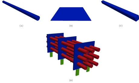
An alternative to the SEA to predict average behaviour is the Energy Finite Element method (EFEA) [4,15]. The main idea is to derive differential equations governing the time and locally space-averaged energy density in continuous structures based on approximate energy models. Such work was first conducted in the 1970s by Belov and Rybak who developed transport equations in vibrating plates [2] and conduction-like equations in ribbed plates [3]. Based on this, Nefske and Sung [18] introduced a so-called power flow finite element method but without investigating the difference between the exact solution and their approximation. In the 1990s, much work has been performed on that topic. The first scientists to address this question were Wohlever and Bernhard [30] who rigorously showed that these approximations were valids for isolated rods and beams. The method has then been extended to infinite and finite plates by Bouthier and Bernhard [5]. In Figure 1, examples of plates, rods, beams and a complete structure are presented. Those three elementary components constitute the main building blocks for many structures and then it is of interest to consider coupling between these components. The firsts to treat this problem were Cho and Bernhard [7,8] who analyzed coupled beams. Recent works have dealt with more complex structures, as for instance in [26]. EFEA methods have been developed to deal with composite structures by Yan [31] and Lee [12]. Finally, a method to approximate the vibro-acoustic response of structures under fluid loading have been introduced by Zhang, Wang and Vlahopoulos [34] for plates and Zhang, Vlahopoulos and Wu [32] for cylindrical shells.
The various EFEA methods have been successfully applied to several engineering problems. Wang and Bernhard have applied the method to heavy equipment cab [28, 29]. The case of a NASA test-bed cylinder has been considered by Wang, Vlahopoulos, Buehrle and Klos [27]. An EFEA method has also been applied to composite aircraft structures by Vlahopoulos, Schiller and Lee [25]. The case of ship structures has been addressed by Zhang, Wang and Vlahopoulos [33] and Vlahopoulos, Garzia-Rios and Mollo [24].
We are interested in obtaining a rapid and reliable evaluation of an output functional depending on the solution computed by the EFEA. It is not desirable to compute a new finite element (FE) solution for each physical or geometrical parameter since it would be computationally unaffordable. Hence, among several option in reduced order modelling, we consider the reduced basis method (RB) [19,20,23] to obtain such approximation by a Galerkin projection. While writing the differential equations associated to the EFEA in a parameter dependent form, we construct the RB approximation of its solution. In particular, we consider classical a posteriori error estimators and the usualOffline-Onlinedecomposition.
The work is organized as follows. In Section 2, we show the complete derivation of the differential equations associated to the EFEA in a simple setting. The generalization to more general cases is straightforward and is based on the ingredients introduced in Section 2.2. A brief survey of the RB method is done in Section 3. In particular, the EFEA equations are written in a parameter dependent form, which is necessary to use the RB method. The Offline-Online procedure as well as a posteriori error estimators for the compliant case are introduced. We also present the complete derivation for parameter-dependent geometries in two-dimensional spaces. Finally, two numerical examples are considered in Section 4. The first one illustrates a crack in a material and uses geometrical parameters. In that case, we are interested in capturing and studying the behaviour of the energy density where the crack occurs. The second one is used to investigate the response of a thin plate to a point impact for different material properties. Some conclusions follow.
2.
Energy Finite Element Analysis
The prediction of vibro-acoustic response is of interest in many engineering applications. However at high frequencies, classical techniques are no more affordable. In fact, when the wavelenghts are short, the mesh needs to be fine to obtain good approximations. Moreover, in that case, the energy density contains many oscillations which prevents from capturing the underlying general behaviour of the response.
(a) (b) (c)
(d)
Figure 1. Examples of domain for (a) rods, (b) plates and (c) beams. Those components
represent the basis of many more complicated structures such as (d). For this reason, the first EFEA models were derived while considering computational domains with such shapes and then composite structures were investigated.
We present here a complete development leading to the differential equations which are the basis of EFEA. This is done in a simple framework by considering a single thin plate. Models for other single material component structures are also introduced.
2.1.
Derivation of EFEA equations for plates
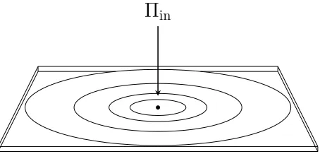
In this section, we introduce an EFEA for a single finite volume Ω surrounded by a surface ∂Ω; see for instance [5, 15]. The main point is the derivation of the energy equation, which is a differential equation. We consider the simple case of a flexural wave applied to a finite plate as depicted in Figure 2. This special situation has been studied by Bouthier and Bernhard [5]. The reason for considering such component is that it is the basis for many structures of interest in structural-acoustic design. In fact, ships, aicrafts and cars are good examples of the necessity to study vibro-acoustic responses of plates. In that setting, we have the following equation for the energy densityE:
− ∇ · c 2 g
ηω∇E
!
+ηωE=πin, in Ω, (2.1)
the medium under consideration. We use (2.1) to introduce our RB approximation, in particular to derive the weak formulation, but the derivation follows the same lines for equations associated to other medium. More general models can be obtained considering a different transmission equation, such as those in [30] for rods and beams. Such relations are introduced in the next section. Moroever, (2.1) is only valid for a simple element but coupled structures can be considered; see for instance [8].
Π
inFigure 2. Example of flexural wave applied to a thin finite plate simulating a local impact.
We assume thatcg,η andω are constant and strictly positive over the whole domain. To obtain the weak formulation of our problem, we impose that the energy vanishes on the boundary, that is E = 0 on∂Ω. The function space for E is then X := H01(Ω), i.e. the Sobolev space of square integrable functions with square integrable gradients that vanish on the boundary ∂Ω. The weak formulation of (2.1) follows using standard techniques: findE∈H01(Ω) such that
c2 g
ηω
Z
Ω
∇E· ∇v+ηω
Z
Ω
Ev=
Z
Ω
πinv, ∀v∈H01(Ω). (2.2)
Note that it is possible to consider piecewise constant values forcg,η andω. In that case, we write
Ω = Kdom
[
k=1
Ωk, (2.3)
with Ωk∩Ωl =∅ for 1≤k < l≤Kdom. The constants cg,k, ηk andωk represent the values ofcg, η andω on Ωk, respectively. The weak formulation of (2.1) then becomes: findE∈H01(Ω) such that
Kdom
X
k=1
c2 g,k
ηkωk
Z
Ωk
∇E· ∇v+ηkωk
Z
Ωk
Ev
!
=
Z
Ω
πinv, ∀v∈H01(Ω). (2.4)
2.2.
Equations for other types of structural components
As already pointed in Section 1, plates, rods and beams are the basis for many different structures. It is then of interest to derive equations such as (2.1) for these structural components. This is discussed here following [30]. The three main ingredients in order to obtain (2.1) are
(1) an energy balance equation; (2) an energy loss relationship;
(3) a transmission equation bridging the intensity and the energy density.
waves. In all cases, the transmission equation is of the form
I=−c 2 g
ηω∇E,
where Iis the energy flow through the boundary. However, the type of impact wave considered modifies the value of the group speed. For plates and beams, we use flexural impact waves and so
cg= 2
ω2D
ρh
1/4
, (2.5)
where D is the bending stiffness of the material, ρits density and hthe thickness of the plate. In the case of rods, longitudinal vibrations are considered and so
cg=
s
G
ρ, (2.6)
whereGis the shear modulus of the rod.
3.
Reduced Basis Approximation for the Energy Finite Element Method
For each value of the constantscg,η andω, a different energy densityE(cg, η, ω) is obtained. It also depends on the shape of the computational domain considered. In many applications, it is of particular interest to investigate different material properties and shapes. However, it is unaffordable to compute a new solution for each input parameter and so we consider a reduced order model [14, 19, 20, 23] to reduce those computational costs. It is for instance very important if we want to perform optimization on the material properties and more particularly structural-acoustic design. This goal is achieved here by considering a RB approximation of the FE solution of the EFEA equation (2.2). The RB method has already been proven to be very efficient in many different engineering problems.
3.1.
Data Preprocessing and Finite Element Approximation
To be able to construct a RB approximation of E(cg, η, ω), the first step is to write (2.2) in a parameter-dependent form. The brief methodological development here follows mainly [19, 20, 23] and a complete survey of the RB method can be found in those references. The reader interested in the application of RB method in material modelling and linear elasticity may refer to [17] as a preliminary work. The parameter of interest is defined in our case as µ = (cg, η, ω) ∈ D ⊂ R3, but other physical and geometrical parameters could be
considered, the important parameter-dependent domain option is presented in Section 3.5. For instance, in the case of a thin plate, it would be interesting to consider the density and the Young’s modulus as parameters instead of the group speedcgdefined by (2.5). To be able to apply the RB method, we write (2.2) in an abstract setting
a(E, v;µ) =f(v;µ), ∀v∈H01(Ω), (3.1) wherea(·,·;µ) andf(·;µ) depend affinely on µ, that is
a(E, v;µ) = Qa
X
q=1
Θqa(µ)aq(E, v), (3.2)
f(v;µ) = Qf
X
q=1
The assumptions (3.2) and (3.3) are crucial for the derivation of the method. It allows the algorithm to be splitted in two different computational steps, the so-called Offline and Online ones. The main goal is to obtain computational costs in the Online stage which are independent of the FE space dimension. This is achieved considering the affine decomposition. If the affine decomposition assumption is not fulfilled, the empirical interpolation method [1] can be used to derive the separate representations (3.2) and (3.3) approximately.
We are interested in the following problem: for µ∈ D, evaluate
s(µ) =l(E(µ)), (3.4)
where E(µ)∈H1
0(Ω) is the solution of (3.1) andl :H01(Ω)→Ris a continuous and linear functional. In fact, in many applications, it is of particular interest to know the average energy density in particular areas of the domain. This gives crucial informations when dealing with structural-acoustic design.
Turning now to the special case of EFEA and considering (2.2), we haveQa = 2,Qf = 1 and
Θ1a(µ) =
c2 g
ηω, a
1(E, v) =
Z
Ω
∇E· ∇v,
Θ2a(µ) =ηω, a2(E, v) =
Z
Ω
Ev,
Θ1f(µ) = 1, f1(v) =
Z
Ω
πinv,
which implies thatf(v;µ) = f(v) is parameter-independent. The previous equations may be extended to the case of piecewise constant parameters (2.4) by considering the same affine decomposition on each subdomain. This leads to Qa = 2Kdom and Qf = Kdom terms. Note that a(E, v;µ) = a(v, E;µ) for all E, v ∈ H01(Ω) and µ∈ D, i.e. ais a symmetric operator. The continuity and coercivity constants associated toa(·,·;µ) are defined as
γ(µ) := sup v∈H1
0(Ω),v6=0
sup w∈H1
0(Ω),w6=0
a(v, w;µ) kvkkwk ,
and
α(µ) := inf v∈H1
0(Ω),v6=0
a(v, v;µ) kvk2 ,
where kvk :=kvkH1 0(Ω) :=
R
Ω(∇v) 212
is the norm considered onH01(Ω). Since ais continuous and coercive, there exists 0 < α0 ≤ γ0 < ∞ such that α0 ≤α(µ) ≤ γ(µ)≤ γ0 for allµ ∈ D. This guarantees the well-posedness of (2.2) if f is continuous. To ensure its continuity, we assume that πin ∈ L2(Ω). For a sake of simplicity, we choose f = l, which is called, together with the fact that a is symmetric, the compliant case assumption. The non-compliant case is treated in [23].
LetXN ⊂H01(Ω) be a (conforming) FE space ofH01(Ω) with dim(XN) =N <∞. We then consider a FE approximation of (3.4): given µ∈ D, evaluate
sN(µ) =l(EN(µ)), (3.5)
whereEN(µ)∈XN ⊂H01(Ω) is the solution of
a(EN(µ), v;µ) =f(v), ∀v∈XN. (3.6)
We define the associated continuity and coercivity constantsγN(µ) andαN(µ) as
γN(µ) := sup v∈XN,v6=0
sup w∈XN,w6=0
and
αN(µ) := inf v∈XN,v6=0
a(v, v;µ) kvk2 .
Due to the conforming hypothesis, it follows that α(µ) ≤αN(µ)≤γN(µ) ≤γ(µ), ∀µ∈ D. It implies that the FE formulation (3.6) is well-posed. We have now all the ingredients to introduce the RB approximation of (3.5)-(3.6). This is done in the next section.
3.2.
Reduced Basis Method
As it has already been pointed out, it is computationally unaffordable to compute a new FE solution for every input parameter µ. The goal of the RB method is then to approximate the FE solution EN(µ) with reduced computational costs. ConsideringN sufficiently large, we have thatEN(µ) is close enough toE(µ) in a certain norm so that the FE approximation can be viewed as the “truth” solution.
Given a positive integer Nmax N, we construct a sequence of hierarchical approximation spaces
X1N ⊂X2N ⊂ · · · ⊂XNNmax⊂XN. (3.7)
Those spaces are obtained considering a Greedy algorithm presented more in details in Section 3.3. The hieriarchial hypothesis (3.7) is important to ensure the efficiency of the method. Several spaces can be considered to construct such sequence, but they all focus on the smooth parametric manifoldMN :=
EN(µ)µ∈ D .
If it is smooth enough, we can expect it to be well approximated by low-dimensional spaces. In what follows, we consider the special case of Lagrange reduced basis spaces built properly selecting a master set of parameter points µn ∈ D, 1 ≤ n ≤ N
max. Other examples such as the POD spaces [23] could be considered. For 1≤N≤Nmax, we defineSN :=
µ1, . . . ,µN and the associated Lagrange RB spaces
XNN := span
EN(µn)1≤n≤N .
The selection of the snapshots EN(µn) is one of the crucial points of the RB method and is further inves-tigated in the next section. Due to possible colinearity, we apply the Gram-Schmidt process in the (·,·)X inner product to the snapshots EN(µn) to obtain mutually orthonormal functions ζnN. In that case, we have
XNN = spanζnN1≤n≤N . Since colinearities are avoided using the Gram-Schmidt orthonormalization
process, we are ensured that the dimension N obtained is minimal. The RB approximation of the problem (3.5)-(3.6) is obtained considering Galerkin projection: givenµ∈ D, evaluate
sNN(µ) =f(ENN(µ)), (3.8)
whereENN(µ)∈XNN is the solution of
a(ENN(µ), v;µ) =f(v), ∀v∈XNN. (3.9)
Sincef =l andais symmetric, we obtain
sN(µ)−sNN(µ) =kEN(µ)−ENN(µ)k2
µ, (3.10)
wherek · kµ := p
a(·,·;µ) is the energy norm induced by the inner product a(·,·;µ) (sinceais symmetric and coercive). In Section 3.4, we present an example of inexpensive and efficient a posteriori error estimator ∆N(µ) for kEN(µ)−EN
N(µ)kµ on which the Greedy algorithm is based. Due to the relation (3.10), it is possible to
SinceENN(µ)∈XNN = span
ζnN1≤n≤N , we extend it as
ENN(µ) = N
X
m=1
EN,mN (µ)ζmN. (3.11)
The unknowns then become the coefficientsEN,mN (µ). Inserting (3.11) in (3.8) and (3.9) and using the hypothesis that f is linear andabilinear, we obtain
sNN(µ) = N
X
m=1
EN,mN (µ)f(ζmN),
and
N
X
m=1
EN,mN (µ)a(ζmN, ζnN;µ) =f(ζnN), 1≤n≤N. (3.12)
The stiffness matrix associated to the system (3.12) is of size N ×N with N ≤ Nmax N. It yields a considerably smaller computational effort than to solve the system associated to (3.6), whose matrix is of size N × N. However, the construction of the stiffness matrix involves the computation of theζmN associated with theN-dimensional FE space.
This drawback is avoided by constructing an Offline-Online procedure taking advantage of the affine decom-postion (3.2). In the Offline stage, the Greedy algorithm is used to construct the set of selected parametersSN. Then, theEN(µn) and theζnN are built for 1≤n≤N. Thef(ζnN) andaq(ζmN, ζnN) are also formed and stored. Note the importance here of the affine decomposition (or some surrogates of it). It implies that the vector and matrices stored are independent of the input parameterµ.
In the Online part, the stiffness matrix associated to (3.12) is assembled considering the affine decomposition (3.2). This yields
a(ζmN, ζnN;µ) = Qa
X
q=1
Θqa(µ)aq(ζmN, ζnN), 1≤m, n≤N.
The same process is applied to the right-hand sidef. TheN×N system (3.9) is then solved to obtainEN,mN (µ), 1≤m≤N. Finally, the output of interest (3.8) is computed considering the coefficients obtained.
As already discussed, one of the main feature of the RB method is that we have a posteriori error estimators ∆N(µ) forkEN(µ)−ENN(µ)kµ and so easily also for the output errorsN(µ)−sNN(µ) whose computation costs are independent ofN. It allows us to certify our method and make it reliable. A discussion on such estimators is presented in Section 3.4.
3.3.
Greedy Algorithm for the Snapshots Selection
One of the most important step taking place in the Offline stage is the wisely selection of the parametersµn, 1 ≤n ≤N. Several algorithms are available in the literature [23] but we introduce here a greedy procedure for completeness. The general idea of this procedure is to retain at iterationN the snapshot EN(µN) whose approximation provided byXN−1N is the worst one. Let us assume that we are given a finite sample of points Ξ⊂ D and pick randomly a first parameterµ1∈Ξ. Then forN = 2, . . . , N
max, compute
µN := arg max
µ∈Ξ∆N−1(µ),
where ∆N(µ) is a sharp and inexpensive a posteriori error estimator forkEN(µ)−ENN(µ)kH1
0(Ω)orkE
N(µ)−
EN
N(µ)kµ. The algorithm is typically stopped when ∆N(µ) is smaller than a prescribed tolerance for every
Since XN−1N ⊂XNN, we expect to have ∆N(µ)≤∆N−1(µ), which ensures that Nmax<∞. The derivation of ∆N(µ) is crucial for the Greedy and we introduce an example of such estimator in the next section.
3.4.
A posteriori error estimators for elliptic coercive partial differential equations
The basic ingredient of the Greedy algorithm procedure is the computable error estimator, which has to be independent of N. In fact, it is used also online to certify that the error of our RB approximation with respect to the truth solution is under control. For completeness, the derivation of such estimator is only recalled here when the compliant case is considered, i.e. a is symmetric and f = l [22]. Let us introduce the error
eN(µ) =uN(µ)−uNN(µ)∈XN which satisfies the following equation
a(eN(µ), v;µ) =f(v;µ)−a(uNN(µ), v;µ) =:r(v;µ), (3.13)
wherer(·;µ)∈ XN0
is the residual and XN0
denotes the dual space ofXN. To define our a posteriori error estimator, we need to have a lower bound αNLB(µ) of αN(µ) such that 0< αLBN (µ)≤αN(µ)∀µ∈ D and the online costs to computeαNLB(µ) are independent ofN. We then define the following a posteriori error estimator
∆N(µ) :=
kr(·;µ)k(XN)0 αNLB(µ) .
To computekr(·;µ)k0
(XN), the main ingredients are: (i) the affine assumption (3.2) onaand (ii) the expansion
(3.11) of ENN(µ) in the space XNN. Then, using the definition (3.13) of the residual, this leads to a system depending only on N for everyµ, which makes the computation independent ofN.
The procedure used to compute the coercivity lower bound αNLB(µ) is the so-called Successive Constraint Method (SCM) [10]. Considering sets based on parameter samples and the terms Θaq of the affine decomposition (3.2), it is possible to reduce this problem to a linear optimization problem. This method works by taking into account neighbor informations for the parametrized stability factors and its precision increases with the size of the neighborhood considered. The SCM also creates a coercivity upper bound αNUB(µ) of αN(µ) in the same manner. The algorithm is stopped when maxµ∈Ξ αNUB(µ)−αLBN (µ)/αNUB(µ)
is smaller than a prescribed toleranceε.
We emphasize on the fact that it is very important that the costs associated to the computation of ∆N are independent of N. That allows us to develop the Offline-Online procedure discussed in Section 3.2 which is a crucial ingredient of the reduced basis method and its efficiency.
3.5.
Parameter-Dependent Domain Geometry
The derivation of the reduced basis approximation of energy finite element solutions may be performed under the assumption that the domain Ω is not parameter-independent. In many applications we may consider that the domain is parametrized such that Ωo= Ωo(µ). The notation Ωo stands for “original domain”, which is the computational one. Here µ denotes the vector containing the physical parameterscg, η andω as well as the parameters defining the geometry. The parameter-dependent case is recalled here from [19].
Considering the decomposition (2.3), we write
Ωo(µ) = Kdom
[
k=1
Ωko(µ),
with Ωk
(3.2). We require that for every 1≤k≤Kdom, there exists an affine mappingTk(·;µ) : Ωk→Ωko(µ) such that
Ωko(µ) =Tk(Ωk;µ).
The mappingsTk(·;µ) have to be bijective and collectively continuous, that is
Tk(x;µ) =Tl(x;µ), ∀x∈Ωk∩Ωl, 1≤k < l≤K dom.
Note that the decomposition is independent of the FE approximation and so Kdom does not depend on N. Based on these mappings, we construct a global transformation T as
T(x;µ) :=Tk(x;µ), k= minn1≤l≤K dom
x∈Ω
lo
.
The mappingT is globally bijective and piecewise affine. The choice of the minimum is arbitrary and could be chosen differently.
More explicitly, we define the affine mappings Tk for everyx∈Ωk andµ∈ Das
Tk(x;µ) :=Ck(µ) +Gk(µ)x,
where Ck : D →
Rd and Gk : D →Rd×d for every 1 ≤k ≤Kdom, represent a translation and a rotation of the subdomain, respectively. To define the affine decomposition of the bilinear form a, we need to define the Jacobians and the inverse of the rotational transformationsGk(µ) as
Jk(µ) := |det(Gk(µ))|,
Dk(µ) := Gk(µ)−1
,
for 1≤k≤Kdom.
Based on what have been introduced, we explicitly give the affine decomposition (3.2) of the bilinear forma
in the cased= 2. The three dimensional case is obtained in a similar way [9]. Let us denoteAk
o(µ) the matrix
Ako(µ) :=
c2g,k
ηkωk 0 0 0 c
2
g,k
ηkωk 0 0 0 ηkωk
, such that
ao(E, v;µ) = Kdom
X
k=1
Z
Ωk o(µ)
h
∂E ∂x1
∂E ∂x2 E
i
Ako(µ)
∂v ∂x1 ∂v ∂x2 v ,
where (x1, x2)∈ Ωo(µ) and ao denotes the bilinear form on the original domain. The bilinear form a on the reference domain can then be expressed [19] as
a(E, v;µ) = Kdom X k=1 Z Ωk h ∂E ∂x1 ∂E ∂x2 E
i
Ak(µ)
where
Ak(µ) =Jk(µ)Dk(µ)Ak o(µ)(D
k(µ))T, (3.14)
with
Dk(µ) :=
Dk(µ) 0 0 0 0 1
.
Developing explicitly (3.14), we obtain the following affine decomposition for every 1≤k≤Kdom:
Θ1,ka (µ) = c 2 g,k
ηkωk (Gk
1,2(µ))2+ (Gk2,2(µ))2
Jk(µ) ,
Θ2,ka (µ) = − c 2 g,k
ηkωk
Gk
2,1(µ)Gk2,2(µ) +Gk1,1(µ)Gk1,2(µ)
Jk(µ) ,
Θ3,ka (µ) = − c 2 g,k
ηkωk
Gk2,1(µ)Gk2,2(µ) +Gk1,1(µ)Gk1,2(µ)
Jk(µ) ,
Θ4,ka (µ) = c 2 g,k
ηkωk (Gk
2,1(µ))2+ (Gk1,1(µ))2
Jk(µ) ,
Θ5,ka (µ) = Jk(µ)ηkωk, Θ1,kf (µ) = Jk(µ),
a1,k(E, v) =
Z Ωk ∂E ∂x1 ∂v ∂x1 ,
a2,k(E, v) =
Z Ωk ∂E ∂x1 ∂v ∂x2 ,
a3,k(E, v) =
Z Ωk ∂E ∂x2 ∂v ∂x1 ,
a4,k(E, v) =
Z Ωk ∂E ∂x2 ∂v ∂x2 ,
a5,k(E, v) =
Z
Ωk
Ev,
f1,k(v) =
Z
Ωk
πinv,
whereGk
i,j(µ) := (Gk(µ))i,j. Note that considering such expansion, we obtainQa= 5Kdom andQf=Kdom terms in the affine decompositions (3.2) and (3.3), respectively.
4.
Numerical Results
In this section, we present two numerical applications of the method introduced in this paper, combining RB and EFEA. All simulations have been performed using the rbMIT [21] library in MATLAB [16].
In the first example, we consider a domain in which a crack in the material occurs. The goal is to predict the average vibro-acoustic response of the material in such a case and particularly the behaviour of the energy density around the crack and it can be seen as a diagnosis tool to detect material defects. This first case is used to illustrate the method when considering geometrical parameters.
The second example illustrates the average response of a thin plate to a localized shock. In that case, we apply a pointwise load on a thin plate. We see that the damping is more considerable when the frequency increases. The parameters considered here are only physical and are the group speed associated to the flexural wave and its frequency.
4.1.
Material Crack
The first example that we consider is used to investigate the behaviour of the energy density when a crack or defect in the material occurs. The computational domain is depicted in Figure 3. The crack dimension varies as
µ1∈[0.5,4.5], while the upper layer between the crack and the top is prametrized byµ2 ∈[1,5]. We consider only geometrical parameters and the physical ones are kept constant to the following values
• cg= 5.127·103 m/s; • η= 0.01;
• ω= 3000 Hz.
while homogeneous Neumann ones are used for the rest of the boundary. Since we consider longitudinal wave in this case, we have thatcg is of the form (2.6), which is
cg=
s
G
ρ, (4.1)
whereG= 7·1010 N/m2 is the shear modulus of the material andρ= 2700 kg/m3its density. In this case we consider a piece of alloy.
(µ1,0)
(0, µ2) (5, µ2)
(0,−5) (5,−5)
Ω
Figure 3. Computational domain for the crack case. The dashed line corresponds to the
boundary on which unitary Neumann conditions apply. We consider non-homogenous Dirichlet b.c. on the bottom side to simulate a longitudinal impact wave. Homogeneous Neumann conditions are imposed on the rest of the boundary.
Turning to the computational results, we obtainN = 2462 basis functions for the FE space andN = 17 for the RB one. The computational time associated to the FE computation for the parameter µ= (1,1) is 33 s. We consider a sample of 100 parameter values and compute the average time necessary for the RB evaluation. In this case, 0.15 s are necessary in average to obtain a RB approximation. Finally, the whole offline process necessites 305 s. It means that the use of the RB method is justified as soon as more than 10 evaluations are desired. We present in Figure 4 some representative solutions for different parameter values. The shape of the domain is kept constant while the size of the crack is increased. It appears that when its size increases, the jump of the solution increases as well. This is confirmed by the curves presented in Figure 6. The convergence of the a posteriori error estimator is depicted in Figure 5 considering a log-scale. In that case, we plot the maximum value of the estimator on the sample with respect toN, that is maxµ∈Ξ∆N(µ). The a posteriori error estimator used here for the computation is the one introduced in Section 3.4 and we considered the Greedy algorithm together with the SCM for the computation of the coercivity lower bound.
Finally, we present in Figure 6 the value of the energy density along the line x = 0.7. The solution is presented for different values ofµ1whileµ2= 2 is kept constant. The reason for observating the solution along this line is that it crosses the crack whenµ1 increases and it allows us to exactly capture the behaviour of the energy density with respect to the break when it occurs and cross the virtual line represented by x= 0.7. For
(a) (b) (c)
Figure 4. Energy density (dB) for the crack problem with the following parameters : (a) µ1= (0.5,2), (b)µ2= (1,2) and (c) µ3 = (2,2). We see that the jump of the energy density in the region of the crack increases with the propagation of the flaw in the domain.
Figure 5. Convergence of the a posteriori error estimator for the crack problem. The
maximum value of the estimator taken over the whole sample is plotted against N, that is maxµ∈Ξ∆N(µ).
Figure 6. Energy density (dB) of the crack case along the linex= 0.7 for several values of
the parameterµ1. The parameterµ2= 2 is kept fixed. We investigate here the implication of the crack on the energy density. The values in the legend correspond to those of µ1, which is the size of the crack.
4.2.
Localized impact on a thin plate
The domain considered in this example is a thin plate of size 20 m×20 m×0.2 m. A force term is applied on the center of the material to simulate a localized pointwise impact. In such case, we are interested in investigating the vibro-acoustic response of the plate for different material properties and frequencies of the impact wave. Hence, only physical parameters are considered and the domain is kept fixed for all parameters. The situation is the one depicted in Figure 2. Since the damping loss factor η appears in equation (2.2) as a product with the frequencyω, we keep it fixed atη= 0.01 and vary onlyω. The other parameter considered is the velocity speed, which takes the form (2.5) for plates and flexural waves, that is
cg= 2
ω2D
ρh
1/4
.
In our case,h= 0.2 m is the thickness of the plate. It means that varyingcgimplies that eitherDorρchanges. It would be possible to consider one of those parameters instead ofcg. The ranges for our parameters are the following ones
• cg∈[100 m/s,200 m/s]; • ω∈[500 Hz,2000 Hz].
The magnitude of the impact flexural wave is 1 N. As the model used gives a locally space and time-averaged energy density, we expect the solution to behave in a smooth manner even for high frequencies. For the model, we consider homogeneous Neumann on the whole boundary, which corresponds to zero flux.
The computation is such thatN = 2744 degrees of freedom for the FE space, while the RB one only contains
solution on the planez= 0.1 m forω = 2000 Hz andcg= 141 m/s. The solution shown is the RB one and it has the smooth behaviour expected. Moreover, we see that the energy density given in dB does not have a big range of variation.
Figure 7. Energy density (dB) of the thin plate problem obtained for the planez = 0.1 m
withω= 2000 Hz andcg= 141 m/s. The pick of the energy is situated at the localized point impact of the flexural wave.
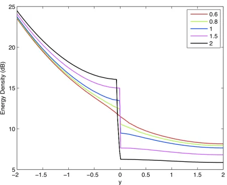
The next results represent the energy density along the line {(x, y, z)∈Ω|x= 10, z= 0.1} and are repre-sented in Figure 8. The first curve depicts the energy density for several frequencies andcg= 100. We see that at low frequencies, the maximal value is high and decreases while the frequency considered increases. When the frequency reaches ω = 1000 Hz, this phenomenon is reverted and the maximum value increases with the frequency. We see that at 500 and 2000 Hz, the pick corresponds to the same energy. It would be interesting to investigate further and do the same test for even higher frequencies. Another important feature that can be observed is that the minimum value of the energy density in the plate decreases when the frequency increases. It means that the damping is more important at high frequencies.
We find the same behaviour in the second curve, which corresponds to the solution for cg = 200. In that case, the maximum value of the energy density only decreases and does not reincrease after a threshold as in the case cg= 100. It would also be interesting to compute approximations for higher frequencies to see if such threshold exists but has not been reached in the considered range of frequencies. Another difference with the previous curve is that the magnitude of the damping is smaller here. We see that, at low frequencies, there is nearly no damping, which is not the case forcg= 100.
Finally, in both cases the maximum is reached at the center of the domain, which is the location where the point impact is located. This is the behaviour expected because it means that the acoustic response is more important where the force is applied on the material.
5.
Conclusions
(a)
(b)
Figure 8. Energy density (dB) for the thin plate problem along the line
{(x, y, z)∈Ω| x= 10, z= 0.1} for different frequency values and (a) cg = 100 and (b)
find approximated smooth solutions of the energy density to understand the vibro-acoustic response of different materials. Such equation has been shown for thin plates and other structural components have been introduced. In many applications it is of interest to obtain EFEA solutions for different parameter values. Hence, we have then presented a RB approximation of the EFEA to obtain a solution for different parameters in the model in an inexpensive and reliable way with significant computational savings. One of the reason to use such method is to be able to perform optimization, analysis and diagnosis on the considered structure with reasonable computational costs (real-time computing and many query contexts). Finally, we have presented two numerical examples. The first one contained a propagating crack in the material, while the second one represented the reaction of a thin plate to a localized shock. These models are very useful for diagnostics and non-destructive material evaluations, combined, for example, with material modelling and structural design.
Acknowledgements
SISSA NOFYSAS excellence grant and SISSA Pre-Doc Program are kindly acknowledged for the support provided at the International School for Advanced Studies, Trieste, Italy, as well as INdAM-GNCS.
References
[1] M. Barrault, Y. Maday, N. Nguyen, and A. Patera,An ’empirical interpolation’ method: application to efficient
reduced-basis discretization of partial differential equations, Comptes Rendus Mathematique, 339 (2004), pp. 667–672.
[2] V. Belov and S. Ryback,Applicability of the transport equation in the one-dimensional wave propagation problem, Journal of Soviet Physics Acoustics, 21 (1975), pp. 173–180.
[3] V. Belov, S. Rybak, and B. Tartakovskii,Propagation of vibrational energy in absorbing structures, Journal of Soviet Physics Acoustics, 23 (1977), pp. 115–119.
[4] R. Bernhard and J. Huff,Structural-acoustic design at high frequency using the energy finite element method, Journal of Vibration and Acoustics, 121 (1999), pp. 295–301.
[5] O. Bouthier and R. Bernhard, Simple models of the energetics of transversely vibrating plates, Journal of Sound and Vibration, 182 (1995), pp. 149–164.
[6] C. Burroughs, R. Fischer, and F. Kern,An introduction to statistical energy analysis, The Journal of the Acoustical Society of America, 101 (1997), pp. 1779–1789.
[7] P. Cho,Energy flow analysis of coupled structures, (1993).
[8] P. Cho and R. Bernhard,Energy flow analysis of coupled beams, Journal of Sound and Vibration, 211 (1998), pp. 593–605. [9] F. Gelsomino and G. Rozza,Comparison and combination of reduced-order modelling techniques in 3d parametrized heat
transfer problems, Mathematical and Computer Modelling of Dynamical Systems, 17 (2011), pp. 371–394.
[10] D. Huynh, G. Rozza, S. Sen, and A. Patera, A successive constraint linear optimization method for lower bounds of
parametric coercivity and inf-sup stability constants, Comptes Rendus Mathematique, 345 (2007), pp. 473–478.
[11] Y. Lase, M. Ichchou, and L. Jezequel,Energy flow analysis of bars and beams: theoretical formulations, Journal of Sound
and Vibration, 192 (1996), pp. 281–305.
[12] S. Lee,Energy Finite Element Method for High Frequency Vibration Analysis of Composite Rotorcraft Structures, PhD thesis, The University of Michigan, 2010.
[13] R. Lyon, R. DeJong, and M. Heckl,Theory and application of statistical energy analysis, The Journal of the Acoustical Society of America, 98 (1995), pp. 3021–3021.
[14] A. Manzoni, A. Quarteroni, and G. Rozza,Computational reduction for parametrized PDEs: strategies and applications, Milan Journal of Mathematics, 80 (2012), pp. 283–309.
[15] S. Marburg and B. Nolte,Computational acoustics of noise propagation in fluids: finite and boundary element methods, Springer, 2008.
[16] MATLAB,version 7.10.0 (R2010b), The MathWorks Inc., Natick, Massachusetts, 2010.
[17] R. Milani, A. Quarteroni, and G. Rozza, Reduced basis method for linear elasticity problems with many parameters, Computer Methods in Applied Mechanics and Engineering, 197 (2008), pp. 4812 – 4829.
[18] D. Nefske and S. Sung,Power flow finite element analysis of dynamic systems: basic theory and application to beams, Journal of Vibration Acoustics Stress and Reliability in Design, 111 (1989), p. 94.
[19] A. Patera and G. Rozza,Reduced basis approximation and a posteriori error estimation for parametrized partial differential equations, MIT, Pappalardo Monograph in Mechanical Engineering, http://augustine.mit.edu, 2007.
[20] A. Quarteroni, G. Rozza, and A. Manzoni, Certified reduced basis approximation for parametrized partial differential
[21] rbMIT Software, Copyright MIT, D.B.P. Huynh, N.C. Nguyen, A.T. Patera and G. Rozza, 2007-09. Web address for
download: http://augustine.mit.edu/.
[22] G. Rozza,Reduced-basis methods for elliptic equations in sub-domains with a posteriori error bounds and adaptivity, Applied Numerical Mathematics, 55 (2005), pp. 403–424.
[23] G. Rozza, D. Huynh, and A. Patera,Reduced basis approximation and a posteriori error estimation for affinely parametrized elliptic coercive partial differential equations, Archives of Computational Methods in Engineering, 15 (2008), pp. 229–275. [24] N. Vlahopoulos, L. Garza-Rios, and C. Mollo,Numerical implementation, validation, and marine applications of an
energy finite element formulation, Journal of Ship Research, 43 (1999), pp. 143–156.
[25] N. Vlahopoulos, N. Schiller, and S. Lee,Energy finite element analysis developments for vibration analysis of composite aircraft structures, SAE International Journal of Aerospace, 4 (2011), pp. 593–601.
[26] N. Vlahopoulos, A. Wang, and K. Wu,An efea formulation for computing structural response of complex structures, ASME, 2005.
[27] A. Wang, N. Vlahopoulos, R. Buehrle, and J. Klos,Energy finite-element analysis of the nasa aluminum test-bed cylinder, The Journal of the Acoustical Society of America, 119 (2006), p. 3389.
[28] S. Wang,High frequency energy flow analysis methods: Numerical implementation, applications, and verification, (2000). [29] S. Wang and R. Bernhard,The energy finite element method applied to a heavy equipment cab, 1998 (1998), pp. 682–687. [30] J. Wohlever and R. Bernhard,Mechanical energy flow models of rods and beams, Journal of Sound and Vibration, 153
(1992), pp. 1–19.
[31] X. Yan,Energy finite element analysis developments for high frequency vibration analysis of composite structures, PhD thesis,
The University of Michigan, 2008.
[32] W. Zhang, N. Vlahopoulos, and K. Wu, An energy finite element formulation for high-frequency vibration analysis of externally fluid-loaded cylindrical shells with periodic circumferential stiffeners subjected to axi-symmetric excitation, Journal of Sound and Vibration, 282 (2005), pp. 679–700.
[33] W. Zhang, A. Wang, and N. Vlahopoulos,An alternative energy finite element formulation based on incoherent orthogonal waves and its validation for marine structures, Finite Elements in Analysis and Design, 38 (2002), pp. 1095–1113.