3D DISCRETE WAVELET TRANSFORM VLSI
ARCHITECTURE FOR IMAGE PROCESSING
Akshayraj Zala
M.Tech. (Digital communication) Indus University, Ahmedabad,India [email protected]
ABSTRACT
In this paper, we propose an improved version of lifting based 3D Discrete Wavelet Transform (DWT) VLSI architecture which uses bi-orthogonal 9/7 filter processing. This is implemented in FPGA by using VHDL codes. The lifting based DWT architecture has the advantage of lower computational complexities transforming signals with extension and regular data flow. This is suitable for VLSI implementation. It uses a cascade combination of three 1-D wavelet transform along with a set of in-chip memory buffers between the stages. These units are simulated, synthesized and optimized by Xilinx 12.1 and MATLAB 7.9 tools.
INTRODUCTION
First of all, why do we need a transformation or what is a transformation anyway? Mathematical transformations are applied to raw signals to obtain further information from that signal which is not readily available in that raw signal. In this paper, I will assume that the time domain signals as raw signals and a signal that has been transformed by any of the available mathematical transformation is called processed signal [1, 7 and 8].
1. Fourier Transform :
Most of the signals in the practice are time domain signals in their raw format. That is, whatever that signal is measuring is a function of time. When we plot time domain signals, we obtain a time-amplitude representation of the signal. This representation is not always the best representation of the signal for most of the signal processing related applications. In many cases, the most distinguished information is hidden in the frequency content of the signal. The frequency spectrum of the signal shows what frequencies exist in the signal. So, by Fourier Transform we can find the frequency content of the signal by below Equation.
Now, two types of signal systems are available. First one is stationary signal system and another one is non-stationary signal system. Here first we examine the stationary signal system by an example which is given below:
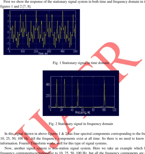
First we show the response of the stationary signal system in both time and frequency domain in the below figures 1 and 2 [7, 8].
Fig. 1 Stationary signal in time domain
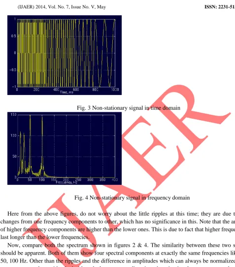
Fig. 2 Stationary signal in frequency domain
In this signal shown in above figures 1 & 2 has four spectral components corresponding to the frequencies 10, 25, 50, 100 Hz. All the frequency components exist at all time. So there is no need to know any time information. Fourier Transform works well for this type of signal systems.
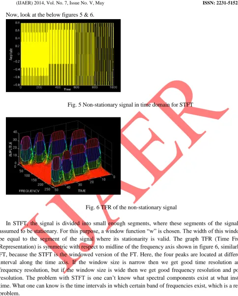
Fig. 3 Non-stationary signal in time domain
Fig. 4 Non-stationary signal in frequency domain
Here from the above figures, do not worry about the little ripples at this time; they are due to sudden changes from one frequency components to other, which has no significance in this. Note that the amplitudes of higher frequency components are higher than the lower ones. This is due to fact that higher frequencies are last longer than the lower frequencies.
Now, compare both the spectrum shown in figures 2 & 4. The similarity between these two spectrums should be apparent. Both of them show four spectral components at exactly the same frequencies like 10, 25, 50, 100 Hz. Other than the ripples and the difference in amplitudes which can always be normalized, the two spectrums are almost identical although the corresponding time-domain signals are not even close to each other. So, Fourier Transform gives the spectral content of the signal only, but it gives no information regarding where in time domain those spectral components appear. Therefore, FT is not suitable technique for non-stationary signal.
2. Short Time Fourier Transform (STFT) :
Now, look at the below figures 5 & 6.
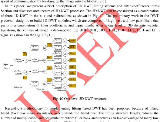
Fig. 5 Non-stationary signal in time domain for STFT
Fig. 6 TFR of the non-stationary signal
3. Wavelet Transform :
Now, Wavelet Transform has two parts one is Continuous Wavelet Transform (CWT) and Discrete Wavelet Transform (DWT). Now, first we will discuss about CWT.
a) Continuous Wavelet Transform (CWT):
Now, to overcome with the problem of time-frequency resolution, it is possible to analyze any signal by using an alternative approach called the multiresolution analysis (MRA). MRA is designed to give good time resolution and poor frequency resolution at high frequencies and good frequency resolution and poor time resolution at low frequencies. Look at the below figure 7 & 8. [7, 8]
Fig. 7 Non-stationary signal in time domain for Wavelet
Fig. 8 Wavelet Transform of non-stationary signal
As seen in the above equation, the transformed signal is a function of two variables, and s, the translation and scale parameters, respectively. Ψ (t) is the transforming function, and it is called the mother wavelet. The term wavelet means a small wave. The smallness refers to the condition that this (window) function is of finite length (compactly supported). The wave refers to the condition that this function is oscillatory. The term mother implies that the functions with different region of support that are used in the transformation process are derived from one main function, or the mother wavelet. In other words, the mother wavelet is a prototype for generating the other window functions.The term translation is used in the same sense as it was used in the STFT; it is related to the location of the window, as the window is shifted through the signal. This term, obviously, corresponds to time information in the transform domain. Scale in the wavelet analysis is similar to the scale used in maps. Higher scales correspond to a non-detailed global view for low frequency components and low scale corresponds to a detailed view for high frequency components.
b) Discrete Wavelet Transform (DWT):
Although the discretised continuous wavelet transform enables the computation of the continuous wavelet transform by computers, it is not a true discrete transform. As a matter of fact, the wavelet series is simply a sampled version of the CWT, and the information it provides is highly redundant as far as the reconstruction of the signal is concerned.In the discrete case, filters of different cut-off frequencies are used to analyse the signal at different scales. The signal is passed through a series of high pass filters to analyse the high frequencies, and it is passed through a series of lowpass filters to analyse the low frequencies. [1-7]
Fig. 9 One level of transformation
Now similarly shown in the figure 9, multiple levels (scales) are made by repeating the filtering and decimation process on low-pass and high-pass outputs. [7]
3D DISCRETE WAVELET TRANSFORM WITH LIFTING SCHEME
Recent advances in medical imaging and telecommunication systems require efficient speed, resolution and real-time memory optimization with maximum hardware utilization. The 3D DiscreteWavelet Transform (DWT) is widely used method for these medical imaging systems because of perfect reconstruction property. DWT can decompose the signals into different sub bands with both time and frequency information. DWT architecture, in general, reduces the memory requirements and increases the speed of communication by breaking up the image into the blocks. [2-5]
In this paper, we present a brief description of 3D DWT, lifting scheme and filter coefficients inthis Section and discusses architecture of 3D DWT processor. The 3D DWT can be considered as a combination of three 1D DWT in the x, y and z directions, as shown in Fig. 10. The preliminary work in the DWT processor design is to build 1D DWT modules, which are composed of high-pass and low-pass filters that perform a convolution of filter coefficients and input pixels. After a one-level of 3D discrete wavelet transform, the volume of image is decomposed into HHH, HHL, HLH, HLL, LHH, LHL, LLH and LLL signals as shown in the Fig. 10. [1]
Fig. 10 One-level 3D DWT structure
Recently, a methodology for implementing lifting based DWT has been proposed because of lifting based DWT has many advantages over convolution based one. The lifting structure largely reduces the number of multiplication and accumulation where filter bank architectures can take advantage of many low power constant multiplication algorithms. FPGA is used in general in these systems due to low cost and high computing speed with reprogrammable property.
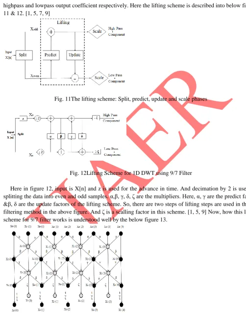
highpass and lowpass output coefficient respectively. Here the lifting scheme is described into below figures 11 & 12. [1, 5, 7, 9]
Fig. 11The lifting scheme: Split, predict, update and scale phases
Fig. 12Lifting Scheme for 1D DWT using 9/7 Filter
Here in figure 12, input is X[n] and z is used for the advance in time. And decimation by 2 is used for splitting the data into even and odd samples. α,β, γ, δ, δ are the multipliers. Here, α, γ are the predict factors &β, δ are the update factors of the lifting scheme. So, there are two steps of lifting steps are used in the 9/7 filtering method in the above figure. And δ is a scalling factor in this scheme. [1, 5, 9] Now, how this lifting scheme for 9/7 filter works is understood well by the below figure 13.
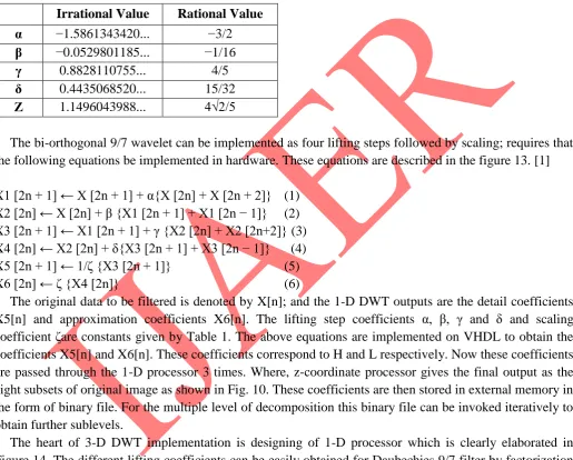
Table 1 shows the irrational and approximated rational counterpart for 9/7 filter which are considered as a very good alternative to irrational coefficients. When these coefficients are applied to image coding, the compression performance is almost same as that of irrationalized filter coefficient implementation, while the computational complexity is reduced remarkably. [1, 5, 9]
Table 1: Irrational and rational lifting coefficients for 9/7 wavelet transform
Irrational Value Rational Value
α −1.5861343420... −3/2
β −0.0529801185... −1/16
γ 0.8828110755... 4/5
δ 0.4435068520... 15/32
Ζ 1.1496043988... 4√2/5
The bi-orthogonal 9/7 wavelet can be implemented as four lifting steps followed by scaling; requires that the following equations be implemented in hardware. These equations are described in the figure 13. [1]
X1 [2n + 1] ← X [2n + 1] + α{X [2n] + X [2n + 2]} (1) X2 [2n] ← X [2n] + β {X1 [2n + 1] + X1 [2n − 1]} (2) X3 [2n + 1] ← X1 [2n + 1] + γ {X2 [2n] + X2 [2n+2]} (3) X4 [2n] ← X2 [2n] + δ{X3 [2n + 1] + X3 [2n − 1]} (4) X5 [2n + 1] ← 1/δ {X3 [2n + 1]} (5)
X6 [2n] ← δ {X4 [2n]} (6)
The original data to be filtered is denoted by X[n]; and the 1-D DWT outputs are the detail coefficients X5[n] and approximation coefficients X6[n]. The lifting step coefficients α, β, γ and δ and scaling coefficient δare constants given by Table 1. The above equations are implemented on VHDL to obtain the coefficients X5[n] and X6[n]. These coefficients correspond to H and L respectively. Now these coefficients are passed through the 1-D processor 3 times. Where, z-coordinate processor gives the final output as the eight subsets of original image as shown in Fig. 10. These coefficients are then stored in external memory in the form of binary file. For the multiple level of decomposition this binary file can be invoked iteratively to obtain further sublevels.
Fig. 14 3-D DWT processor architecture
RESULT & DISCUSSION
The proposed 3-D DWT algorithm based on 9/7 Daubechies filter using lifting scheme is designedand implemented using Active-HDL Version 7.2 design tools. The entire code is written in VHDLand compilation of code is done on same simulator. The whole code is developed using structuralbased design to tailor the hardware utilization and delay at each step.
In case of 1-D DWT, one pixel per clock cycle is taken as input. Although total nine pixelsare required for generation of coefficient set (i.e., one high pass and one low pass),the resultsof 1-D DWT are presented in Fig. 15 for clear elaboration. Both the high passand low pass components are quantized in such a way that output is only 32 bit wide.This will help in easier cascading of the y-coordinate processor and z-coordinate processor. Fig. 15clearly show the different outputs generated by 1-D processor which are in accordance with Equations (1)-(6). The different waveforms have their names written against it.
3-D DWT is simple extension of 1-D DWT. The input data in case of 1-D DWT (x-coordinateprocessor), picked from image file is in binary format. Once it generates the output set of coefficients it stores the result into buffer memory. After the sufficient number of coefficients are collected they-coordinate processor starts working and it stores its results again in another buffer memory. Thesimilar process is also followed in the case of z-coordinate processor. The output of z-coordinate processor is the final coefficient set (i.e., high pass and low pass coefficient set).
Now, from the above Fig. 15, where a10 is an input signal and low and high are the low-pass coefficients and high-pass coefficients outputs of 1D DWT respectively, which are shown as 32 bit hex number and represented into floating point numbers. Now how to represent an integer number into floating point is shown in below theory.
Floating-point numbers are well defined by IEEE-754 (32 and 64 bit) and IEEE-854 (variable width) specifications. Floating point has been used in processors and IP for years and is a well-understood format. This is a sign magnitude system, where the sign is processed differently from the magnitude. [10]
There are many concepts in floating point that make it different from our common signed and unsigned number notations. These come from the definition of a floating-point number. Let’s take a look at a 32-bit floating-point number: [10]
S EEEEEEEE FFFFFFFFFFFFFFFFFFFFFFF
31 30 23 22 0
+/- Exponent Fraction
Basically, a floating-point number comprises a sign bit (+ or–), a normalized exponent, and a fraction. To convert this number back into an integer, the following equation can be used:
S * 2 ^ (exponent – exponent_base) * (1.0 + Fraction/fraction_base)
Where, the “exponent_base” is 2^((maximum exponent/2)–1), and “Fraction_base” the maximum possible fraction(unsigned) plus one. Thus, for a 32-bit floating-point an example would be:
0 10000001 10100000000000000000000
= +1 * 2^ (129 – 127) * (1.0 + 10485760/16777216) = +1 * 4.0 * 1.625
= 6.5
APPLICATION
Recent advances in medical imaging and telecommunication systems require efficient speed, resolution and real-time memory optimization with maximum hardware utilization [1]. The 3D Discrete Wavelet Transform (DWT) is widely used method for these medical imaging systems because of perfect reconstruction property. DWT can decompose the signals into different sub bands with both time and frequency information. DWT architecture, in general, reduces the memory requirements and increases the speed of communication by breaking up the image into the blocks.
CONCLUSION
In conclusion, the proposed lifting based 3D DWT architecture can save hardware cost while being capable of high throughput. This 3D DWT processor makes it possible to map sub filters onto one Xilinx FPGA. Such a high speed processing ability is expected to offer potential for real-time 3D imaging.
ACKNOWLEDGMENT
I would like to thank my guide Prof. Ankur Changela for his valuable support, guidance and advice.
REFERENCES
[1]Malay RanjanTripathy, “3D Discrete Wavelet Transform VLSI Architecture for Image Processing,” Progress In Electromagnetics Research Symposium Proceedings, Moscow, Russia, August 18-21, 2009.
[2]Mallat, S.G., “A theory for multiresolution signal decomposition: The wavelet representation”, University of Pennsylvania, Department of Computer and Information Science, Technical report no. MS-CIS-87-22.
[3]Daubechies, I., “Ten lectures on wavelets," SIAM, Philadelphia, 1992
[4]Sweldens, W., “The lifting scheme: A custom-design construction of bi-orthogonal wavelets," Applied and Computational Harmonic Analysis, Vol. 3, 186-200, Article No. 15, April 1996. [5]Daubechies, I. and W. Sweldens, “Factoring wavelet transforms into lifting steps," Journal of
Fourier Analysis and Applications, Vol. 4, No. 3, 247-269, 1998.
[6]A.Mansouri, A.Ahaitouf and F.Abdi, “An Efficient VLSI Architecture and FPGA Implementation of High-Speed and Low Power 2-D DWT for (9,7) Wavelet Filter,” International Journal of Computer Science and Network Security, VOL.9 No.3, March 2009.
[7]RobiPolikar, “The Wavelet Tutorial”, Iowa State University of Science and Technology, 1994-2000.
[8]Rafael C. Gonzalez and Richard E, Woods, “Digital Image Processing”, 2nd Edition, Page no. 350-400.
[9]M. Nagabushanam & S. Ramachandran, “Fast Implementation of Lifting based 1D/2D/3D DWT-IDWT Architecture for Image Compression”,International Journal of Computer Applications (0975 – 8887) Volume 51– No.6, August 2012.