Vol. 1, 2013-14, 60-65
ISSN: 2349-0632 (P), 2349-0640 (online) Published on 20 May 2014
www.researchmathsci.org
60
Journal of
Stock data models analysis based on window mechanism
Chun Gui and Yabin ShaoCollege of Mathematics and Computer Science
Northwest University for Nationalities, Lanzhou – 730030, Lanzhou, China E-mail: [email protected]
Received 30 April 2014; accepted 7 May 2014
Abstract. The stock market is an important means of enterprise financing and the vast
number of investors to invest, it is a high complex and dynamic system with noisy, non-stationary and chaotic data series. So stock price series modeling and forecasting is a challenging work. There has been amount of work done in stock market, and in them, soft computing techniques have showed good performance. Stock prediction can be divided into two categories. One is to predict the future trend or price; another is to construct decision support system which can give certain buy/sell signals. In this paper, based on the window mechanism, with the help of R, we can do these two works, and make a compare between two machine learning algorithms: Artificial Neural Networks and Support Vector Machine. In the experiment, we concentrate on trading the S&P 500 market index, and The first thing we notice when looking at these top five results is that all of them involve either the Support vector machine or Artificial Neural Networks algorithm. Another noticeable pattern is that almost all these variants use some windowing mechanism. There are only three of the 240 trading variants that are compared satisfy these minimal constraints. Experiments show that Artificial Neural Networks is more suit for stock data models analysis.
Keywords: Model analysis; Window mechanism; Artificial Neural Networks; Support
vector machine
AMS Mathematics Subject Classification (2010): 68T05, 92B20
1. Introduction
61
R is a programming language and an environment for statistical computing[3]. It is similar to the S language developed at AT&T Bell Laboratories by Rick Becker, John Chambers and Allan Wilks. The source code of every R component is freely available for inspection and/or adaptation. This fact allows you to check and test the reliability of anything you use in R. R has several packages devoted to the analysis of this type of data, and in effect it has special classes of objects that are used to store type-dependent data. Moreover, R has many functions tuned for this type of objects, like special plotting functions, etc. This is suitable for stock data.
The rest of the paper is organized as follows: Section 2 describes the process of experiment, include the source of data, the define of the Prediction Tasks , the choice of technical indicators, built the model, 5 model evaluation and selection based on window mechanism. And finally some concluding remarks are drawn from Section 3.
2. Stock data models analysis 2.1. The source data acquisition
In our case study we will concentrate on trading the S&P 500 market index. Daily data concerning the quotes of this security are freely available in many places, for example, the Yahoo finance site. The daily stock quotes data includes information regarding the following properties: data of the stock exchange session; open price at the beginning of the session; highest price during the session; lowest price; closing price of the session; volume of transactions; adjusted close price[4].
2.2. Defining the prediction tasks
Let us assume that if the prices vary more than p%, we consider this worthwhile in terms of trading (e.g., covering transaction costs). In this context, we want our prediction models to forecast whether this profit can be attained in the next k days. So what we want is to have a prediction of the overall dynamics of the price in the next k days, and this is not captured by a articular price at a specific time. p%, it means positive variations will lead us to buy, while negative variations will trigger sell actions. The daily average price can be approximated by formula 2.1[5].
3
i i i
i
C H L
P = + + (2.1)
where Ci, Hi and Li are the close, high, and low quotes for day i, respectively.
Let Vi be the set of k percentage variations of today’s close to the following k days
average prices, which is shown in formula 2.2:
1
k i j i i i j P C V C + = − =
(2.2)
Our indicator variable is the total sum of the variations whose absolute value is above our target margin p%:
{
: % %}
i i
62
High positive values of T mean that there are several average daily prices that are p% higher than today’s close. Such situations are good indications of potential opportunities to issue a buy order, On the other hand, highly negative values of T suggest sell actions, given the prices will probably decline. Values around zero can be caused by periods with “flat” prices or by conflicting positive and negative variations that cancel each other.
2.3. The choice of technical indicators
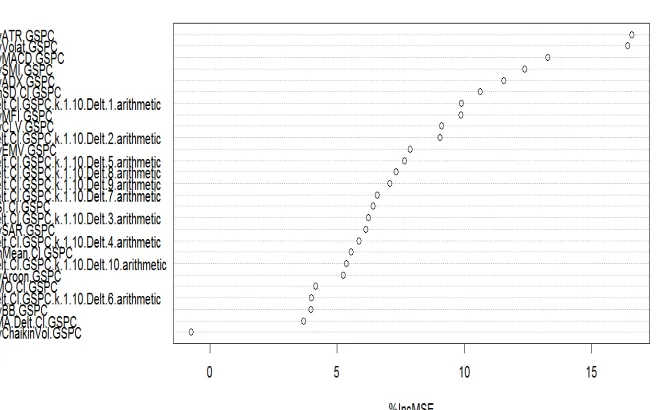
There are some representative set of technical indicators, from those available in package TTR—namely, the Average True Range (ATR), which is an indicator of the volatility of the series; the Stochastic Momentum Index (SMI), which is a momentum indicator; the Welles Wilder’s Directional Movement Index (ADX); the Aroon indicator that tries to identify starting trends; the Bollinger Bands that compare the volatility over a period of time; the Chaikin Volatility; the Close Location Value(CLV) that relates the session Close to its trading range; the Arms’ Ease of Movement Value (EMV); the MACD oscillator; the Money Flow Index (MFI); the Parabolic Stop-and-Reverse; and the Volatility indicator. we have carried out some post-processing of the output of the TTR functions to obtain a single value for each one. In our approach to this application, we will split the available data into two separate sets: (1) one used for constructing the trading system; and (2) other to test it. The first set will be formed by the first 30 years of quotes of S&P 500. We will leave the remaining data (around 9 years) for the final test of our trading system. By means randomforest of checking the importance of the variables(figure 2.1 Variable importance according to the random forest), we can decide on a threshold on the importance score to select only a subset of the features. Look at the figure 2.1 and given that this is a simple illustration of the concept of using random forests for selecting features, we will use the value of 9.5 as the threshold and choose eight technical indicators as follows, and the codes are behind the eight indicators.
[1] “Delt.Cl.GSPC.k.1.10.Delt.1.arithmetic” [2] “myATR.GSPC”
[3] “mySMI.GSPC” [4] “myADX.GSPC” [5] “myVolat.GSPC” [6] “myMACD.GSPC” [7] “myMFI.GSPC” [8] “runSD.Cl.GSPC”
The codes are:
>varImpPlot([email protected], type=1) >imp<-importance([email protected], type=1) >rownames(imp)[which(imp>9.5)]
63
Figure 2.1: Variable importance according to the random forest
2.4. Built the model
We built the model use the eight technical indicators. In R, the codes of ANN model for stock time series data are:
>set.seed(1234)
>norm.data<-scale(Tdata.train)
>nn<-+nnet(Tform,norm.data[1:1000,],size=10, +decay=0.01,maxit=1000,linout=T,trace=F) >norm.preds<-predict(nn,norm.data[1001:2000,]) >preds<-unscale(norm.preds,norm.data)
>sigs.nn<-trading.signals(preds,0.1,-0.1)
>true.sigs<-+trading.signals(Tdata.train[1001:2000,"T.ind.GSPC"],0.1,-0.1) >sigs.PR(sigs.nn,true.sigs)
The same as ANN, we built SVM model.
2.5. Model evaluation and selection based on window mechanism
64
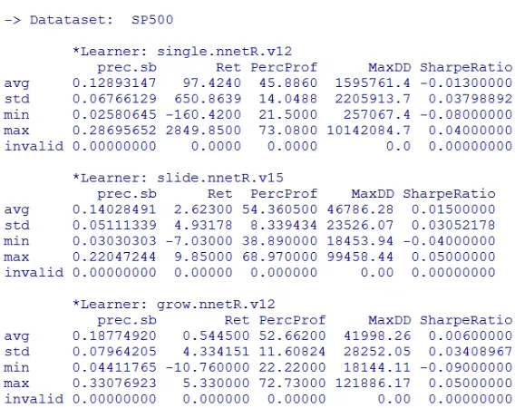
Use the function rankSystems(which is provided by R package:DMwR) we can obtain a top chart for the evaluation statistics in which we are interested, indicating the best models. The top five performance index are:$SP500$prec.sb, $SP500$Ret, $SP500$PercProf, $SP500$MaxDD, $SP500$SharpeRatio. And almost all these variants use some windowing mechanism. This provides some evidence of the advantages of these alternatives over the single model approaches, which can be regarded as a confirmation of regime change effects on these data. We can also observe several remarkable scores, namely in terms of the precision of the buy/sell signals.
Figure 2.2: Summary of Experiment Results
In order to reach some conclusions on the value of all these variants, we need to add some constraints on some of the statistics. Let us assume the following minimal values: we want (1) a reasonable number of average trades, say more than 20; (2) an average return that should at least be greater than 0.5% (given the generally low scores of these systems); (3) and also a percentage of profitable trades higher than 40%. The output of the experiment is figure 2.2:
As we can see, only three of the 120 trading variants that were compared satisfy these minimal constraints. All of them use a regression task and all are based on neural networks.
3. Conclusion and future work
65
window. From the result of experiment, we can make a conclusion that the favorite three models all use one of three models, and ANN is more suitable for stock time series data. The next work we will make a trading system to check the precision of this method.
Acknowledgments
This work is supported by the Fundamental Research Funds for the Central Universities 2014 (no.31920140089) and the National Natural Science Foundation of China (no.11161041).
REFERENCES
1. Qinghua Wen, Zehong Yang, Yixu Song, Perfa Jia, Automatic stock decision support system based on box theory and SVM algorithm, Expert Systems with
Applications, 37(2) (2010) 1015-1022.
2. Karin Kandananond, Applying 2k factorial design to assess the performance of ann and svm methods for forecasting stationary and non-stationary time series, Procedia
Computer Science, 22 (2013) 60-69.
3. Yanchang Zhao. R and Data Mining: Examples and Case Studies. ISBN 978-0-12-396963-7, December 2012. Academic Press, Elsevier. 256 pages. URL: http://www.rdatamining.com/docs/RDataMining.pdf.
4. Lin, X., Yang, Z., Song, Y., Washio T., et al. (2008). The application of echo state network in stock data mining. In PAKDD 2008: Vol. 5012. LNAI (pp. 932–937). 5. Marko Debeljak, Aleš Poljanec, Bernard Ženko,Modelling forest growing stock from