Semantic Image Interpretation

(1)

DEPARTMENT OF INFORMATION ENGINEERING AND COMPUTER SCIENCE ICT International Doctoral School

Integration of Numerical Data and Logical

Knowledge for Cognitive Vision

Ivan Donadello

Advisor

Luciano Serafini

Fondazione Bruno Kessler

Committee

Prof. Dr.

Marco Cristani

Universit`

a degli Studi di Verona

Prof. Dr.

Claudia d’Amato

Universit`

a degli Studi di Bari

Prof. Dr.

Tillman Weyde

City, University of London

Dr.

Daniele Porello

Libera Universit`

a di Bolzano

(2)

(3)

(4)

(5)

Abstract

Semantic Image Interpretation (SII) is the process of generating a structured description of the content of an input image. This description is encoded as a labelled direct graph where nodes correspond to objects in the image and edges to semantic relations between objects. Such a detailed structure allows a more accurate searching and retrieval of im-ages. In this thesis, we propose two well-founded methods for SII. Both methods exploit background knowledge, in the form of logical constraints of a knowledge base, about the domain of the images. The first method formalizes the SII as the extraction of a partial model of a knowledge base. Partial models are built with a clustering and reasoning algo-rithm that considers both low-level and semantic features of images. The second method uses the framework Logic Tensor Networks to build the labelled direct graph of an im-age. This framework is able to learn from data in presence of the logical constraints of the knowledge base. Therefore, the graph construction is performed by predicting the la-bels of the nodes and the relations according to the logical constraints and the features of the objects in the image. These methods improve the state-of-the-art by introducing two well-founded methodologies that integrate low-level and semantic features of images with logical knowledge. Indeed, other methods, do not deal with low-level features or use only statistical knowledge coming from training sets or corpora. Moreover, the second

method overcomes the performance of the state-of-the-art on the standard task of visual relationship detection.

Keywords

(6)

(7)

Acknowledgments

First and foremost, I want to thank my Ph.D. advisor Luciano Serafini, who has shown me and helped me to appreciate and adopt the mindset, the rigour and the commitment required for conducting quality research. By constantly working with him, I had the opportunity to learn many of the skills expected from a researcher.

Another important person for my Ph.D. is Artur d’Avila Garcez, who hosted and su-pervised me in the Research Centre for Machine Learning at City, University of London, during my visiting. I improved my research skills and acquired more knowledge about Machine Learning, and, more specifically in learning with logical constraints. The inter-action with Artur d’Avila Garcez brought very important (and published) results for my Ph.D.

Silvana Badaloni was my supervisor during the Master Thesis. I want to thank her for introducing me Luciano Serafini and for giving me the opportunity to spread my research as invited speaker at the University of Padova.

During my Ph.D., I had interactions with other people whose suggestions and interac-tions fruitfully impacted my work. Francesco Corcoglioniti and Marco Rospocher were my first guides to the topic of Semantic Web. The former taught me many tricks, best prac-tices and technicalities on Semantic Web programming. The latter was determinant for understanding ontologies and their management. The Laboratory for Applied Ontology (headed by Nicola Guarino) was important for the discussions about the ontological re-search part of my Ph.D. The discussions with Andrea Passerini and Stefano Teso brought a significant improvement of my knowledge on Machine Learning and optimization with logical constraints. They gave me important suggestions on both theoretical and technical aspects. I thank Enver Sangineto and Gloria Zen for their nice (and deep) introduction to the world of object detection.

(8)

For their feedback, technical advices, and support in any form, I want to thank my colleagues and friends (in alphabetical order): Greta Adamo, Loris Bozzato, Gaetano Calabrese, Elena Cardillo, Alessandro Daniele, Riccardo De Masellis, Mario De Nisi, Chiara Di Francescomarino, Shahi Dost, Mauro Dragoni, Marco Fossati, Chiara Ghidini, Radim Nedbal, Giulio Petrucci, Williams Rizzi, Andrea Rubin, Emilio San Filippo and Roberto Tiella.

(9)

List of Tables

4.1 SROIQ constructors . . . 25

4.2 SROIQ axioms . . . 26

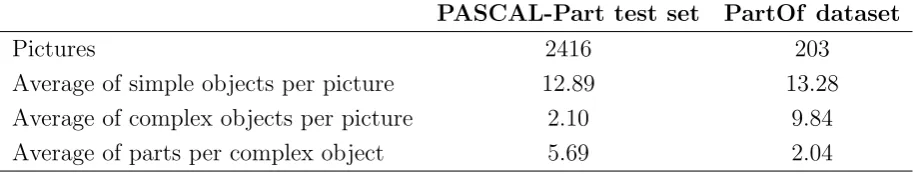
5.1 The PASCAL-Part and the PartOfdataset statistics . . . 45

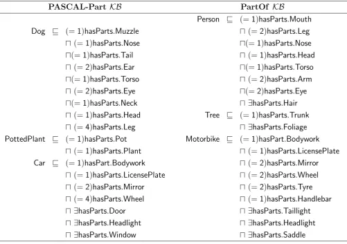
5.2 Excerpts of PASCAL-Part and PartOf knowledge bases . . . 46

5.3 The PASCAL-Part and the PartOfknowledge bases statistics . . . 46

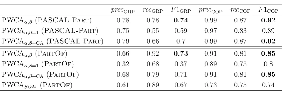
5.4 Results of the partial models evaluation . . . 49

8.1 The SII tasks for every considered dataset. . . 84

8.2 Visual Relationship Dataset statistics . . . 93

8.3 Results on the Visual Relationship Dataset . . . 97

(14)

(15)

List of Figures

2.1 Input of a SII system . . . 10

2.2 A semantically interpreted picture: the output of SII . . . 12

4.1 The relation between world, partial view, model and partial model . . . 28

4.2 Comparison between original and candidate partial models . . . 30

5.1 A hierarchical clustering dendogram . . . 35

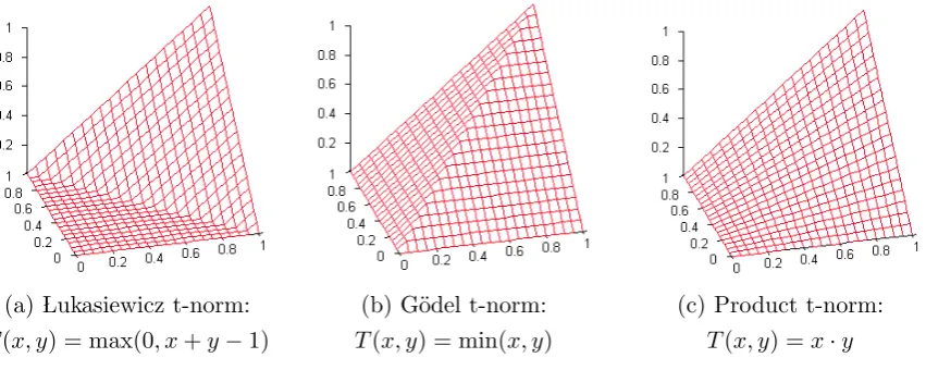
6.1 Examples of Fuzzy Logic t-norms . . . 56

6.2 Examples of Fuzzy Logic residua . . . 57

6.3 Examples of Fuzzy Logic t-conorms . . . 58

6.4 Example of Neural Tensor Network . . . 61

6.5 The angle between two bounding boxes . . . 65

6.6 Example of a Logic Tensor Network . . . 69

8.1 Results for indoor objects classification and the partOf relation . . . 88

8.2 Results for noisy training label experiments . . . 90

8.3 Visual relationship detection tasks . . . 92

8.4 Visual Relationship Dataset examples . . . 92

8.5 Long-tail aspect of the Visual Relationship Dataset . . . 93

A.1 KnowPic: initial page . . . 122

A.2 KnowPic: show picture page . . . 123

A.3 KnowPic: SII for a countryside scene . . . 124

A.4 KnowPic: SII for an indoor scene . . . 125

(16)

(17)

Chapter 1

Introduction

(18)

scene and where they are. Examples of this kind of analysis are: (i) the object detection that localizes objects within bounding boxes (a rectangle around the object); (ii) the semantic segmentation that associates every pixel a set of labels describing the object which the pixel belongs to. At this level of analysis, for example, it is possible to have the labels “countryside” and “green” that describe the whole image plus two bounding boxes classified with “person” and “horse”, respectively. However, to achieve a complete understanding of the scene, it is also necessary to discover some relations between the objects. In a third level of analysis of the image content, a detailed labelling of the objects in the scene, with their attributes, and the relations between them is performed. At this level, some background knowledge is of great help as it allows for reasoning about the visual objects in the scene. This reasoning improves the results of the analysis. For example, if the image analysis discovers that a person rides a horse then it is possible to infer that the contrary is false (the relation ride is antisymmetric). We can also infer that there are some animals in the image (horses are animals), that the person is on the horse, the horse is under the person and is carrying him/her. At this level, the analysis of the image content is very detailed and it is possible to organize the discovered objects, attributes and relations within a structure. For example, the objects (and attributes) can be nodes of a graph and the relations between objects can be the edges between the corresponding nodes. A fourth level of analysis performs some high-level reasoning on the image objects and relations to infer what is happening in the scene, that is, what are the main events and the participants. This level refines the previous level by extracting higher-level information from the structured description of the image content. For example, the graph returned by the third level could contain only the relation “on” between a person and a horse. Hence, the fourth level predicts the event “riding” as the most plausible event with the person and the horse as participants. This prediction can be encoded in the graph by adding, for example, a node labelled with “riding event” with two edges joining the person and horse nodes. These edges are labelled with the roles of the participants at the event, for example the subject and object of the event. The Semantic Image Interpretation (SII) [51, 71] is the task of extracting such a detailed structure of the image content.

The SII enables a set of applications on an image content that a coarse image descrip-tion (such that the one of the first layer) does not allow. Here we list some examples: Accurate Image Retrieval A structured description of an image content that links the

(19)

CHAPTER 1. INTRODUCTION

in their hand shot during a riot.

Complex Image Querying A structured image description can be easily converted into a RDF graph [41]. This allows us to perform structured queries on images by using Semantic Web languages, such as SPARQL [30]. These queries can have a certain complexity, for example they can be the join of two simpler queries: we want to retrieve all (and only) the images showing a person riding a horseand in the middle of some buildings.

Robot Interaction A robot moving in an environment can find many configurations of objects and these objects enable the robot to perform a set of actions on them. For example, a cup on a table can be grasped but without hitting the table.

Visual Question Answering Such a structured image description can be inspected in order to answer natural language questions about the image content. For example, a question could be “Is there anyone riding an animal?”, with answer “Yes, a person” and the involved bounding boxes.

Image/Video Captioning A structured description of an image can be easily converted (with a language generator model) into a natural language caption. This can be applied also to videos as they are a sequence of images (the frames).

The aim of this thesis is to study new algorithms and techniques in order to give an important contribution to the SII problem. However, the semantic interpretation of images presents some aspects that make the problem challenging:

Relational Domain The domain of images is relational, that is, the data (the labelled bounding boxes) are linked together through relations. For example, the pair of bounding boxes containing a person and a horse can be related through many predicates: (person, ride, horse), (person, on, horse), (horse, under, person) and (horse, carry, person).

(20)

Background Knowledge This domain can be described with some background knowl-edge about the input image. When a SII system analyses a picture, some important knowledge can be taken into account. For example, the fact that usually horses are ridden by people and horses do not ride. Moreover, background knowledge can impose constraints (such as, implication or mutual negation) between predicates: if a person rides a horse then the person is on the horse and, automatically, it cannot be under the horse.

1.1

Contributions

In this thesis we present two well-founded methods, with relative evaluation, to solve the SII problem. The first method extracts the structured description of an image content by combining an unsupervised algorithm with standard logical reasoning on the back-ground knowledge. The second method learns and predicts this structured description in a supervised manner. The background knowledge imposes logical constraints on such predictions. The contributions of these methods involve the following SII aspects:

C1 Integration of Numeric and Symbolic Features Both methods deal with the numeric features coming from a low-level analysis of images and the semantic fea-tures used to describe the image content.

C2 Dealing with Uncertainty The low-level analysis of images returns data with un-certainty. For example, an object detector could not be sure about the classification of some objects in the image. Both methods address the uncertainty of the data. C3 Integration of Logical Background Knowledge Both methods exploit background

knowledge that can be found, encoded as logical constraints, in knowledge bases. Logical knowledge is very powerful as it expresses, with a standard logical language, many information and constraints about the domain of the images.

(21)

(logical-CHAPTER 1. INTRODUCTION 1.2. STRUCTURE OF THE THESIS

based approaches) hardly deal with the uncertainty coming from a low-level analysis of the image.

1.2

Structure of the Thesis

The remainder of the thesis is structured as follows:

Chapter 2 This chapter provides the definition of the problem.

Chapter 3 This chapter provides the state-of-the-art on SII ranging from works on object detection to works on the construction of the graph that describes the image content. The background notions necessary to understand the thesis are not explained here but at the beginning of every chapter.

Chapter 4 This chapter provides a theoretical framework for SII that is used for imple-menting the first SII algorithm of the thesis. This chapter represents Contributions C3.

Chapter 5 This chapter provides the first (unsupervised) algorithm that mixes low-level and semantic features for SII. The chapter also describes the datasets used for the evaluation, the exploited knowledge bases, and finally the evaluation. This chapter represents Contributions C1, C2, C3.

Chapter 6 This chapter presents Logic Tensor Networks. This is a new framework that learns from data in presence of logical constraints. This chapter represents Contributions C1, C2, C3.

Chapter 7 This chapter provides how the SII problem has been encoded with Logic Tensor Networks. It also discusses some technical aspects of Logic Tensor Networks that emerge on the application to SII. This chapter represents Contributions C1, C2, C3.

Chapter 8 This chapter provides the evaluation of Logic Tensor Networks to SII. The chapter describes in details the considered datasets (and their statistics) and knowl-edge bases, the performed experiments, the obtained results along with a comparison with methods of the state-of-the-art. This chapter represents Contributions C1, C2, C3.

(22)

Chapter 10 This chapter provides a discussion of the presented algorithms. It summa-rizes the results of the thesis, discusses limitations and possible research directions. Appendix A This appendix describes a demo that implements a SII system according to the algorithms developed in the thesis. Some screenshots are provided to show the output of the system.

1.3

Publications

The core publications supporting the present thesis are listed below:

• Ivan Donadello, Luciano Serafini, and Artur S. d’Avila Garcez. Logic tensor net-works for semantic image interpretation. In Carles Sierra, editor, Proceedings of the Twenty-Sixth International Joint Conference on Artificial Intelligence, IJCAI 2017, Melbourne, Australia, August 19-25, 2017, pages 1596–1602. ijcai.org, 2017

• Luciano Serafini, Ivan Donadello, and Artur S. d’Avila Garcez. Learning and reason-ing in logic tensor networks: theory and application to semantic image interpretation. In Ahmed Seffah, Birgit Penzenstadler, Carina Alves, and Xin Peng, editors, Pro-ceedings of the Symposium on Applied Computing, SAC 2017, Marrakech, Morocco, April 3-7, 2017, pages 125–130. ACM, 2017

• Ivan Donadello and Luciano Serafini. Integration of numeric and symbolic informa-tion for semantic image interpretainforma-tion. Intelligenza Artificiale, 10(1):33–47, 2016

• Ivan Donadello. Ontology based semantic image interpretation. In Elena Bellodi and Alessio Bonfietti, editors, Proceedings of the Doctoral Consortium (DC) co-located with the 14th Conference of the Italian Association for Artificial Intelligence (AI*IA 2015), Ferrara, Italy, September 23-24, 2015., volume 1485 of CEUR Workshop Proceedings, pages 19–24. CEUR-WS.org, 2015

(23)

CHAPTER 1. INTRODUCTION 1.4. ARTEFACTS

1.4

Artefacts

The core artefacts supporting the present thesis are listed below (in ascending order of publications):

A1 The knowledge bases and the datasets for the experiments in [27]: https://dkm. fbk.eu/technologies/knowpic.

A2 The source code for the paper in [92]: https://gitlab.fbk.eu/donadello/LTN_ ACM_SAC17/.

A3 The source code for the paper in [28]: https://gitlab.fbk.eu/donadello/LTN_ IJCAI17.

(24)

(25)

Chapter 2

The Problem

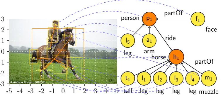
Semantic Image Interpretation (SII) is the task of generating a structured description of the content of images [51, 71, 55]. SII is much more than image classification [56], that is, the description of image content with a set of labels, SII aims at detecting the objects in images, their types, attributes and the relations between them. SII produces a semantically rich structure (for example, a logical model of a logical theory) that is both human understandable and processable by machines. Before defining the properties of such a structure we define what is the input of a SII system. As inputs we consider a background knowledge and asemantically labelled picture. To better explain our proposal, we use the simple running example of Figure 2.1.

(26)

Open Data. Examples of available logical knowledge are WordNet [34], YAGO [66], ConceptNet [100], Cyc [59] and DBpedia [3].

-5 -4 -3 -2 -1 0 1 2 3 4 5 -3 -2 -1 0 1 2 3 Tail

Leg Leg Leg Leg Muzzle

Leg Face

Arm

Horse

Person v (=1)hasParts.Face

u(=2)hasParts.Leg

u(=2)hasParts.Arm Horse v (=1)hasParts.Muzzle

u(=4)hasParts.Leg

u(=1)hasParts.Tail Horse v ∀hasPart.(¬Face)

u ∀hasPart.(¬Arm)

Person v ∀hasPart.(¬Muzzle) u ∀hasPart.(¬Tail)

Horse v ∀ride.⊥

Person v ∀ride−.⊥

Leg v Limb Arm v Limb

Figure 2.1: A semantically labelled picture and a Description Logic knowledge base that encodes the background knowledge.

(27)

CHAPTER 2. THE PROBLEM

Definition 1 (Semantically Labelled Picture). Let S ={s1, . . . , sn} be a set of segments

(a segment is a set of contiguous pixels) returned by a low-level analysis of picture P, and let Σ the signature of a logical language. A semantically labelled picture is a pair

P =hS, Li, whereLis a function that associates each segments∈Sa setL(s)⊆Σ×(0,1] of weighted labels hl, wi.

In this thesis we adopt the object detection as low-level technique of analysis of the input image because it is pretty forward to extract proposals for the objects. The labels associated to the bounding boxes are taken from the signature Σ used to specify the background knowledge. The semantically labelled picture of Figure 2.1 contains bounding boxes for the main objects in the image but some are missing. For example, there is no bounding box containing the whole person, neither for the grass, the sky and the trees in background. Notice that, if we search, at this stage, for a picture containing a person that is riding a horse, the picture will not be returned. The goal of SII is to build a semantic structure that contains also the presence of the non-recognized person and the fact that he is riding the recognized horse.

Given an input image, we define the structured description of the image content as a labelled direct graph with nodes and edges. A labelled node corresponds to segments of the input image containing an object. The labels of the node describe the corresponding object in the image: they can be attributes of the object (for example, “brown”) or clas-sification labels (for example, “horse”). A labelled direct edge starts from a subject node, ends in a object node and its labels (for example, “ride”) describe a relation between the corresponding objects in the image. This graph is also calledscene graph [55]. Moreover, nodes of the graph need to be aligned (that is, linked with) with the segments in the input image. That is, for every node of the graph, a SII system has to return the corresponding pixels in the image. This is necessary for the accurate image retrieval and visual question answering tasks mentioned in the previous chapter. We call this data structure seman-tically interpreted picture. Figure 2.2 shows the semanseman-tically interpreted picture of the running example.

(28)

we left the detection of some objects and and their properties (for example, the shape, the material or the texture) to robust Computer Vision techniques, such as the object detection, that learn the semantics of some objects and their properties. Whereas the information contained in the knowledge base is used to discover relations between objects or to refine the output of the Computer Vision analysis. For example, the knowledge base could correct a detected pois texture on a horse.

-5 -4 -3 -2 -1 0 1 2 3 4 5 -3 -2 -1 0 1 2 3 Tail Leg Leg Leg Leg Muzzle Leg Face Arm Horse p1

person _f₁

face a1 arm l5 leg partOf h1 horse t1 tail l1 leg l2 leg l3 leg l4 leg m1 muzzle ride partOf

Figure 2.2: A semantically interpreted picture: the output of SII. The labels inside the nodes are identifiers.

The main challenge in developing a system for SII for building a semantically inter-preted picture is bridging the so called semantic gap [51], which is the lack of a direct correspondence between the low-level features of an image and the high-level semantic concepts that a user adopts to interpret the picture. To address this problem the follow-ing research questions need to be posed:

1. what is an effective encoding for dealing with both low-level and semantic features of the image?

2. How can a SII system change (or discard) the proposals of an object detector if they disagree with other proposals?

3. How can a SII system infer the presence of some objects (or relations) with only few information coming from a low-level image analysis?

(29)

Chapter 3

State of the Art

The previous chapter defines the Semantic Image Interpretation as the procedure of con-structing a labelled graph, also called semantically interpreted picture or scene graph [55], that describes the semantic content of an input image. The labelled nodes represent ob-jects in the image, the labelled edges represent semantic relations between obob-jects. This review lists the main works that construct such a graph. These works are between two Ar-tificial Intelligence communities: the Computer Vision and the Knowledge Representation community. These works can be divided into three groups:

Object Detection This group does not properly contain SII works but the main ap-proaches necessary for extracting the basic components of a SII labelled graph: the nodes, that is, the objects in the image.

Visual Relationship Detection This group lists important works that build a labelled SII graph by predicting a set of visual relationships. A visual relationship is a relation between two objects in the image. In literature, a visual relationship is described as a triple hsubject, predicate, objecti where subject is the label of the node with an outgoing edge e, predicateis the label of the edge e and object is the label of the node receiving the edge e. If we refer to the running example of Figure 2.2, examples of visual relationships are: hPerson,ride,Horsei, hLeg,partOf,Personi

andhMuzzle,partOf,Horsei. The main idea underlying this set of works is to consider two nodes in the scene graph, and classify them according to a set of relationships. This approach performs a local choice by classifying, each time, the relationships between only two objects in the input image.

(30)

labelled node or edge) takes into account also the surrounding nodes, that is, the contextual information.

3.1

Object Detection

Object detection provides the labelled nodes of a scene graph. That is, the main objects that can be found in a picture. The literature on object detection is huge and a detailed review is out of the scope of this presentation. For this reason, we list the most relevant works. A first processing of object detection is given by the extraction of the object proposals. These are a set of non classified bounding boxes that may potentially contain an object. There is a huge literature on object proposal methods and comprehensive surveys can be found in [49, 14]. Most of the object proposal works can be divided in two groups: (i) those based on grouping super-pixels (for example, Selective Search [106], Constrained Parametric Min-Cuts (CPMC) [13], Multiscale Combinatorial Grouping (MCG) [76]) and (ii) those based on sliding windows (for example, objectness in windows [1], EdgeBoxes [115]). Object proposal methods can be adopted as image preprocessing tools for object detectors. These take the input proposals and classify (or discard) them with some labels [46, 114, 104, 45, 101, 21, 58, 36, 37].

(31)

CHAPTER 3. STATE OF THE ART 3.2. VISUAL RELATIONSHIP DETECTION

the bounding boxes. Other works are the so-called part-based models. They leverage the part-whole relation between whole objects and their parts to improve the object detection [17, 32, 35, 38, 32, 70]. We review some of them in the related work in Chapter 9.

3.2

Visual Relationship Detection

In [87] the notion of visual phrase is proposed as a prototype of visual relationship. The difference is that a visual phrase is associated to only a single bounding box that contains both subject and object. The work shows that the detection of visual phrases improves the detection of the single subjects and objects. The approach is based on training an object detector for every possible triple hsubject, predicate, objecti. This suffers of scalability issues as the number of categories for the subjects/objects and the predicates grows. Closely related to the visual relationship detection is the visual semantic role labelling [42, 85, 108]. This task extracts from pictures a set of tuples such as:

hpredicate,{hrole1, label1i, . . . ,hroleN, labelNi}i, where the roles represent some entities

involved by the predicate such as agent, source, tool or place. A visual relationship is a tuple with only the subject and the object as roles. In [42] the authors propose a dataset and baselines based on object detection and regression of bounding boxes of roles involved in a predicate. The roles are limited to subject (performing the action), object and instrument/tool. A limitation is that the role of subject is assigned only to people.

Many works exploit deep learning techniques [88] for visual relationship detection. For example, in [24] the visual relationships are detected with a novel (and designed specifically) Deep Relational Network that exploits the statistical dependencies between relationships and the involved objects. In [61] the use of a deep reinforcement learning framework to detect visual relationships and attributes of objects is exploited. The au-thors of [60] propose a message passing algorithm to share information (and reasoning) among neural networks that encode the subject, the object and the predicate of a visual relationship. In [112] the visual relationship detection is related to the similarity of the subject and object in the same vector space. Indeed, the difference between the embed-ding vectors of the subject and the object gives information on the relationship between them.

(32)

a visual relationship is predicted with a score that combines the background knowledge with the visual information. The former is a pre-trained word embedding (word2vec) [67] of the subject and object labels, such that similar triples are close in the embedding space. The latter consists in the visual features of the union of the subject and object bounding boxes (computed with a CNN). The work in [6] combines background knowledge with visual information in the same manner of [65]. The difference is that the considered knowledge is statistical information about the triples in the training set. For example, the likelihood that a wheel is part of a car. This knowledge is learnt with statistical link prediction methods [72]. In [109] the background knowledge (taken from the training set and Wikipedia documents) is encoded as a probability distribution of a relationship given the labels of the subject and the object. During the training phase, this knowledge drives the learning of a fully connected neural network that predicts visual relationships. Other approaches encode background knowledge with visual features in probabilistic graphical models. In [113, 73], visual features are combined with knowledge gathered from datasets, web resources or annotators, about object labels, properties (for example, shape, colour, size) and affordances, using a Markov Logic Network (MLN) [84]. This allows for querying of the MLN and thus to predict visual relationships in unseen images. Due to the specific knowledge-base schema adopted, the effectiveness of MLNs in this domain is evaluated only for Horn clauses, although the language of MLNs is more general.

3.3

Direct Graph Construction

Several works build a semantically interpreted picture by considering its labelled graph as a whole and not only its single components (the visual relationships). Indeed, the surrounding context can help the recognition of both objects and relations between them. For example, suppose we have bounding boxes for a horse, grass and a person (this last one with a low score). The presence of a horse and grass increases the likelihood to have a person that rides (or walks with) the horse that is on the grass. The first works that follow this intuition come from the Knowledge Representation community and they formalize the labelled graph of the SII as an interpretation of a logical language. Indeed, the scene graph is a set of logical statements in a logical language, for example, Horse(h1),

Person(p1), ride(p1,h1). The scene graph is built with logical reasoning. The first work

(33)

CHAPTER 3. STATE OF THE ART 3.3. DIRECT GRAPH CONSTRUCTION

description of the image content is derived. However, such a complete description cannot be obtained for a picture. In [89] the picture is represented with the notion ofpartial model of a knowledge base. The generation of a semantically interpreted picture is performed with pure logical reasoning but low-level features of the image are not considered. In [71] the low-level image features are included in a Description Logic (DL) [5] knowledge base along with DL axioms. These axioms represent the connection between semantic types and low-level features (via data properties and concrete domains). For example, the standard dimension of a plate is formalized with a constraint on the data property

size of the concept of plate. The graph construction is derived via deductive reasoning and a notion ofpreference between partial models is considered. However, writing axioms that map low-level features in concepts and relations could suffer of scalability (high engineering effort) as the number of concepts and relations grows and dealing with the noise coming from object detectors could be problematic. A different approach to the scene graph construction is based on abductive reasoning [74]. This technique infers the preferred partial model (explanation) starting from the observations coming from a low-level image processing (object and spatial relation detection). The preferred partial model of an image is the one that contains more evidence and less hypotheses. However, the method requires a set of DL rules for defining the abducible space, which need to be manually crafted. Other logic-based approaches use fuzzy DL to deal with the uncertainty coming from the object detection [50, 2]. These approaches limit themselves to spatial relations or to refine the labels of the detected objects. In [50] the authors proposed a fuzzy DL ontology of spatial relations and an algorithm for building scene graphs. The scene graph is constructed starting from some basic objects in the scene, then, through logical reasoning, semantic relations between objects (or new objects) are inferred. This method is extended in [2] where morphological reasoning [29] is applied to the objects discovered by the low-level image analysis.

(34)

(35)

Chapter 4

Semantic Image Interpretation as a

Ranking of Partial Models

In this chapter, a formal, and logic-based framework for Semantic Image Interpretation (SII) is described. The first observation is that an image is a partial view of the world. That is, the scene in a image can be cluttered and some objects cannot be visible or satisfy our background knowledge. For example, due to occlusions we can see only one leg of a person riding a horse. However, we are able to reason about this partial view, find an explanation to the lack of the other leg of the person and deduce that the partial view satisfies our background knowledge. With this intuition we formalize a semantically interpreted picture as a partial model of an input knowledge base, see Figure 2.2, that is, a logical interpretation whose completion satisfies the knowledge base. Moreover, many partial models exist for an input image, thus there is the need to find the one that best matches the image content. This is formalized with a cost function that assigns a cost to partial models. This function measures the (dis)agreement between the low-level features of our input image and the high-level semantic features contained in the partial model. Therefore, a semantically interpreted picture is a partial model that minimizes a cost function. As input, we assume to have a semantically labelled picture and a Description Logic knowledge base. The single segments of the input picture are labelled with the symbols in the signature Σ of the knowledge base, see Definition 1 and Figure 2.1.

(36)

4.1

An Overview of Description Logics

Description Logics (DLs) [5] are one of the main formalisms for knowledge representa-tion. DL languages have been widely used, from the middle of the ’80s, for knowledge representation [5] and ontology engineering [39]. Moreover, they are an important under-pinning for the OWL web ontology language as the World Wide Web Consortium (W3C) standardized.

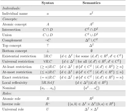
DLs stemmed from early days of knowledge representation formalisms (late ’70s, early ’80s) such as semantic networks and frame-based systems. The former are graph-based formalisms for representing the meaning of sentences. The latter are data structures used to divide knowledge into substructures by representing “stereotyped situations”. They can be considered as antecedents of object-oriented languages. Both are comprehensi-ble and intuitively readacomprehensi-ble but they lack of a formal semantics. DLs were developed to overcome these limitations by providing (i) a clear semantics and (ii) inference tech-niques. The DLs formal semantics provides an unambiguous meaning to sentences of the DL language and allows a common grounding for humans and interoperability be-tween humans and machines. Moreover, semantics makes possible to define a correct and complete logical deduction for inferring new information from facts of a knowledge base. This feature distinguishes DLs from other representation languages, such as the Unified Modelling Language (UML) [11] and the Entity-Relationship model language [16]. The process of computing inferences is called reasoning, and a computationally efficient rea-soning algorithm is an important feature of a DL. This is one of the reasons about the existence of many description logics: the higher the expressivity of the language the higher the computational cost for reasoning. The best balance between them depends on the application. In the following we describe: (i) the syntax (with basic modelling notions), (ii) the semantics of a particular, and highly expressive, DL: SROIQ [48], and (iii) a brief overview of reasoning in DLs.

4.1.1

Syntax of Description Logics

All DLs provide the basic building blocks for modelling entity types and relationships between entities in a domain of interest. We start with the notion of signature Σ = ΣI ]ΣC ]ΣR, or vocabulary, of a DL that is the set union of three finite and disjoint

sets of symbols: the individual names ΣI, the concept names ΣC and the role names

ΣR. Individual names represent single individuals of our domain whereas concept names

(37)

CHAPTER 4. SII AS MODELS RANKING 4.1. DESCRIPTION LOGIC

In the standard translation of DL in FOL [12] individual names correspond to constants, concepts correspond to unary predicates and roles to binary predicates. If we want to model the scene in a picture, for example the one in Figure 2.1, we use two individual names, john,furia ∈ ΣI, for representing the person and the horse, the concept names

Horse,Person ∈ ΣC to represent their types and the role name ride ∈ ΣR to represent

the relation of a person riding a horse. In this presentation, we focus on the syntax of one of the most expressive DLs: SROIQ[48]. Its high expressiveness is determinant for reasoning in a domain such as image interpretation. Indeed, in SII, some roles can be transitive (S) such as the roleright of. Some roles can include others (R), for example the role on includes the role ride. There can be the presence of nominals (O), for example a trained object detector could detect the presence of the individual Barack Obama. A role can be the inverse of another one (I), for example the roleright of is the inverse ofleft of. Finally, concept and role names can be related throughqualified number restrictions (Q), for example we know a priori that horses have exactly four legs. A SROIQ concept is an expression defined by the following grammar:

C, D := A| ¬C|CuD|CtD| > | ⊥ | ∃R.C | ∀R.C |

(≥n)R.C |(≤n)R.C | ∃R.Self | {a1, ..., an}

with A ∈ ΣC, R ∈ ΣR, and n is a non-negative integer. We assume that ΣR is closed

under inverse role, that is, ifR ∈ΣRthenR−(the inverse ofR, see Table 4.1) is in ΣR. In

addition, ΣRcontains also theuniversal role U that always relates all pairs of individuals.

We briefly describe the grammar:

• every concept name A∈ΣC is a concept expression;

• if C, D are concept expressions then also the negation ¬C is a concept expression. For example, the concept Male can be defined as ¬Female. The disjunction CuD

of two concepts is a concept expression. For example, the expression HorseuBrown

defines the concept of horses that have have brown fur. The conjunction CtD of two concepts is a concept expression. For example, the expression HorsetPerson

defines a concept (such as Animal in our picture domain) that includes people and horses.

• >(top concept) and⊥(bottom concept) are concept expressions. They are syntactic sugars for the concept expressions Ct ¬C and Cu ¬C, respectively.

• If R ∈ ΣR and C is a concept expression, then the existential quantification ∃R.C

(38)

entities with a tail. The universal quantification ∀R.C is also a concept expression. For example, the expression ∀eat.(GrasstVegetable) indicates all the entities that eat only grass or vegetables, such as horses.

• if R ∈ΣR,n is a non-negative integer and C is a concept expression, then ∃R.Self

(self restriction), (≥ n)R.C (at-least restriction), (≤ n)R.C (at-most restriction) and (= n)R.C (exact restriction) are also concept expressions. The latter three are also known as qualified number restrictions, or cardinality constraints, and impose a constraint on the cardinality of the quantifier. For example, the expression (= 4)hasPart.Legindicates all the entities with exactly four legs, that is the quadrupeds.

• {a1, ..., an}(nominal concepts) is a concept expression for every finite set{a1, ..., an} ⊆

ΣI of individual names, for example, {john,furia}.

As DLs are formal languages it is possible to create statements called axioms. The axioms state information about our domain and are collected into three sets: assertional axioms (ABox A), terminological axioms (TBox T) and relational axioms (RBox R). A DLs knowledge base KB is the union of these sets of axioms. ABox axioms encode factual knowledge about individuals, such as, the (negated) concept assertions:

Person(john),¬Horse(john),¬Person(furia),Horse(furia),

stating that the individual name john is an instance of the concept Person and not an instance of Horse. The individual name furia is an instance of Horse and not of Person. The (negated) role assertions describe relations between the individuals, such as, the individual john is riding the individual furia and not vice versa:

ride(john,furia),¬ride(furia,john).

ABox axioms state also the equality or not between individual names. This is necessary due to the fact that in DL a single individual of the domain can be represented by many individual names. For example, the individual inequality assertionjulia6≈johnstates that Julia and John are different individuals, whereas theindividual equalityassertionjohnny ≈ john states that Johnny and John are the same individual. On the other hand, the axioms in the TBox assert relationships between concepts, such as the concept inclusion. For example:

HorsevAnimal

states that all the individuals of type horse are also animals. The concept equivalence states that two concepts have the same individuals:

(39)

CHAPTER 4. SII AS MODELS RANKING 4.1. DESCRIPTION LOGIC

TBox axioms define concepts in terms of set theoretic combinations of other concepts, according to a specific DL syntax, see the grammar of SROIQ defined above. Finally, RBox axioms encode properties of roles such as therole inclusion. For example:

ridevon

states that every pair of individuals related with the ride role are also related with on. The role equivalence axiom states that two roles have the same pairs of individuals, for example above ≡ over. Another RBox axiom is the complex role inclusion that relates roles through their composition and inclusion. For example, it is possible to concatenate the carry and hasPart roles to state that every time a subject carries an object then the subject carries also the parts of the object:

carry◦hasPartvcarry

Finally, the role disjointness axioms state that two different roles cannot share pairs of individuals. For example, it is not possible that John is on and below the horse at the same time: Disjoint(on,below). The defined axioms can be resumed in the following table:

ABox axioms TBox axioms

C(a) concept assertions CvD concept inclusion

¬C(a) negated concept assertions C≡D concept equivalence

R(a, b) role assertions

¬R(a, b) negated role assertions

a≈b individual equality

a6≈b individual inequality

RBox axioms

RvS role inclusion

R≡S role equivalence

R◦SvQ complex role inclusion

Disjoint(R, S) role disjointness

4.1.2

Semantics of Description Logics

(40)

(true or false) of an axiom. An interpretation I of Σ is a pair h∆I,·I_i_{, where ∆}I _{is a}

non-empty set, called theinterpretation domain, that can be conceived as the collection of individuals, or things, that exist in the “world” that I represents. The function·I_{, called}

interpretation function, grounds the symbols in the signature Σ (individuals, concepts

and roles) in the elements of ∆I according to the following rules:

• individual names are interpreted as elements of the domain, formally ·I _{: Σ}

I →∆I;

• concept names are interpreted as subsets of the domain, formally ·I _{: Σ}

C →2∆

I

;

• role names are interpreted as binary relations, formally ·I _{: Σ}

R→2∆ I_×_∆I

;

An interpretation is a complete abstract description of the state of the world in terms of existing objects (that is, the elements of ∆I), object types (that is, the interpretations via ·I _{of the symbols in Σ}

C) and relations between objects (that is, the interpretations of

the symbols in ΣR). By now, the defined interpretation determines only the semantics of

the symbols in the signature Σ. However, to compute the truth value of a DLs axiom it is necessary to extend the interpretation function·I _{also to complex (}_SROIQ_{) concepts and}

roles. This extension is rather intuitive, for example the interpretation of HorseuBrown

(see above) is the intersection of the interpretation of HorseandBrown, see Table 4.1. We can now define the truth value (true or false) of an axiom according to an interpretation. An axiom φ issatisfied byI (or is true under I), in symbolsI |=φ, if the corresponding condition in Table 4.2 is met. If I satisfies all the axioms in a knowledge base KB, in symbols I |= KB, we say that I is a model for KB. We say that KB is consistent (or satisfiable) if it is satisfied by at least one model. An axiom φ is a logical consequence of

KB (or KB entails φ, in symbols KB |=φ) ifφ is true in every model of KB. The axioms of the knowledge base are constraints on the states of the world. For instance, the axiom

Horse v(= 4)hasPart.Leg states that every horse has exactly four legs. This implies that worlds where horses have only three or five legs are impossible.

4.1.3

Reasoning in Description Logics

Semantics provides a meaning to a KB symbols and defines what a logical consequence between axioms is, but it does not state how to compute (if possible) the entailments. This computation is called reasoning and one great advantage of DLs is that many reasoning tasks are decidable. We describe some important reasoning tasks:

(41)

CHAPTER 4. SII AS MODELS RANKING 4.1. DESCRIPTION LOGIC

Syntax Semantics

Individuals:

Individual name a aI

Concepts:

Atomic concept A AI

Intersection CuD CI∩DI

Union CtD CI∪DI

Complement ¬C ∆I \CI

Top concept > ∆I

Bottom concept ⊥ ∅

Existential restriction ∃R.C {d∈∆I |for some hd, d0_{i ∈}_RI_{, d}0 _∈_CI_}

Universal restriction ∀R.C {d∈∆I |for all hd, d0_{i ∈}_RI_{, d}0 _∈_CI_}

At-least restriction (≥n)R.C {d∈∆I |#{d0 _∈_CI _{| hd, d}0_{i ∈}_RI_{} ≥}_n}

At-most restriction (≤n)R.C {d∈∆I |#{d0 _∈_CI _{| hd, d}0_{i ∈}_RI_{} ≤}_n}

Exact restriction (=n)R.C {d∈∆I |#{d0 _∈_CI _{| hd, d}0_{i ∈}_RI_}₌_n}

Local reflexivity ∃R.Self {d∈∆I|hd, di ∈RI}

Nominal {a1. . . an} {aI. . . aIn}

Roles:

Atomic role R RI

Inverse role R− {ha, bi ∈∆I×∆I|hb, ai ∈RI}

Universal role U ∆I ×∆I

Table 4.1: Syntax and semantics of SROIQ constructors with a, b ∈ ΣI, A ∈ ΣC is a

concept name, C and D are concept expressions, R ∈ ΣR and #S is the cardinality of

(42)

Syntax Semantics ABox axioms:

Concept assertion C(a) aI ∈CI

Negated concept assertion ¬C(a) aI 6∈CI

Role assertion R(a, b) haI_{, b}I_{i ∈}_RI

Negated role assertion ¬R(a, b) haI_{, b}I_{i 6∈}_RI

Individual equality a≈b aI =bI

Individual inequality a6≈b aI 6=bI

TBox axioms:

Concept inclusion C vD CI ⊆DI

Concept equivalence C ≡D CI =DI

RBox axioms:

Role inclusion RvS RI ⊆SI

Role equivalence R≡S RI =SI

Complex role inclusion R1◦R2 vS RI1 ◦RI2 ⊆S

Role disjointness Disjoint(R, S) RI∩SI =∅

Table 4.2: Syntax and semantics ofSROIQaxioms witha, b∈ΣI,C andD are concept

(43)

CHAPTER 4. SII AS MODELS RANKING 4.2. PARTIAL MODELS RANKING

checks the existence (yes or not) of a model for KB. Checking knowledge bases consistency is very important as they model information of the real world that cannot be contradictory. Indeed, in most of the cases, contradictory axioms have no benefits and could be very dangerous, for example in applications for managing power plant systems. This reasoning task will be used in our first SII algorithm for checking the existence of a partial model describing a picture. Indeed, we want to discard interpretations that contradict the knowledge base axioms. For example, interpretations where horses have more than four legs.

Axiom Entailment A DL knowledge base KB entails an axiom φ if φ is true in every model ofKB. The reasoning task here is to check ifKB |=φor not. This task allows a user to “logically query” a knowledge base by checking if a new input axiom is true or not.

Concept Satisfiability A concept C ∈ ΣC is satisfiable, with respect to KB, if there

exists a model I of KB that maps C to a nonempty set: CI 6=∅. Concept satisfia-bility can be reduced to axiom entailment by checking whether KB |=C v ⊥, and thus it is a decision problem with yes or not as answer.

All these tasks are decidable in DLs and there exist sound and complete decision proce-dures to compute the reasoning. These proceproce-dures are implemented in optimized tools calledreasoners that are freely available, such as FaCT++ [105], HermiT [94], Pellet [96] and RacerPro [43]. The reasoning paradigm underlying these tools is the tableau method [5] that tries to construct models of a given knowledge base. If this succeeds, the knowl-edge base is satisfiable, if the construction necessarily fails then there is unsatisfiability.

4.2

Semantic Image Interpretation as a Partial

Mod-els Ranking

In this section we provide a formal (logic-based) framework for defining a semantically interpreted picture. The inputs of our framework are a semantically labelled picture P, that can be computed with an object detector (for example Fast R-CNN [36]) and a DL knowledge baseKB with signature Σ. The symbols in Σ are used as labels for the object detector.

(44)

KB. This view can be considered as an interpretation of the language of KB, but it does not necessarily satisfy all the axioms of KB. Indeed, the claim that a person has two legs is not satisfied in the picture but it is satisfied in the real world, supposing to be in a normal situation. Thus, if we formalize the world as a model of our knowledge base KB, we formalize the picture with the notion of partial model1 Ip of KB, see Figure 4.1.

Real World −−−−−−−−−−→formalized by ModelI of KB

partial view x  

x  ⊆

Picture −−−−−−−−−−→

formalized by Partial Model Ip of KB

Figure 4.1: The world is formalized with a model of KB and the partial view of the world contained in the picture is formalized with a partial model of KB.

Definition 2 (Extension of an Interpretation). Let I and I0 _{be two interpretations of the}

signatures Σ and Σ0 respectively, with Σ⊆Σ0; I0 _{is an} _{extension of} _I_{, or equivalently} _I0

extends I, in symbols I0 _{⊇ I}_,if _∆I _⊆_∆I0

, aI =aI0, CI =CI0∩∆I RI =RI0∩∆I×∆I, for all a∈ΣI, C ∈ΣC and R∈ΣR.

Definition 3 (Partial Model). Let KB a knowledge base, Ip is a partial model for KB,

in symbols Ip |=p KB, if there is a model I of KB (I |=KB) that extends Ip.

Following the intuition about partial models we define the semantic image interpreta-tion as the computainterpreta-tion of a partial model Ip =h∆Ip,·Ipiof KB. Thus, the construction

of a structured representation of the semantic content of an image consists in a method for creating the individuals (the nodes) of ∆Ip_{, assigning them a type and linking} to-gether (the edges) according to ·Ip_{. Having this graph describing the image content is} not enough. We need also the information about the object detection. For example, in an information retrieval system it could be also necessary to return the single bounding boxes. So, we need a link between the elements of our partial model and their corre-sponding bounding boxes. This consideration leads to the following formal definition of a semantically interpreted picture.

Definition 4 (Semantically Interpreted Picture). Given a knowledge baseKB with signa-ture Σ and a semantically labelled picture P =hS, Li, a semantically interpreted picture is a triple _S= (P,Ip,G) where:

(45)

CHAPTER 4. SII AS MODELS RANKING 4.2. PARTIAL MODELS RANKING

• Ip =h∆Ip,·Ipi is a partial model of KB;

• G ⊆∆Ip_×_S _{is a left-total}2 _{relation called} _{grounding relation.}

The grounding of every d∈∆Ip_{, denoted by} _G₍_d_{), is the set} _{s_∈_S _{| hd, si ∈ G}}_.

Figure 2.2 shows a semantically labelled picture that describes our running example. The partial model contains a person riding a horse with four legs, a muzzle and a tail, whereas the person has a visible leg, a visible arm and a face. The grounding of the parts and the horse are the corresponding initial bounding boxes, whereas the grounding of the person is the union of the bounding boxes associated to its parts. Note that the above definition can be stated also for the more expressive First-Order Logic. We focus on the

SROIQ DL [48] due to its high expressivity (see above) and its decidability. Indeed, the computation of a partial modelIp requires the use of a reasoning tool for checking if

Ip |=p KB (knowledge base satisfiability), see Section 4.1.3.

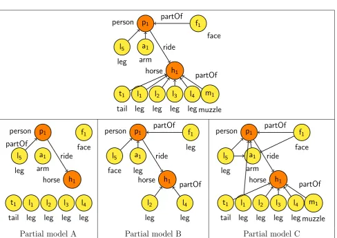
The picture content can be described by many partial models. Figure 4.2 shows the original partial model of our running example (above) and three partial models (below). That is, these partial models satisfy the constraints of KB in our running example (Fig-ure 2.1) but do not encode the real content of the pict(Fig-ure, they contain some errors or miss some information. Indeed, partial model A contains almost all the original nodes corresponding to objects but it misses many relations between objects. Partial model B contains correct relations but it misses many nodes and some nodes have wrong labels (the nodesa1,f1 andl5). Finally, partial model C contains all the nodes, many correct relations

but with additional errors (there is, for example, a partOf relation between a Leg and an

Arm). However, Definition 4 does not provide any criterion to select the partial model that better describes the content of a picture. We need a criterion to decide whether a partial model is a good explanation of the picture content. A criterion for the selection of a partial model could be the comparison with an original partial model of the picture, also known asground truth GT. A method of comparison is a function that returns a score S

(or costL) of similarity (or dissimilarity) between a partial model and the ground truth. This function enables us to rank the partial models and to return the best one, that is, the one that best matches the image content. Such a function can take into account the num-ber of correct labelled tripleshsubject node−relation−object nodeiin the partial model graph. For instance, the partial model A contains the tripleshperson p1−ride−horse h1i

and hleg l5 −partOf−person p1i. Examples of ranking functions consider the fraction

2_{Every logical individual is associated to at least one bounding box. A bounding box can have no}

(46)

p1

person f1

face a1 arm l5 leg partOf h1 horse t1 tail l1 leg l2 leg l3 leg l4 leg m1 muzzle ride partOf p1 person a1 arm l5 leg partOf f1 face h1 horse t1 tail l1 leg l2 leg l3 leg l4 leg ride p1

person f1

leg a1 leg l5 face partOf h1 horse l2 leg l4 leg partOf ride p1

person f1

face a1 arm l5 leg partOf h1 horse t1 tail l1 leg l2 leg l3 leg l4 leg m1 muzzle ride partOf

Partial model A Partial model B Partial model C

Figure 4.2: The original partial model of Figure 2.2 (above) and three partial models of the same input picture (below). For presentation purposes the edges without labels are implicitly labelled with partOf.

of correct triples in a partial model according to the ground truth GT or the fraction of retrieved triples of the GT. These functions are also known as precision and recall:

Sprec=

|partial model correct triples|

|partial model triples| , Srec =

|partial model correct triples| |correct GT triples| .

These functions consider different aspects of the partial models and thus return different rankings. If we consider Sprec, the ranking, with scores, is A (1.0), C (0.75), B (0.5). On

the other hand, the ranking with Srec is C (0.9), B (0.3), A (0.2). The difference in the

ranking position of partial model A is due to the fact that this partial model has only few but correct triples. We introduce a loss function LKB that measures the “distance”

between the partial model and the image content in order to perform a ranking of partial models and choosing the best one. The most plausible partial model I∗

(47)

CHAPTER 4. SII AS MODELS RANKING 4.2. PARTIAL MODELS RANKING

model that minimizes LKB:

(I∗

p,G

∗_{) = argmin} Ip|=pKB G⊆∆Ip×S

LKB(P,Ip,G). (4.1)

LKB measures the (dis)agreement between low-level image features of P and high-level

semantic features contained in Ip, with respect to the low-level/high-level mapping G.

The higher LKB(P,Ip,G) the less the agreement between Ip and P. For instance, if the

elementd∈∆Ip _ofI

p is grounded to the segment s(G(d) ={s}) then LKB is lower when Ip assigns todthe types that correspond to the labels ofswith higher weights. Similarly,

LKB penalizes the partial models that satisfyR(d, d0) when the low-level features of G(d)

andG(d0) are in disagreement with the relationR. For example,LKBpenalizes the models

that satisfyclose(d, d0) when the relative distance betweenG(d) andG(d0) is high. As can be seen from the above examples, the definition ofLKB heavily depends on the semantics

expressed byKB and on the picture content. Thus, a partial model is a good explanation of the picture content if it minimizes LKB. It is worth to notice that the number of

partial models can be huge according to the complexity of the image, that is, the number of segments of the input labelled picture. Therefore, it is infeasible to explore the whole search space of partial models in order to minimizeLKB. There is the need of algorithms

that find the pair (I∗

p,G

∗_{) in scalable manner. For example, in the next chapter, the}

proposed algorithm has polynomial time complexity according to the input image. Definition 5 (Semantic Image Interpretation Problem). Given a knowledge base KB, a semantically labelled pictureP and a loss functionLKB, the semantic image interpretation

problem is finding a partial model Ip and a grounding G that minimize LKB(P,Ip,G).

(48)

(49)

Chapter 5

Ranking Partial Models with

Clustering

In this chapter, a clustering technique for predicting the best partial model that describes an image content is developed. The idea is to start from already detected objects in the image and cluster them according to some relation. This intuition holds for many relations such as the part-whole relation or the relations that describe events. For example, for the part-whole relation whole objects and their parts need to be grouped together. Regarding the events, the objects participating at the event need to be clustered. Moreover, also the type of the whole object/event has to be discovered. The great advantage of clustering techniques relies in their unsupervision: there is no need of a ground truth of partial models as training set along with a training phase.

(50)

5.1

An Overview of Cluster Analysis

Cluster analysis [102] (or simplyclustering) divides input data (called data set) into groups (calledclusters) that are understandable by humans. This means that the clusters should capture the natural structure of the data, that is, the elements on the same cluster share similar features. Cluster analysis is a useful tool for data analysis, information extraction and as preprocessing technique for other types of analysis, such as data summarization or data compression. Cluster analysis has been applied in a wide variety of fields: psy-chology (for example, identification of different types of depression), biology (for example, the automatic creation of taxonomies or the understanding of gene functions), business analysis (for example, the segmentation of customers for marketing activities), pattern recognition (used, for example, in understanding the Earth’s climate), information re-trieval (for example, for grouping the results of a search engine query), machine learning, and data mining.

Clustering is the problem of grouping the elements of the data set into groups (clus-ters) so that the elements within a group are similar each other (intra-cluster similarity) and different from the elements in the other clusters (inter-cluster similarity). The greater the similarity within a cluster and the greater the difference between clusters, the better, or more separate, the clustering. A collection of clusters is commonly referred as a clus-tering. The are several types of clusterings, the main distinction is between partitional and hierarchical clustering. In partitional clustering the clusters are a partition of the data set: every object is assigned to one cluster and the clusters are pairwise disjoint. Hierarchical clustering is a generalisation of partitional clustering where clusters can be recursively clustered in higher-level clusters.

We briefly describe the following two clustering techniques as a background for under-standing our initial proposals to the Semantic Image Interpretation problem: the agglom-erative hierarchical clustering [102] and the Self-Organizing Maps clustering [53]. The former technique is suitable for exploring the huge search space of clusterings by repeat-edly aggregating clusters and evaluating a loss function on the result. The latter has been chosen as a sort of baseline for comparison due to its ability of automatically estimate the number of clusters, see next sections.

5.1.1

Agglomerative Hierarchical Clustering

The agglomerative hierarchical clustering [102] technique starts with N elements as indi-vidual clusters and, iteratively, merges the closest pair of clusters. This requires anN∗N

(51)

hier-CHAPTER 5. RANKING AS CLUSTERING 5.1. CLUSTERING

Algorithm 1: Basic Agglomerative Hierarchical Clustering Algorithm.

Input: A data set and a similarity matrix 1 Assign each item to a cluster.

2 repeat

3 Find the most similar pair of clusters in the similarity matrix and merge them together.

4 Update the similarity matrix to reflect the proximity between the new cluster and the

original clusters.

5 untilOnly one cluster remains.

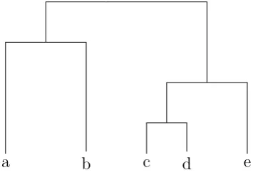
archical clustering can be graphically displayed as a tree-like diagram called dendrogram, see Figure 5.1, which displays both the cluster-subcluster relationships and the order in which the clusters were merged. A crucial operation of Algorithm 1 is the updating of

a b c d e

Figure 5.1: A hierarchical clustering of five elements shown as a dendrogram.

the similarity matrix between the new cluster and the original ones. This boils down to define a similarity between clusters, or groups of elements. Examples of common cluster similarities are the MIN, MAX and Group Average functions. The MIN function defines the similarity between two cluster as the similarity between the two closest points in the clusters. The MAX function is the opposite: it considers the similarity between the two farthest points in the clusters. Finally, the group average function defines the cluster similarity as the average pairwise similarity of all pairs of points with the first component in one cluster and the second component in the other cluster.

An important issue of hierarchical clustering regards the number of output clusters (or configuration). For example, the whole dendogram could be of little interest and a cut of the tree at a certain height could be more significant. If we consider the clustering of Figure 5.1 we can have the following clusterings (with a different number of clusters)

(52)

of the clusters such as the intra-cluster error sum Λ and the inter-cluster error sum Γ. We briefly describe the method proposed in [52] as a background of our clustering algorithm for SII described in Section 5.2.

Let D = {e1}Ni=1 a dataset of N elements where each element is a feature vector in

a m dimensional space: ei = hei1. . . eimi. A cluster Cj is simply a set of nj elements:

Cj = {e

(j) 1 . . .e

(j)

nj}. The centroid e

(j)

0 of a cluster Cj is the mean vector of the cluster

elements:

ej₀ = 1

nj nj X

i=1

e(_ij).

Recalling the above-mentioned definition, a clustering groups elements into clusters such that elements in the same cluster have maximum (intra-cluster) similarity and elements in different clusters have minimum (inter-cluster) similarity. According to [52], the intra-cluster similarity can be defined as the intra-intra-cluster error sum Λ, that is the squared error of the Euclidean distance between the elements and the centroid of a cluster:

Λ = k X j=1 nj X i=1

||e(_ij)−e(₀j)||2

2 (5.1)

where k is the total number of clusters. On the other hand, the inter-cluster similarity can be defined as the inter-cluster error sum Γ, that is the squared error of the Euclidean distance between the centroids {e(₀j)}k

j=1 of the k clusters and the global centroid e0 of

the dataset:

Γ =

k

X

j=1

||e(_ij)−e0||22 (5.2)

where

e0 =

1

N

X

i=1

e1.

Given a clustering χ, the clustering balance is a weighted sum of Λ and Γ:

E(χ) =αΛ + (1−α)Γ. (5.3)

(53)

CHAPTER 5. RANKING AS CLUSTERING 5.1. CLUSTERING

5.1.2

Self-Organizing Map Clustering

Self-Organizing Maps (SOMs) [53] are a sort of artificial neural networks trained with unsupervised data to produce a low-dimensional (usually two-dimensional) and discrete representation (also called feature map) of the input data. They are a useful method for visualizing high-dimensional data in a two dimensional space.

A SOM consists of a (usually) two-dimensional hexagonal or rectangular grid (or map)

M. Each nodev of the grid is associated with a vector of weightswvof the same dimension

of the input datae∈ D={ei}Ni=1. The underlying idea of SOM is to adapt the grid to the

input data, that is, parts of the map respond similarly to certain input patterns. When an input dataeis fed to the map the SOM algorithm finds the node with the closest (smallest Euclidean distance) weight vector to e (competitive learning). This node is called best matching unit (BMU). The weights of the BMU and of its neighbours in the SOM are adjusted towards the input vector. The magnitude of the change decreases with the time and with the distance (within the lattice) from the BMU. This process is repeated for a big number of cycles. Algorithm 2 describes in details the learning process. Hereα(t) is a

Algorithm 2: Self-Organizing Map Algorithm.

Input: A data setD

Output: A feature mapM

1 LetM be a 2-dimensional grid of nodes. 2 Randomize the node weight vectors inM. 3 whilet <max number iterationsdo 4 Lete∈ Dan input vector.

5 bmu←argmin_v_∈_M||e−wv||22 // bmu stands for best matching unit

6 foreachneighbour nodevofbmudo

7 wv=wv+θ(bmu, v, t)·α(t)·(e−wv) // also the bmu is updated 8 returnM

monotonically decreasing learning coefficient. θ(bmu, v, t) is the neighbourhood function which gives the distance between the BMU and the node v at step t. Common choices for θ are the step or the Gaussian function. The function θ decreases monotonically according to the learning step. At the beginning, the neighbourhood is broad so the weights updating takes place on the global scale. At the end, the neighbourhoods are just few nodes so the weight updating is performed locally.

(54)

are mapped together and and dissimilar ones apart. This makes a SOM a semantic map that can be visualized with a unified distance matrix (U-matrix) [23]. A U-matrix reports the mean of the Euclidean distances between a single node and its neighbours in grayscale values. Thus, light colors depict closely spaced weight vectors of the nodes and darker colors indicate separated node weight vectors. This representation can be processed with simple image processing techniques to easily identify the clusters.

We use this clustering technique in the very first experiments of our SII models [26, 25], and in Section 5.4 we compare this technique with an algorithm based on agglomerative clustering, see Section 5.3.

5.2