Journal of Machine Learning Research 15 (2014) 147-191 Submitted 4/13; Revised 9/13; Published 1/14
A Junction Tree Framework for
Undirected Graphical Model Selection
Divyanshu Vats [email protected]
Department of Electrical and Computer Engineering Rice University
Houston, TX 77005, USA
Robert D. Nowak [email protected]
Department of Electrical and Computer Engineering University of Wisconsin–Madison
Madison, WI 53706, USA
Editor:Sebastian Nowozin
Abstract
An undirected graphical model is a joint probability distribution defined on an undirected graph G∗, where the vertices in the graph index a collection of random variables and
the edges encode conditional independence relationships among random variables. The undirected graphical model selection (UGMS) problem is to estimate the graphG∗ given
observations drawn from the undirected graphical model. This paper proposes a framework for decomposing the UGMS problem into multiple subproblems over clusters and subsets of the separators in a junction tree. The junction tree is constructed using a graph that contains a superset of the edges inG∗. We highlight three main properties of using junction
trees for UGMS. First, different regularization parameters or different UGMS algorithms can be used to learn different parts of the graph. This is possible since the subproblems we identify can be solved independently of each other. Second, under certain conditions, a junction tree based UGMS algorithm can produce consistent results with fewer obser-vations than the usual requirements of existing algorithms. Third, both our theoretical and experimental results show that the junction tree framework does a significantly better job at finding the weakest edges in a graph than existing methods. This property is a consequence of both the first and second properties. Finally, we note that our framework is independent of the choice of the UGMS algorithm and can be used as a wrapper around standard UGMS algorithms for more accurate graph estimation.
Keywords: Graphical models, Markov random fields, junction trees, model selection, graphical model selection, high-dimensional statistics, graph decomposition
1. Introduction
An undirected graphical model is a joint probability distributionPX of a random vectorX
Vats and Nowak
1
2 4
3
6 5
7
(a) Graph G∗ 1
2 4
3
6 5
7
(b) Graph H
1,3,4,5 1,2,3,5
3,4,5,6 4,5,6,7 1,3,5
3,4,5
4,5,6
(c) Junction tree
1,2,3,5 1,3,4,5 3,4,5,6 4,5,6,7
1,3,5 3,4,5 4,5,6
3,5 4,5
(d) Region graph
1
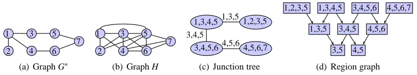
Figure 1: Our framework for estimating the graph in (a) using (b) computes the junction tree in (c) and uses a region graph representation in (d) of the junction tree to decompose the UGMS problem into multiple subproblems.
then (j, i) ∈ E(G∗). The undirected graphical model selection (UGMS) problem is to estimate G∗ given n observations Xn = X(1), . . . , X(n) drawn from P
X. This problem is
of interest in many areas including biological data analysis, financial analysis, and social network analysis; see Koller and Friedman (2009) for some more examples.
This paper studies the following problem: Given the observations Xn
drawn from PX and a graph H that contains all the true edges E(G∗), and
possibly some extra edges, estimate the graph G∗.
A natural question to ask is how can the graph H be selected in the first place? One way of doing so is to use screening algorithms, such as in Fan and Lv (2008) or in Vats (to appear), to eliminate edges that are clearly non-existent in G∗. Another method can be to use partial prior information about X to remove unnecessary edges. For example, this could be based on (i) prior knowledge about statistical properties of genes when analyzing gene expressions, (ii) prior knowledge about companies when analyzing stock returns, or (iii) demographic information when modeling social networks. Yet another method can be to use clever model selection algorithms that estimate more edges than desired. Assuming an initial graphH has been computed, our main contribution in this paper is to show how a junction tree representation ofH can be used as a wrapper around UGMS algorithms for more accurate graph estimation.
1.1 Overview of the Junction Tree Framework
A junction tree is a tree-structured representation of an arbitrary graph (Robertson and Seymour, 1986). The vertices in a junction tree are clusters of vertices from the original graph. An edge in a junction tree connects two clusters. Junction trees are used in many applications to reduce the computational complexity of solving graph related problems (Arnborg and Proskurowski, 1989). Figure 1(c) shows an example of a junction tree for the graph in Figure 1(b). Notice that each edge in the junction tree is labeled by the set of vertices common to both clusters connected by the edge. These set of vertices are referred to as a separator.
Let H be a graph that contains all the edges in G∗. We show that the UGMS problem can be decomposed into multiple subproblems over clusters and subsets of the separators in a junction tree representation ofH. In particular, using the junction tree, we construct
A Junction Tree Framework for Undirected Graphical Model Selection
Journal of Machine Learning Research () Submitted 4/13; Revised 9/13; Published
-T V1
V2
c
Divyanshu Vats and Robert D. Nowak.
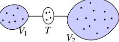
Figure 2: Structure of the graph used to analyze the junction tree framework for UGMS.
a region graph, which is a directed graph over clusters of vertices. An example of a region graph for the junction tree in Figure 1(c) is shown in Figure 1(d). The first two rows in the region graph are the clusters and separators of the junction tree, respectively. The rest of the rows contain subsets of the separators.1 The multiple subproblems we identify correspond
to estimating a subset of edges over each cluster in the region graph. For example, the subproblem over the cluster{1,2,3,5} in Figure 1(d) estimates the edges (2,3) and (2,5).
We solve the subproblems over the region graph in an iterative manner. First, all subproblems in the first row of the region graph are solved in parallel. Second, the region graph is updated taking into account the edges removed in the first step. We keep solving subproblems over rows in the region graph and update the region graph until all the edges in the graph H have been estimated.
As illustrated above, our framework depends on a junction tree representation of the graphHthat contains a superset of the true edges. Given any graph, there may exist several junction tree representations. An optimal junction tree is a junction tree representation such that the maximum size of the cluster is as small as possible. Since we apply UGMS algorithms to the clusters of the junction tree, and the complexity of UGMS depends on the number of vertices in the graph, it is useful to apply our framework using optimal junction trees. Unfortunately, it is computationally intractable to find optimal junction trees (Arnborg et al., 1987). However, there exists several computationally efficient greedy heuristics that compute close to optimal junction trees (Kjaerulff, 1990; Berry et al., 2003). We use such heuristics to find junction trees when implementing our algorithms in practice.
1.2 Advantages of Using Junction Trees
We highlight three main advantages of the junction tree framework for UGMS.
Choosing Regularization Parameters and UGMS Algorithms: UGMS algorithms typically depend on a regularization parameter that controls the number of estimated edges. This regularization parameter is usually chosen using model selection algorithms such as cross-validation or stability selection. Since each subproblem we identify in the region graph is solved independently, different regularization parameters can be used to learn different parts of the graph. This has advantages when the true graph G∗ has different charac-teristics in different parts of the graph. Further, since the subproblems are independent, different UGMS algorithms can be used to learn different parts of the graph. Our numerical simulations clearly show the advantages of this property.
Reduced Sample Complexity: One of the key results of our work is to show that in many cases, the junction tree framework is capable of consistently estimating a graph under weaker conditions than required by previously proposed methods. For example, we show that if
Vats and Nowak
G∗ consists of two main components that are separated by a relatively small number of vertices (see Figure 2 for a general example), then, under certain conditions, the number of observations needed for consistent estimation scales like log(pmin), wherepminis the number
of vertices in the smaller of the two components. In contrast, existing methods are known to be consistent if the observations scale like logp, wherepis the total number of vertices. If the smaller component were, for example, exponentially smaller than the larger component, then the junction tree framework is consistent with about log logpobservations. For generic problems, without structure that can be exploited by the junction tree framework, we recover the standard conditions for consistency.
Learning Weak Edges: A direct consequence of choosing different regularization parameters and the reduced sample complexity is that certain weak edges, not estimated using standard algorithms, may be estimated when using the junction tree framework. We show this theoretically and using numerical simulations on both synthetic and real world data.
1.3 Related Work
Several algorithms have been proposed in the literature for learning undirected
graph-ical models. Some examples include References Spirtes and Glymour (1991), Kalisch
and B¨uhlmann (2007), Banerjee et al. (2008), Friedman et al. (2008), Meinshausen and B¨uhlmann (2006), Anandkumar et al. (2012a) and Cai et al. (2011) for learning Gaussian graphical models, references Liu et al. (2009), Xue and Zou (2012), Liu et al. (2012a), Laf-ferty et al. (2012) and Liu et al. (2012b) for learning non-Gaussian graphical models, and references Bresler et al. (2008), Bromberg et al. (2009), Ravikumar et al. (2010), Netrapalli et al. (2010), Anandkumar et al. (2012b), Jalali et al. (2011), Johnson et al. (2012) and Yang et al. (2012) for learning discrete graphical models. Although all of the above algorithms can be modified to take into account prior knowledge about a graphH that contains all the true edges (see Appendix B for some examples), our junction tree framework is fundamen-tally different than the standard modification of these algorithms. The main difference is that the junction tree framework allows for using theglobal Markov property of undirected graphical models (see Definition 1) when learning graphs. This allows for improved graph estimation, as illustrated by both our theoretical and numerical results. We note that all of the above algorithms can be used in conjunction with the junction tree framework.
Junction trees have been used for performing exact probabilistic inference in graphical models (Lauritzen and Spiegelhalter, 1988). In particular, given a graphical model, and its junction tree representation, the computational complexity of exact inference is expo-nential in the size of the cluster in the junction tree with the most of number of vertices. This has motivated a line of research for learning thin junction trees so that the maximum size of the cluster in the estimated junction tree is small so that inference is computa-tionally tractable (Chow and Liu, 1968; Bach and Jordan, 2001; Karger and Srebro, 2001; Chechetka and Guestrin, 2007; Kumar and Bach, 2013). We also make note of algorithms for learning decomposable graphical models where the graph structure is assumed to tri-angulated (Malvestuto, 1991; Giudici and Green, 1999). In general, the goal in the above algorithms is to learn a joint probability distribution that approximates a more complex probability distribution so that computations, such as inference, can be done in a tractable manner. On the other hand, this paper considers the problem of learning the structure of
A Junction Tree Framework for Undirected Graphical Model Selection
the graph that best represents the conditional dependencies among the random variables under consideration.
There are two notable algorithms in the literature that use junction trees for learning graphical models. The first is an algorithm presented in Xie and Geng (2008) that uses junction trees to find the direction of edges for learning directed graphical models. Unfor-tunately, this algorithm cannot be used for UGMS. The second is an algorithm presented in Ma et al. (2008) for learning chain graphs, that are graphs with both directed and undi-rected edges. The algorithm in Ma et al. (2008) uses a junction tree representation to learn an undirected graph before orienting some of the edges to learn a chain graph. Our pro-posed algorithm, and subsequent analysis, differs from the work in Ma et al. (2008) in the following ways:
(i) Our algorithm identifies an ordering on the edges, which subsequently results in a lower sample complexity and the possibility of learning weak edges in a graph. The ordering on the edges is possible because of our novel region graph interpretation for learning graphical models. For example, when learning the graph in Figure 1(a) using Figure 1(b), the algorithm in Ma et al. (2008) learns the edge (3,5) by applying a UGMS algorithm to the vertices{1,2,3,4,5,6}. In contrast, our proposed algorithm first estimates all edges in the second layer of the region graph in Figure 1(d), re-estimates the region graph, and then only applies a UGMS algorithm to {3,4,5} to determine if the edge (3,4) belongs to the graph. In this way, our algorithm, in general, requires applying a UGMS algorithm to a smaller number of vertices when learning edges over separators in a junction tree representation.
(ii) Our algorithm for using junction trees for UGMS is independent of the choice of the UGMS algorithm, while the algorithm presented in Ma et al. (2008) uses conditional independence tests for UGMS.
(iii) Our algorithm, as discussed in (i), has the additional advantage of learning certain weak edges that may not be estimated when using standard UGMS algorithms. We theoretically quantify this property of our algorithm, while no such theory was pre-sented in Ma et al. (2008).
Vats and Nowak
1.4 Paper Organization
The rest of the paper is organized as follows:
• Section 2 reviews graphical models and formulates the undirected graphical model selection (UGMS) problem.
• Section 3 shows how junction trees can be represented as region graphs and outlines an algorithm for constructing a region graph from a junction tree.
• Section 4 shows how the region graphs can be used to apply a UGMS algorithm to the clusters and separators of a junction tree.
• Section 5 presents our main framework for using junction trees for UGMS. In partic-ular, we show how the methods in Sections 3-4 can be used iteratively to estimate a graph.
• Section 6 reviews the PC-Algorithm, which we use to study the theoretical properties of the junction tree framework.
• Section 7 presents theoretical results on the sample complexity of learning graphical models using the junction tree framework. We also highlight advantages of using the junction tree framework as summarized in Section 1.2.
• Section 8 presents numerical simulations to highlight the advantages of using junction trees for UGMS in practice.
• Section 9 summarizes the paper and outlines some future work.
2. Preliminaries
In this section, we review some necessary background on graphs and graphical models that we use in this paper. Section 2.1 reviews some graph theoretic concepts. Section 2.2 reviews undirected graphical models. Section 2.3 formally defines the undirected graphical model selection (UGMS) problem. Section 2.4 reviews junction trees, which we use use as a tool for decomposing UGMS into multiple subproblems.
2.1 Graph Theoretic Concepts
A graph is a tuple G = (V, E(G)), where V is a set of vertices and E(G) ⊆ V ×V are edges connecting vertices in V. For any graph H, we use the notation E(H) to denote its edges. We only consider undirected graphs where if (v1, v2)∈ E(G), then (v2, v1) ∈E(G)
for v1, v2 ∈V. Some graph theoretic notations that we use in this paper are summarized
as follows:
• NeighborneG(i): Set of nodes connected to i.
• Path {i, s1, . . . , sd, j}: A sequence of nodes such that (i, s1),(sd, j),(sk, sk+1)∈E for
k= 1, . . . , d−1.
A Junction Tree Framework for Undirected Graphical Model Selection
• SeparatorS: A set of nodes such that all paths from itoj contain at least one node inS. The separatorS isminimal if no proper subset of S separatesi andj.
• Induced SubgraphG[A] = (A, E(G[A])): A graph over the nodesAsuch thatE(G[A]) contains the edges only involving the nodes inA.
• Complete graphKA: A graph that contains all possible edges over the nodes A.
For two graphsG1 = (V1, E(G1)) andG2= (V2, E(G2)), we define the following standard
operations:
• Graph Union: G1∪G2 = (V1∪V2, E1∪E2).
• Graph Difference: G1\G2 = (V1, E1\E2).
2.2 Undirected Graphical Models
Definition 1 (Undirected Graphical Model, Lauritzen, 1996) An undirected graph-ical model is a probability distribution PX defined on a graph G∗ = (V, E(G∗)), where
V = {1, . . . , p} indexes the random vector X = (X1, . . . , Xp) and the edges E(G∗) encode
the following Markov property: for a set of nodes A, B, and S, if S separates A and B, thenXA⊥⊥XB|XS.
The Markov property outlined above is referred to as theglobal Markov property. Undirected graphical models are also referred to as Markov random fields or Markov networks in the literature. When the joint probability distribution PX is non-degenerate, that is, PX >
0, the Markov property in Definition 1 are equivalent to the pairwise and local Markov properties:
• Pairwise Markov property: For all (i, j)∈/ E,Xi ⊥⊥Xj|XV\{i,j}.
• Local Markov property: For alli∈V,Xi⊥⊥XV\{neG(i)∪{i}}|XneG(i).
In this paper, we always assume PX > 0 and say PX is Markov on G to reflect the
Markov properties. Examples of conditional independence relations conveyed by a proba-bility distribution defined on the graph in Figure 3(d) are X1 ⊥⊥ X6|{X2, X4} and X4 ⊥⊥
X6|{X2, X5, X8}.
2.3 Undirected Graphical Model Section (UGMS)
Definition 2 (UGMS) The undirected graphical model selection (UGMS) problem is to estimate a graph G∗ such that the joint probability distribution PX is Markov on G∗, but
not Markov on any subgraph of G∗.
The last statement in Definition 2 is important, since, if PX is Markov on G∗, then it is
Vats and Nowak
Let Ψ be an abstract UGMS algorithm that takes as inputs a set of ni.i.d. observations
Xn={X(1), . . . , X(n)}drawn fromP
X and a regularization parameterλn. The output of Ψ
is a graphGbn, whereλncontrols the number of edges estimated inGbn. Note the dependence
of the regularization parameter onn. We assume Ψ is consistent, which is formalized in the following assumption.
Assumption 1 There exists a λn for which P(Gbn = G∗) → 1 as n → ∞, where Gbn =
Ψ(Xn, λ n).
We give examples of Ψ in Appendix B. Assumption 1 also takes into account the high-dimensional case wherep depends onnin such a way thatp, n→ ∞.
2.4 Junction Trees
Junction trees (Robertson and Seymour, 1986) are used extensively for efficiently solving various graph related problems, see Arnborg and Proskurowski (1989) for some examples. Reference Lauritzen and Spiegelhalter (1988) shows how junction trees can be used for exact inference (computing marginal distribution given a joint distribution) over graphical models. We use junction trees as a tool for decomposing the UGMS problem into multiple subproblems.
Definition 3 (Junction tree) For an undirected graph G = (V, E(G)), a junction tree J = (C, E(J))is a tree-structured graph over clusters of nodes in V such that
(i) Each node in V is associated with at least one cluster inC.
(ii) For every edge(i, j)∈E(G), there exists a clusterCk∈ C such that i, j∈Ck.
(iii) J satisfies the running intersection property: For all clusters Cu, Cv, and Cw such
that Cw separates Cu and Cv in the tree defined byE(J), Cu∩Cv ⊂Cw.
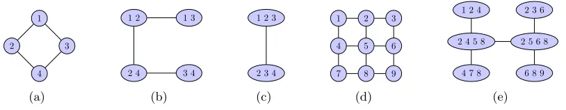
The first property in Definition 3 says that all nodes must be mapped to at least one cluster of the junction tree. The second property states that each edge of the original graph must be contained within a cluster. The third property, known as the running intersection property, is the most important since it restricts the clusters and the trees that can be be formed. For example, consider the graph in Figure 3(a). By simply clustering the nodes over edges, as done in Figure 3(b), we cannot get a valid junction tree (Wainwright, 2002). By making appropriate clusters of size three, we get a valid junction tree in Fig. 3(c). In other words, the running intersection property says that for two clusters with a common node, all the clusters on the path between the two clusters must contain that common node.
Proposition 4 (Robertson and Seymour, 1986) LetJ = (C, E(J))be a junction tree of the graph G. LetSuv=Cu∩Cv. For each(Cu, Cv)∈ E, we have the following properties:
1. Suv6=∅.
2. Suv separates Cu\Suv and Cv\Suv.
A Junction Tree Framework for Undirected Graphical Model Selection
1
2 3
4
(a)
1 3 1 2
2 4 3 4
(b)
1 2 3
2 3 4
(c)
1 2 3
4 5 6
7 8 9
(d)
1 2 4
2 4 5 8
4 7 8
2 5 6 8 2 3 6
6 8 9
(e)
Figure 3: (a) An undirected graph, (b) Invalid junction tree since {1,2} separates {1,3} and{3,4},but 3∈ {/ 1,2}. (c) Valid junction tree for the graph in (a). (d) A grid graph. (e) Junction tree representation of (d).
The set of nodes Suv on the edges are called theseparators of the junction tree.
Propo-sition 4 says that all clusters connected by an edge in the junction tree have at least one common node and the common nodes separate nodes in each cluster. For example, consider the junction tree in Figure 3(e) of the graph in Figure 3(d). We can infer that 1 and 5 are separated by 2 and 4. Similarly, we can also infer that 4 and 6 are separated by 2, 5, and 8. It is clear that if a graphical model is defined on the graph, then the separators can be used to easily define conditional independence relationships. For example, using Figure 3(e), we can conclude thatX1 ⊥⊥X5 givenX2 andX4. As we will see in later Sections, Proposition 4
allow the decomposition of UGMS into multiple subproblems over clusters and subsets of the separators in a junction tree.
3. Overview of Region Graphs
In this section, we show how junction trees can be represented as region graphs. As we will see in Section 5, region graphs allow us to easily decompose the UGMS problem into multiple subproblems. There are many different types of region graphs and we refer the readers to Yedidia et al. (2005) for a comprehensive discussion about region graphs and how they are useful for characterizing graphical models. The region graph we present in this section differs slightly from the standard definition of region graphs. This is mainly because our goal is to estimate edges, while the standard region graphs defined in the literature are used for computations over graphical models.
A region is a collection of nodes, which in this paper can be the clusters of the junction tree, separators of the junction tree, or subsets of the separators. A region graph G = (R, ~E(G)) is a directed graph where the vertices are regions and the edges represent directed edges from one region to another. We use the notationE~(·) to emphasize that region graphs contain directed edges. A description of region graphs is given as follows:
• The set E~(G) contains directed edges so that if (R, S) ∈ E~(G), then there exists a directed edge from region R to regionS.
• Whenever R−→S, thenS ⊆R.
Vats and Nowak
Journal of Machine Learning Research () Submitted 4/13; Revised 9/13; Published
-1
2
3 5
6
7 4
8
9
(a)
5,6,8,9
3,4,6,7 2,3,4,6
1,3,5
2,3,5,6
3,5,6,8 3,5
5,6,8 3,5,6
2,3,6
3,4,6
C1
C2
C3
C4
C5 C6
(b) Junction tree
1,3,5 3,5,6,8 5,6,8,9 2,3,5,6 2,3,4,6 3,4,6,7
3,5,6 5,6,8 2,3,6 3,4,6
3,5 5,6 3,6 3,5
(c) Region graph
c
Divyanshu Vats and Robert D. Nowak.
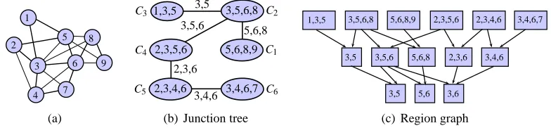
Figure 4: (a) An example ofH. (b) A junction tree representation ofH. (c) A region graph representation of (b) computed using Algorithm 1.
Algorithm 1:Constructing region graphs
Input: A junction treeJ = (C, E(J)) of a graph H. Output: A region graphG = (R, ~E(G)).
1 R1 =C, whereC are the clusters of the junction tree J.
2 LetR2 be all the separators ofJ, that is,R2 ={Suv =Cu∩Cv : (Cu, Cv)∈E(J)}.
3 To constructR3, find all possible pairwise intersections of regions in R2. Add all
intersecting regions with cardinality greater than one to R3.
4 Repeat previous step to construct R4, . . . ,RL until there are no more intersecting
regions of cardinality greater than one.
5 For R∈ R` andS ∈ R`+1, add the edge (R, S) to E~(G) if S⊆R. 6 Let R={R1, . . . ,RL}.
regions with the same label to partition R intoL groups R1, . . . ,RL. In Algorithm 1, we
initialize R1 and R2 to be the clusters and separators of a junction tree J, respectively,
and then iteratively findR3, . . . ,RLby computing all possible intersections of regions with
the same label. The edges in E~(G) are only drawn from a region in Rl to a region in
Rl+1. Figure 4(c) shows an example of a region graph computed using the junction tree in
Figure 4(b).
Remark 5 Note that the construction of the region graph depends on the junction tree. Using methods in Vats and Moura (2012), we can always construct junction trees such that the region graph only has two sets of regions, namely the clusters of the junction tree and the separators of the junction tree. However, in this case, the size of the regions or clusters may be too large. This may not be desirable since the computational complexity of applying UGMS algorithms to region graphs, as shown in Section 5, depends on the size of the regions.
Remark 6 (Region graph vs. Junction tree) For every junction tree, Algorithm 1 outputs a unique region graph. The junction tree only characterizes the relationship between the clusters in a junction tree. A region graph extends the junction tree representation to characterize the relationships between the clusters as well as the separators. For example, in Figure 4(c), the region{5,6}is in the third row and is a subset of two separators of the
A Junction Tree Framework for Undirected Graphical Model Selection
junction tree. Thus, the only difference between the region graph and the junction tree is the additional set of regions introduced inR3, . . . ,RL.
Remark 7 From the construction in Algorithm 1, R may have two or more regions that are the same but have different labels. For example, in Figure 4(c), the region {3,5} is in both R2 and R3. We can avoid this situation by removing {3,5} from R2 and adding an
edge from the region {1,3,5} in R1 to the region {3,5} in R3. For notational simplicity
and for the purpose of illustration, we allow for duplicate regions. This does not change the theory or the algorithms that we develop.
4. Applying UGMS to Region Graphs
Before presenting our framework for decomposing UGMS into multiple subproblems, we first show how UGMS algorithms can be applied to estimate a subset of edges in a region of a region graph. In particular, for a region graph G = (R, ~E(G)), we want to identify a set of edges in the induced subgraph H[R]that can be estimated by applying a UGMS algorithm to either R or a set of vertices that containsR. With this goal in mind, define the children ch(R) of a region R as follows:
Children: ch(R) =nS: (R, S)∈E~o. (1)
We say R connects to S if (R, S) ∈ E~(G). Thus, the children in (1) consist of all regions thatR connects to. For example, in Figure 4(c),
ch({2,3,4,6}) ={{2,3,6},{3,4,6}}.
If there exists a direct path from S to R, we say S is an ancestor of R. The set of all ancestors of R is denoted byan(R). For example, in Figure 4(c),
an({5,6,8,9}) =∅,
an({3,5,6}) ={{3,5,6,8},{2,3,5,6}},and
an({3,6}) ={{3,5,6},{2,3,6},{3,4,6},{2,3,5,6},{2,3,4,6},{3,4,6,7},{3,5,6,8}}}.
The notationR takes the union of all regions in an(R) and R so that
R= [
S∈{an(R),R}
S . (2)
Thus,Rcontains the union of all clusters in the junction tree that containR. An illustration of some of the notations defined on region graphs is shown in Figure 5. Usingch(R), define the subgraphHR0 as2
HR0 =H[R]\∪S∈ch(R)KS , (3)
whereH[R] is the induced subgraph that contains all edges inH over the regionR andKS
is the complete graph over S. In words,H0
R is computed by removing all edges from H[R]
that are contained in another separator. For example, in Figure 4(c), when R ={5,6,8}, E(H0
R) = {(5,8),(6,8)}. The subgraph HR0 is important since it identifies the edges that
can be estimated when applying a UGMS algorithm to the set of vertices R.
Vats and Nowak
Algorithm 2:UGMS over regions in a region graph
1: Input: Region graphG= (R, ~E(G)), a regionR, observationsXn, and a UGMS
algorithm Ψ.
2: Compute HR0 using (3) andR using (2). 3: Apply Ψ toXn
R to estimate edges inH
0
R. See Appendix B for examples.
4: Returnthe estimated edges EbR.
Journal of Machine Learning Research () Submitted 4/13; Revised 9/13; Published
-R
ch(R)
an(R)
c
Divyanshu Vats and Robert D. Nowak.
Figure 5: Notations defined on region graphs. The children ch(R) are the set of regions thatR connects to. The ancestorsan(R) are all the regions that have a directed path to the regionR. The setR takes the union of all regions inan(R) andR.
Proposition 8 Suppose E(G∗) ⊆ E(H). All edges in HR0 can be estimated by solving a UGMS problem over the vertices R.
Proof See Appendix C.
Proposition 8 says that all edges inHR0 can be estimated by applying a UGMS algorithm to the set of vertices R. The intuition behind the result is that only those edges in the region R can be estimated whose Markov properties can be deduced using the vertices in R. Moreover, the edgesnot estimated inH[R] share an edge with another region that does not contain all the vertices inR. Algorithm 2 summarizes the steps involved in estimating the edges in HR0 using the UGMS algorithm Ψ defined in Section 2.3. Some examples on how to use Algorithm 2 to estimate some edges of the graph in Figure 4(a) using the region graph in Figure 4(c) are described as follows.
1. Let R = {1,3,5}. This region only connects to {3,5}. This means that all edges, except the edge (3,5) inH[R], can be estimated by applying Ψ toR.
2. LetR={3,5,6}. The children of this region are{3,5},{5,6}, and{3,6}. This means thatHR0 =∅, that is, no edge over H[R] can be estimated by applying Ψ to{3,5,6}.
A Junction Tree Framework for Undirected Graphical Model Selection
Notation Description
G∗= (V, E(G∗)) Unknown graph that we want to estimate.
H Known graph such that E(G∗)⊆E(H).
G= (R, ~E(G)) Region graph of H constructed using Algorithm 1. R= (R1, . . . ,RL) Partitioning of the regions inRinto Llabels.
R The set of vertices used when applying Ψ to estimate edges overR.
See (2) for definition.
HR0 Edges in H[R] that can be estimated using Algorithm 2.
See (3) for definition.
Table 1: A summary of some notations.
3. Let R = {3,4,6}. This region only connects to {3,6}. Thus, all edges except (3,6) can be estimated. The regions{2,3,4,6} and {3,4,6,7} connect toR, so Ψ needs to be applied toR ={2,3,4,6,7}.
5. UGMS Using Junction Trees: A General Framework
In this section, we present the junction tree framework for UGMS using the results from Sections 3-4. Section 5.1 presents the junction tree framework. Section 5.2 discusses the computational complexity of the framework. Section 5.3 highlights the advantages of using junction trees for UGMS using some examples. We refer to Table 1 for a summary of all the notations that we use in this section.
5.1 Description of Framework
Recall that Algorithm 2 shows that to estimate a subset of edges in H[R], where R is a region in the region graphG, the UGMS algorithm Ψ in Assumption 1 needs to be applied to the set R defined in (2). Given this result, a straightforward approach to decomposing the UGMS problem is to apply Algorithm 2 to each regionRand combine all the estimated edges. This will work since for any R, S ∈ R such that R 6= S, E(HR0 )∩E(HS0) = ∅. This means that each application of Algorithm 2 estimates a different set of edges in the graph. However, for some edges, this may require applying a UGMS algorithm to a large set of nodes. For example, in Figure 4(c), when applying Algorithm 2 to R ={3,6}, the UGMS algorithm needs to be applied toR={2,3,4,5,6,7,8}, which is almost the full set of vertices. To reduce the problem size of the subproblems, we apply Algorithms 1 and 2 in an iterative manner as outlined in Algorithm 3.
Vats and Nowak
Journal of Machine Learning Research () Submitted 4/13; Revised 9/13; Published
-Apply UGMS to a row of region graph
(Algorithm 2) Find Junction Tree
and Region Graph (Algorithm 1)
Have all edges
been estimated? Xn,H
Output graph No
Yes
c
Divyanshu Vats and Robert D. Nowak.
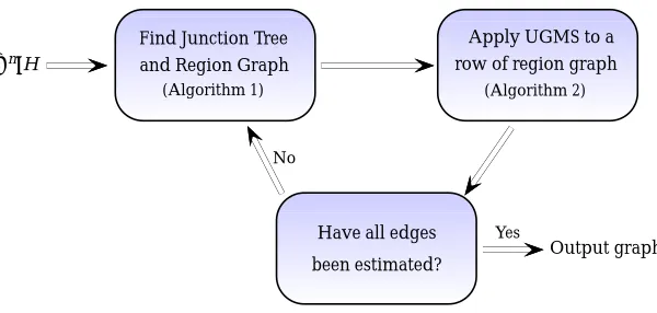
Figure 6: A high level overview of the junction tree framework for UGMS in Algorithm 3.
Algorithm 3:Junction Tree Framework for UGMS See Table 1 for notations.
Step 1. Initialize Gb so thatE(Gb) =∅and find the region graph G ofH.
Step 2. Find the smallest `such that there exists a regionR∈ R` such thatE(H0
R)6=∅.
Step 3. Apply Algorithm 2 to each region in R`.
Step 4. Add all estimated edges to Gb and remove edges from H that have been estimated. NowH∪Gb contains all the edges in G∗.
Step 5. Compute a new junction tree and region graph G using the graph Gb∪H. Step 6. If E(H) =∅, stop the algorithm, else go to Step 2.
all the edges inG∗. We repeat the above steps on a new region graph computed usingGb∪H and stop the algorithm when H is an empty graph.
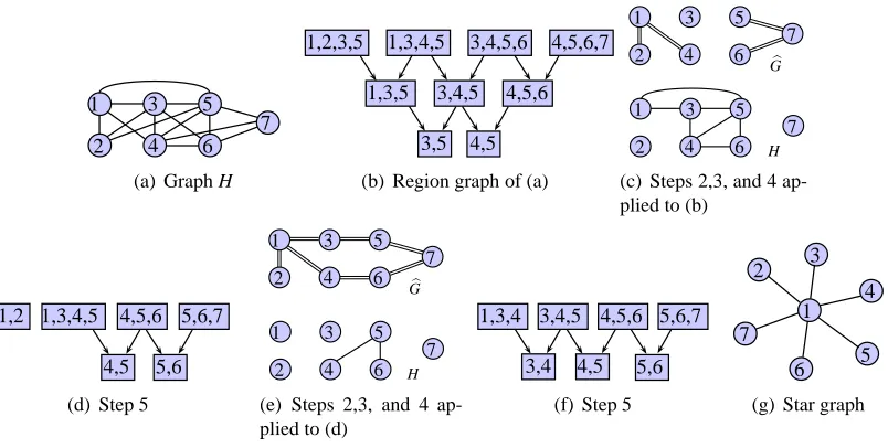
An example illustrating the junction tree framework is shown in Figure 7. The region graph in Figure 7(b) is constructed using the graph H in Figure 7(a). The true graph G∗ we want to estimate is shown in Figure 1(a). The top and bottom in Figure 7(c) show the graphsGbandH, respectively, after estimating all the edges inR1of Figure 7(b). The edges
inGb are represented by double lines to distinguish them from the edges in H. Figure 7(d) shows the region graph ofGb∪H. Figure 7(e) shows the updated Gb and H where only the edges (4,5) and (5,6) are left to be estimated. This is done by applying Algorithm 2 to the regions in R2 of Figure 7(f). Notice that we did not include the region {1,2} in the
last region graph since we know all edges in this region have already been estimated. In general, ifE(H[R]) =∅for any regionR, we can remove this region and thereby reduce the computational complexity of constructing region graphs.
A Junction Tree Framework for Undirected Graphical Model Selection
Journal of Machine Learning Research () Submitted 4/13; Revised 9/13; Published
-1 2 4 3 6 5 7
(a) Graph H
1,2,3,5 1,3,4,5 3,4,5,6 4,5,6,7
1,3,5 3,4,5 4,5,6
3,5 4,5
(b) Region graph of (a)
1 2 4 3 6 5 7 1 2 4 3 6 5 7 G H
(c) Steps 2,3, and 4 ap-plied to (b)
1,3,4,5 4,5,6 1,2
4,5
5,6,7
5,6
(d) Step 5
1 2 4 3 6 5 7 1 2 4 3 6 5 7 G H
(e) Steps 2,3, and 4 ap-plied to (d)
4,5,6 3,4 5,6,7 4,5 1,3,4 3,4,5 5,6
(f) Step 5
1 2 4 3 6 5 7
(g) Star graph
c
Divyanshu Vats and Robert D. Nowak.
Figure 7: Example to illustrate the junction tree framework in Algorithm 3.
5.2 Computational Complexity
In this section, we discuss the computational complexity of the junction tree framework. It is difficult to write down a closed form expression since the computational complexity depends on the structure of the junction tree. Moreover, merging clusters in the junction tree can easily control the computations. With this in mind, the main aim in this section is to show that the complexity of the framework is roughly the same as that of applying a standard UGMS algorithm. Consider the following observations.
1. Computing H: Assuming no prior knowledge about H is given, this graph needs to be computed from the observations. This can be done using standard screening algorithms, such as those in Fan and Lv (2008) and Vats (to appear), or by applying a UGMS algorithm with a regularization parameter that selects a larger number of edges (than that computed by using a standard UGMS algorithm). Thus, the complexity of computingHis roughly the same as that of applying a UGMS algorithm to all the vertices in the graph.
2. Applying UGMS to regions: Recall from Algorithm 2 that we apply a UGMS algorithm to observations over R to estimate edges over the vertices R, where R is a region in a region graph representation of H. Since |R| ≤p, it is clear that the complexity of Algorithm 2 is less than that of applying a UGMS algorithm to estimate all edges in the graph.
Vats and Nowak
since there can be an exponential number of possible junction tree representations. Alternatively, we can select a junction tree so that the maximum size of the clusters is as small as possible. Such junction trees are often referred to as optimal junction trees in the literature. Although finding optimal junction trees is also hard (Arnborg et al., 1987), there exists several computationally tractable heuristics for finding close to optimal junction trees (Kjaerulff, 1990; Berry et al., 2003). The complexity of such algorithms range from O(p2) to O(p3), depending on the degree of approximation.
We note that this time complexity is less than that of standard UGMS algorithms.
It is clear that the complexity of all the intermediate steps in the framework is less than that of applying a standard UGMS algorithm. The overall complexity of the framework depends on the number of clusters in the junction tree and the size of the separators in the junction tree. The size of the separators in a junction tree can be controlled by merging clusters that share a large separator. This step can be done in linear time. Removing large separators also reduces the total number of clusters in a junction tree. In the worst case, if all the separators in H are too large, the junction tree will only have one cluster that contains all the vertices. In this case, using the junction tree framework will be no different than using a standard UGMS algorithm.
5.3 Advantages of using Junction Trees and Region Graphs
An alternative approach to estimating G∗ using H is to modify some current UGMS algo-rithms (see Appendix B for some concrete examples). For example, neighborhood selection based algorithms first estimate the neighborhood of each vertex and then combine all the estimated neighborhoods to construct an estimate Gb of G∗ (Meinshausen and B¨uhlmann, 2006; Bresler et al., 2008; Netrapalli et al., 2010; Ravikumar et al., 2010). Two ways in which these algorithms can be modified when givenH are described as follows:
1. A straightforward approach is to decompose the UGMS problem intop different sub-problems of estimating the neighborhood of each vertex. The graph H can be used to restrict the estimated neighbors of each vertex to be subsets of the neighbors inH. For example, in Figure 7(a), the neighborhood of 1 is estimated from the set{2,3,4,5} and the neighborhood of 3 is estimated from the set{1,4,5,6}. This approach can be compared to independently applying Algorithm 2 to each region in the region graph. For example, when using the region graph, the edge (1,4) can be estimated by apply-ing a UGMS algorithm to {1,3,4,5}. In comparison, when not using region graphs, the edge (1,4) is estimated by applying a UGMS algorithm to{1,2,3,4,5}. In general, using region graphs results in smaller subproblems. A good example to illustrate this is the star graph in Figure 7(g). A junction tree representation of the star graph can be computed so that all clusters will have size two. Subsequently, the junction tree framework will only require applying a UGMS algorithm to a pair of nodes. On the other hand, neighborhood selection needs to be applied to all the nodes to estimate the neighbors of the central node 1 which is connected to all other nodes.
2. An alternative approach is to estimate the neighbors of each vertex in an iterative manner. However, it is not clear what ordering should be chosen for the vertices. The
A Junction Tree Framework for Undirected Graphical Model Selection
region graph approach outlined in Section 5.1 leads to a natural choice for choosing which edges to estimate in the graph so as to reduce the problem size of subsequent subproblems. Moreover, iteratively applying neighborhood selection may still lead to large subproblems. For example, suppose the star graph in Figure 7(g) is in fact the true graph. In this case, using neighborhood selection always leads to applying UGMS to all the nodes in the graph.
From the above discussion, it is clear that using junction trees for UGMS leads to smaller subproblems and a natural choice of an ordering for estimating edges in the graph. We will see in Section 7 that the smaller subproblems lead to weaker conditions on the number of observations required for consistent graph estimation. Moreover, our numerical simulations in Section 8 empirically show the advantages of using junction tree over neighborhood selection based algorithms.
6. PC-Algorithm for UGMS
So far, we have presented the junction tree framework using an abstract undirected graph-ical model selection (UMGS) algorithm. This shows that our framework can be used in conjunction with any UGMS algorithm. In this section, we review the PC-Algorithm, since we use it to analyze the junction tree framework in Section 7. The PC-Algorithm was originally proposed in the literature for learning directed graphical models (Spirtes and Glymour, 1991). The first stage of the PC-Algorithm, which we refer to asPC, estimates an undirected graph using conditional independence tests. The second stage orients the edges in the undirected graph to estimate a directed graph. We use the first stage of the PC-Algorithm for UGMS. PC-Algorithm 4 outlinesPC. Variants of the PC-Algorithm for learning undirected graphical models have recently been analyzed in Anandkumar et al. (2012b,a). The main property used inPCis the global Markov property of undirected graphical models which states that if a set of vertices S separates i and j, then Xi ⊥⊥ Xj|XS. As seen in
Line 5 of Algorithm 4, PC deletes an edge (i, j) if it identifies a conditional independence relationship. Some properties of PCare summarized as follows:
1. Parameterκ: PCiteratively searches for separators for an edge (i, j) by searching for separators of size 0,1, . . . , κ. This is reflected in Line 2 of Algorithm 4. Theoretically, the algorithm can automatically stop after searching for all possible separators for each edge in the graph. However, this may not be computationally tractable, which is whyκ needs to be specified.
2. Conditional Independence Test: Line 5 of Algorithm 4 uses a conditional indepen-dence test to determine if an edge (i, j) is in the true graph. This makesPCextremely flexible since nonparametric independence tests may be used, see Hoeffding (1948), Rasch et al. (2012) and Zhang et al. (2012) for some examples. In this paper, for simplicity, we only consider Gaussian graphical models. In this case, conditional in-dependence can be tested using the conditional correlation coefficient defined as
Conditional correlation coefficient: ρij|S =
Σij −Σi,SΣ−S,S1ΣS,j
p
Σi,i|SΣj,j|S
Vats and Nowak
Algorithm 4:PC-Algorithm for UGMS:PC(κ,Xn, H, L)
Inputs:
κ: An integer that controls the computational complexity of PC.
Xn: ni.i.d. observations.
H: A graph that contains all the true edges G∗.
L: A graph that contains the edges that need to be estimated.
Output: A graphGb that contains edges in L that are estimated to be inG∗.
1 Gb←L
2 for each k∈ {0,1, . . . , κ} do 3 foreach (i, j)∈E(Gb) do
4 Sij ← Neighbors ofiorj inH depending on which one has lower cardinality. 5 if ∃ S⊂ Sij, |S|=k, s.t. Xi ⊥⊥Xj|XS (computed using Xn) then
6 Delete edge (i, j) fromGb andH.
7 Return Gb.
wherePX ∼ N(0,Σ), ΣA,B is the covariance matrix ofXAandXB, and ΣA,B|S is the
conditional covariance defined by
ΣA,B|S = ΣA,B−ΣA,SΣ−S,S1ΣB,S.
Whenever Xi ⊥⊥ Xj|XS, then ρij|S = 0. This motivates the following test for
inde-pendence:
Conditional Independence Test: |ρbij|S|< λn=⇒Xi ⊥⊥Xj|XS, (4)
whereρbij|S is computed using the empirical covariance matrix from the observations Xn. The regularization parameter λ
n controls the number of edges estimated inGb.
3. The graphsHandL: Recall thatHcontains all the edges inG∗. The graphLcontains edges that need to be estimated since, as seen in Algorithm 2, we apply UGMS to only certain parts of the graph instead of the whole graph. As an example, to estimate edges in a region R of a region graph representation of H, we apply Algorithm 4 as follows:
b
GR=PC η,Xn, H, HR0
, (5)
whereHR0 is defined in (3). Notice that we do not useRin (5). This is because Line 4 of Algorithm 4 automatically finds the set of vertices to apply the PC algorithm to. Alternatively, we can apply Algorithm 4 usingR as follows:
b
GR=PC η,XnR, KR, HR0
, (6)
whereKR is the complete graph overR.
4. The set Sij: An important step in Algorithm 4 is specifying the setSij in Line 4 to
restrict the search space for finding separators for an edge (i, j). This step significantly reduces the computational complexity ofPCand differentiatesPCfrom the first stage of the SGS-Algorithm (Spirtes et al., 1990), which specifies Sij =V\{i, j}.
A Junction Tree Framework for Undirected Graphical Model Selection
7. Theoretical Analysis of Junction Tree based PC
We use the PC-algorithm to analyze the junction tree based UGMS algorithm. Our main result, stated in Theorem 9, shows that when using the PC-Algorithm with the junction tree framework, we can potentially estimate the graph using fewer number of observations than what is required by the standard PC-Algorithm. As we shall see in Theorem 9, the particular gain in performance depends on the structure of the graph.
Section 7.1 discusses the assumptions we place on the graphical model. Section 7.2 presents the main theoretical result highlighting the advantages of using junction trees. Throughout this section, we use standard asymptotic notation so that f(n) = Ω(g(n)) implies that there exists anN and a constant csuch that for all n≥N,f(n)≥cg(n). For f(n) =O(g(n)), replace≥by ≤.
7.1 Assumptions
(A1) Gaussian graphical model: We assume X = (X1, . . . , Xp) ∼ PX, where PX is a
multivariate normal distribution with mean zero and covariance Σ. Further, PX is
Markov on G∗ and not Markov on any subgraph of G∗. It is well known that this is assumption translates into the fact that Σ−ij1 = 0 if and only if (i, j)∈/ G∗ (Speed and Kiiveri, 1986).
(A2) Faithfulness: If Xi ⊥⊥Xj|XS, theni and j are separated by3 S. This assumption is
important for the PC algorithm to output the correct graph. Further, note that the Markov assumption is different since it goes the other way: if i and j are separated by S, thenXi ⊥⊥Xj|XS. Thus, when both (A1) and (A2) hold, we have thatXi ⊥⊥
Xj|XS⇐⇒(i, j)∈/G∗.
(A3) Separator Size η: For all (i, j) ∈/ G∗, there exists a subset of nodes S ⊂ V\{i, j}, where |S| ≤η, such that S is a separator fori and j inG∗. This assumption allows us to use κ=η when using PC.
(A4) Conditional Correlation Coefficient ρij|S and Σ: Under (A3), we assume that ρij|S
satisfies
sup{|ρij|S|:i, j∈V, S ⊂V,|S| ≤η}} ≤M <1,
where M is a constant. Further, we assume that maxi,S,|S|≤ηΣi,i|S ≤L <∞.
(A5) High-Dimensionality We assume that the number of vertices in the graph p scales with n so that p→ ∞ as n→ ∞. Furthermore, both ρij|S and η are assumed to be
functions of nand punless mentioned otherwise.
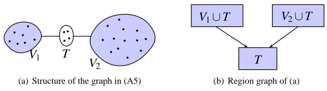
(A6) Structure of G∗: Under (A3), we assume that there exists a set of vertices V
1, V2,
and T such that T separates V1 and V2 in G∗ and |T| < η. Figure 8(a) shows the
general structure of this assumption.
Assumptions (A1)-(A5) are standard conditions for proving high-dimensional consis-tency of the PC-Algorithm for Gaussian graphical models. The structural constraints on
Vats and Nowak
Journal of Machine Learning Research () Submitted 4/13; Revised 9/13; Published
-T
V
1V
2(a) Structure of the graph in (A5)
V
1∪
T
V
2∪
T
T
(b) Region graph of (a)
c
Divyanshu Vats and Robert D. Nowak.
Figure 8: General Structure of the graph we use in showing the advantages of the junction tree framework.
the graph in Assumption (A6) are required for showing the advantages of the junction tree framework. We note that although (A6) appears to be a strong assumption, there are several graph families that satisfy this assumption. For example, the graph in Figure 1(a) satisfies (A6) with V1 = {1,2}, V2 = {1,3,4,5,6,7}, and T = {1}. In general, if there
exists a separator in the graph of size less than η, then (A6) is clearly satisfied. Further, we remark that we only assume the existence of the sets V1,V2, and T and do not assume
that these sets are knowna priori. We refer to Remark 17 for more discussions about (A6) and some extensions of this assumption.
7.2 Theoretical Result and Analysis
RecallPC in Algorithm 4. Since we assume (A1), the conditional independence test in (4) can be used in Line 5 of Algorithm 4. To analyze the junction tree framework, consider the following steps to constructGb using PC when givenni.i.d. observations Xn:
Step 1. ComputeH: Apply PCusing a regularization parameter λ0
n such that
H=PC(|T|,Xn, KV, KV),
whereKV is the complete graph over the nodesV. In the above equation, we apply PC to remove all edges for which there exists a separator of size less than or equal to|T|.
Step 2. Estimate a subset of edges overV1∪T and V2∪T using regularization parameters
λ1
n andλ2n, respectively, such that
b
GVk =PC η,X n, H[V
k∪T]∪KT, HV0k∪T
,fork= 1,2,
whereHV0
k∪T =H[Vk∪T]\KT as defined in (3).
Step 3. Estimate edges overT using a regularization parameterλT n:
b
GT =PC
η,Xn, H[T∪ne b
GV1∪GbV2(T)], H[T]
.
Step 4. Final estimate is Gb=GbV1∪GbV2 ∪GbT.
A Junction Tree Framework for Undirected Graphical Model Selection
Step 1 is the screening algorithm used to eliminate some edges from the complete graph. For the region graph in Figure 8(b), Step 2 corresponds to applyingPCto the regionsV1∪T
and V2 ∪T. Step 3 corresponds to applying PC to the region T and all neighbors of T
estimated so far. Step 4 merges all the estimated edges. Although the neighbors of T are sufficient to estimate all the edges in T, in general, depending on the graph, a smaller set of vertices is required to estimate edges inT. The main result is stated using the following terms defined on the graphical model:
p1 =|V1|+|T|, p2=|V2|+|T|, pT =|T ∪neG∗(T)|, ηT =|T|,
ρ0 = inf{|ρij|S|:i, j s.t.|S| ≤ηT &|ρij|S|>0},
ρ1 = inf{|ρij|S|:i∈V1, j∈V1∪T s.t.(i, j)∈E(G∗), S ⊆V1∪T,|S| ≤η},
ρ2 = inf{|ρij|S|:i∈V2, j∈V2∪T s.t.(i, j)∈E(G∗), S ⊆V2∪T,|S| ≤η},
ρT = inf{|ρij|S|:i, j∈T s.t.(i, j)∈E, S ⊆T∪neG∗(T), ηT <|S| ≤η},
The termρ0 is a measure of how hard it is to learn the graphH in Step 1 so thatE(G∗)⊆
E(H) and all edges that have a separator of size less than|T|are deleted inH. The termsρ1
andρ2 are measures of how hard it is learn the edges inG∗[V1∪T]\KT and G∗[V2∪T]\KT
(Step 2), respectively, given that E(G∗) ⊆E(H). The term ρT is a measure of how hard
it is learn the graph over the nodesT given that we know the edges that connect V1 toT
and V2 toT.
Theorem 9 Under Assumptions (A1)-(A6), there exists a conditional independence test such that if
n= Ω maxρ−02ηTlog(p), ρ−12ηlog(p1), ρ2−2ηlog(p2), ρT−2ηlog(pT) , (7)
thenP(Gb6=G)→0 as n→ ∞.
Proof See Appendix E.
We now make several remarks regarding Theorem 9 and its consequences.
Remark 10 (Comparison to Necessary Conditions) Using results from Wang et al. (2010), it follows that a necessary condition for any algorithm to recover the graphG∗ that satisfies Assumptions (A1) and (A6) is that n= Ω(max{θ−2
1 log(p1 −d), θ2−2log(p2 −d)},
wheredis the maximum degree of the graph andθ1 andθ2 are defined as follows:
θk = min
(i,j)∈G∗[V
k∪T]\G∗[T]
|Σ−ij1|
q
|Σ−ii1Σ−jj1|
, k= 1,2.
Ifηis a constant andρ1andρ2are chosen so that the corresponding expressions dominate all
other expressions, then (7) reduces to n= Ω(max{ρ−12log(p1), ρ−22log(p2)}). Furthermore,
for certain classes of Gaussian graphical models, namely walk summable graphical models (Malioutov et al., 2006), the results in Anandkumar et al. (2012a) show that there exists conditions under which ρ1 = Ω(θ1) and ρ2 = Ω(θ2). In this case, (7) is equivalent to
Vats and Nowak
of graphical models for which the sufficient conditions in Theorem 9 nearly match the necessary conditions for asymptotically reliable estimation of the graph. We note that the particular family of graphical models is quite broad, and includes forests, scale-free graphs, and some random graphs. We refer to Anandkumar et al. (2012a) for a characterization of such graphical models.
Remark 11 (Choice of Regularization Parameters)We use the conditional indepen-dence test in (4) that thresholds the conditional correlation coefficient. From the proof in Appendix E, the thresholds, which we refer to as the regularization parameter, are chosen as follows:
λ0n=O(ρ0) and ρ0 = Ω p
ηT log(p)/n
,
λk
n=O(ρk) andρk= Ω
p
ηlog(pk)/n
, k= 1,2,
λTn =O(ρT) and ρT = Ω
p
ηlog(pT)/n
.
We clearly see that different regularization parameters are used to estimate different parts of the graph. Furthermore, just like in the traditional analysis of UGMS algorithms, the optimal choice of the regularization parameter depends on unknown parameters of the graphical model. In practice, we use model selection algorithms to select regularization parameters. We refer to Section 8 for more details.
Remark 12 (Weaker Condition) If we do not use the junction tree based approach outlined in Steps 1-4, and instead directly applyPC, the sufficient condition on the number of observations will ben= Ω(ρ−min2 ηlog(p)), where
ρmin:= inf{|ρij|S|: (i, j)∈E(G∗),|S| ≤η}.
This result is proved in Appendix D using results from Kalisch and B¨uhlmann (2007) and Anandkumar et al. (2012a). Sinceρmin≤min{ρ0, ρ1, ρ2, ρT}, it is clear that (7) is a weaker
condition. The main reason for this difference is that the junction tree approach defines an ordering on the edges to test if an edge belongs to the true graph. This ordering allows for a reduction in separator search space (seeSij in Algorithm 4) for testing edges over the set
T. Standard analysis ofPCassumes that the edges are tested randomly, in which case, the separator search space is always upper bounded by the full set of nodes.
Remark 13 (Reduced Sample Complexity) Supposeη,ρ0, and ρT are constants and
ρ1 < ρ2. In this case, (7) reduces to
n= Ω maxlog(p), ρ−12log(p1), ρ−22log(p2) . (8)
Ifρ−12= Ω maxρ−22log(p2)/log(p1),log(p) , then (8) reduces to
n= Ω ρ−12log(p1)
.
On the other hand, if we do not use junction trees, n = Ω ρ−min2 log(p), where ρmin ≤
ρ1. Thus, if p1 p, for example p1 = log(p), then using the junction tree based PC
A Junction Tree Framework for Undirected Graphical Model Selection
Journal of Machine Learning Research () Submitted 4/13; Revised 9/13; Published
-V
2V
1V
3V
4V
5V
1∪
5i=2
V
ic
Divyanshu Vats and Robert D. Nowak.
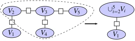
Figure 9: Junction tree representation with clusters V1, . . . , V5 and separators denotes by
rectangular boxes. We can cluster vertices in the junction tree to get a two cluster representation as in Figure 8.
requires lower number of observations for consistent UGMS. Informally, the above condition says that if the graph structure in (A6) is easy to identify, p1 p2, and the minimal
conditional correlation coefficient over the true edges lies in the smaller cluster (but not over the separator), the junction tree framework may accurately learn the graph using significantly less number of observations.
Remark 14 (Learning Weak Edges)We now analyze Theorem 9 to see how the condi-tional correlation coefficients scale for high-dimensional consistency. Under the assumption in Remark 13, it is easy to see that the minimal conditional correlation coefficient scales as Ω(plog(p1)/n) when using junction trees and as Ω(
p
log(p)/n) when not using junction trees. This suggests that when p1 p, it may be possible to learn edges with weaker
conditional correlation coefficients when using junction trees. Our numerical simulations in Section 8 empirically show this property of the junction tree framework.
Remark 15 (Computational complexity)It is easy to see that the worst case compu-tational complexity of the PC-Algorithm isO(pη+2) since there areO(p2) edges and testing
for each edge requires a search over at mostO(pη) separators. The worst case computational
complexity of Steps 1-4 is roughly Op|T|+2+pη+2 1 +p
η+2 2 +p
η+2 T
. Under the conditions in Remark 8.3 and when p1 p, this complexity is roughly O(pη+2), which is the same as
the standard PC-Algorithm. In practice, especially when the graph is sparse, the compu-tational complexity is much less thanO(pη+2) since the PC-Algorithm restricts the search
space for finding separators.
Remark 16 (Using other UGMS Algorithms) Although our analysis used the
PC-Algorithm to derive sufficient conditions for accurately estimating the graph, we can easily use other algorithms, such as the graphical Lasso or the neighborhood selection based Lasso, for analysis. The main difference will be in the assumptions imposed on the graphical model.
Vats and Nowak
the structure in Figure 8. For example, suppose the graph G∗ has a junction tree repre-sentation as in Figure 9 with five clusters. If |V1∩V2|< η, then we can merge the clusters
V2, V3, . . . , V5 so that the resulting junction tree admits the two cluster representation in
Figure 8. Furthermore, we can also generalize Theorem 9 to cases when|T|=η. The main change in the analysis will be in the definition ofρ0. For example, if the graph is a chain so
that the first p1 vertices are associated with “weak edges”, we can get similar results as in
Theorem 9. Finally, we note that a full analysis of the junction tree framework, that also incorporates the step of updating the junction tree in Algorithm 3, is challenging and will be addressed in future work.
8. Numerical Simulations
In this section, we present numerical simulations that highlight the advantages of using the junction tree framework for UGMS. Throughout this section, we assume a Gaussian graphical model such that PX ∼ N(0,Θ−1) is Markov on G∗. It is well known that this
implies that (i, j) ∈/ G∗ ⇐⇒ Θij = 0 (Speed and Kiiveri, 1986). Some algorithmic details
used in the simulations are described as follows.
Computing H: We apply Algorithm 4 with a suitable value of κ in such a way that the separator search space Sij (see Line 4) is restricted to be small. In other words, we do
not test for all possible conditional independence tests so as to restrict the computational complexity of the screening algorithm. We use the conditional partial correlation to test for conditional independence and choose a separate threshold to test for each edge in the graph. The thresholds for the conditional independence test are computed using 5-fold cross-validation. The computational complexity of this step is roughly O(p2) since there
areO(p2) edges to be tested. Note that this method for computingHis equivalent to Step 1
in Section 7.2 with |T| = κ. Finally, we note that the above method does not guarantee that all edges in G∗ will be included in H. This can result in false edges being included in the junction tree estimated graphs. To avoid this situation, once a graph estimate Gb has been computed using the junction tree based UGMS algorithm, we apply conditional independence tests again to prune the estimated edge set.
Computing the junction tree: We use standard algorithms in the literature for computing close to optimal junction trees.4 Once the junction tree is computed, we merge clusters so
that the maximum size of the separator is at most κ+ 1, where κ is the parameter used when computing the graphH. For example, in Figure 9, if the separator associated withV2
and V3 has cardinality greater thanκ+ 1, then we merge V2 andV3 and resulting junction
tree is such that V1,V4, and V5 all connect to the cluster V2∪V3.
UGMS Algorithms: We apply the junction tree framework in conjunction with graphical Lasso (gL) (Banerjee et al., 2008), neighborhood selection using Lasso (nL) (Meinshausen and B¨uhlmann, 2006), and the PC-Algorithm (PC) (Spirtes and Glymour, 1991). See Appendix B for a review ofgLand nL and Algorithm 4 forPC. When usingnL, we use the intersection rule to combine neighborhood estimates. Further, we use the adaptive Lasso (Zou, 2006) for finding neighbors of a vertex since this is known to give superior results for variable selection (van de Geer et al., 2011).
4. We use the GreedyFillin heuristic. This is known to give good results with reasonable computational time (Kjaerulff, 1990).
A Junction Tree Framework for Undirected Graphical Model Selection
Choosing Regularization Parameters: An important step when applying UGMS algorithms is to choose a suitable regularization parameter. It is now well known that classical methods, such as cross-validation and information criterion based methods, tend to choose a much larger number of edges when compared to an oracle estimator for high-dimensional problems (Meinshausen and B¨uhlmann, 2010; Liu et al., 2010). Several alternative methods have been proposed in the literature; see for example stability selection (Meinshausen and B¨uhlmann, 2010; Liu et al., 2010) and extended Bayesian information (EBIC) criterion (Chen and Chen, 2008; Foygel and Drton, 2010). In all our simulations, we use EBIC since it is much faster than stability based methods when the distribution is Gaussian. EBIC selects a regularization parameterbλnas follows:
b
λn= max λn>0
n
nhlog detΘbλn−trace(SbΘ) i
+|E(Gbλn)|logn+ 4γ|E(Gbλn)|logp o
,
where Sb is the empirical covariance matrix, Θbλn is the estimate of the inverse covariance
matrix and |E(Gbλn)| is the number of edges in the estimated graph. The estimate bλn
depends on a parameterγ ∈[0,1] such thatγ = 0 results in the BIC estimate and increasing γ produces sparser graphs. The authors in reference Foygel and Drton (2010) suggest that γ = 0.5 is a reasonable choice for high-dimensional problems. When solving subproblems using Algorithm 2, the logp term is replaced by log|R|, Θbλn is replaced by the inverse
covariance over the verticesR, and|Gbλn|is replaced by the number of edges estimated from
the graph HR0 .
Small subproblems: Whenever|R|is small (less than 8 in our simulations), we independently test whether each edge is inG∗ using hypothesis testing. This shows the application of using different algorithms to learn different parts of the graph.
8.1 Results on Synthetic Graphs
We assume that Θii = 1 for alli= 1, . . . , p. We refer to all edges connected to the first p1
vertices asweak edges and the rest of the edges are referred to asstrong edges. The different types of synthetic graphical models we study are described as follows:
• Chain (CH1 and CH2): Θi,i+1 =ρ1 fori= 1, . . . , p1−1 (weak edges) and Θi,i+1=ρ2
for i = p1, p−1 (strong edges). For CH1, ρ1 = 0.15 and ρ2 = 0.245. For CH2, ρ1 = 0.075 and ρ2 = 0.245. Let Θij = Θji.
• Cycle (CY1 and CY2): Θi,i+1 =ρ1 fori= 1, . . . , p1−1 (weak edges) and Θi,i+1 =ρ2
for i = p1, p−1 (strong edges). In addition, Θi,i+3 = ρ1 for i = 1, . . . , p1 −3 and
Θi,i+3=ρ2 fori=p1, p1+ 1, . . . , p−3. This introduces multiple cycles in the graph.
ForCY1,ρ1 = 0.15 andρ2 = 0.245. ForCY2,ρ1 = 0.075 and ρ2 = 0.245.
• Hub (HB1 and HB2): For the firstp1 vertices, construct as many star5 graphs of size
d1 as possible. For the remaining vertices, construct star graphs of size d2 (at most
one may be of size less thand2). The hub graph G∗ is constructed by taking a union
of all star graphs. For (i, j) ∈ G∗ s.t. i, j ≤ p1, let Θi,j = 1/d1. For the remaining
edges, let Θij = 1/d2. ForHB1,d1= 8 and d2 = 5. For HB2,d1= 12 and d2 = 5.
Vats and Nowak
• Neighborhood graph (NB1 and NB2): Randomly place vertices on the unit square at coordinates y1, . . . , yp. Let Θij = 1/ρ1 with probability (
√
2π)−1exp(−4||y
i −yj||22),
otherwise Θij = 0 for alli, j∈ {1, . . . , p1}such thati > j. For alli, j∈ {p1+ 1, . . . , p}
such thati > j, Θij =ρ2. For edges over the firstp1 vertices, delete edges so that each
vertex is connected to at mostd1 other vertices. For the vertices p1+ 1, . . . , p, delete
edges such that the neighborhood of each vertex is at mostd2. Finally, randomly add
four edges from a vertex in {1, . . . , p1}to a vertex in {p1, p1+ 1, . . . , p} such that for
each such edge, Θij =ρ1. We let ρ2 = 0.245, d1 = 6, andd2 = 4. For NB1,ρ1 = 0.15
and for NB2,ρ2= 0.075.
Notice that the parameters associated with the weak edges are lower than the parameters associated with the strong edges. Some comments regarding notation and usage of various algorithms is given as follows.
• The junction tree versions of the UGMS algorithms are denoted by JgL, JPC, and
JnL.
• We use EBIC with γ = 0.5 to choose regularization parameters when estimating graphs using JgLand JPC. To objectively compare JgL(JPC) andgL (PC), we make sure that the number of edges estimated bygL(PC) is roughly the same as the number of edges estimated by JgL(JPC).
• The nL and JnL estimates are computed differently since it is difficult to control the number of edges estimated using both these algorithms.6 We apply bothnL and JnL
for multiple different values ofγ (the parameter for EBIC) and choose graphs so that the number of edges estimated is closest to the number of edges estimated by gL.
• When applyingPCandJPC, we chooseκ as 1, 2, 1, and 3 for Chain, Cycle, Hub, and Neighborhood graphs, respectively. When computing H, we choose κ as 0, 1, 0, and 2 for Chain, Cycle, Hub, and Neighborhood graphs, respectively.
Tables 2-5 summarize the results for the different types of synthetic graphical models. For an estimateGb ofG∗, we evaluate Gb using the weak edge discovery rate (WEDR), false discovery rate (FDR), true positive rate (TPR), and the edit distance (ED).
WEDR = # weak edges in Gb
# of weak edges inG∗ ,
FDR = # of edges in Gb\G ∗
# of edges in Gb ,
TPR = # of edges in Gb∩G ∗
# of edges inG∗ ,
ED ={# edges in Gb\G∗}+{# edges in G∗\Gb},
6. Recall that both these algorithms use different regularization parameters. Thus, there may exist multiple different estimates with the same number of edges.