Iterative and Active Graph Clustering Using Trace Norm
Minimization Without Cluster Size Constraints
∗Nir Ailon [email protected]
Department of Computer Science Technion IIT Haifa, Israel
Yudong Chen [email protected]
Department of Electrical Engineering and Computer Sciences University of California, Berkeley
Berkeley, CA 94720, USA
Huan Xu [email protected]
Department of Mechanical Engineering National University of Singapore Singapore 117575
Editor:Tong Zhang
Abstract
This paper investigates graph clustering under the planted partition model in the presence of small clusters. Traditional results dictate that for an algorithm to provably correctly recover the underlying clusters, all clusters must be sufficiently large—in particular, the cluster sizes need to be ˜Ω(√n), where n is the number of nodes of the graph. We show that this is not really a restriction: by a refined analysis of a convex-optimization-based recovery approach, we prove that small clusters, under certain mild assumptions, do not hinder recovery of large ones. Based on this result, we further devise an iterative algorithm to provably recover almost all clustersvia a “peeling strategy”: we recover large clusters first, leading to a reduced problem, and repeat this procedure. These results are extended to the partial observation setting, in which only a (chosen) part of the graph is observed. The peeling strategy gives rise to an active learning algorithm, in which edges adjacent to smaller clusters are queried more often after large clusters are learned (and removed). We expect that the idea of iterative peeling—that is, sequentially identifying a subset of the clusters and reducing the problem to a smaller one—is useful more broadly beyond the specific implementations (based on convex optimization) used in this paper.
Keywords: graph clustering, community detection, active clustering, convex optimiza-tion, planted partition model, stochastic block model
1. Introduction
This paper considers the following classic graph clustering problem: given an undirected unweighted graph, partition the nodes into disjoint clusters so that the density of edges within each cluster is higher than those across clusters. Graph clustering arises naturally in many applications across science and engineering; prominent examples include community
detection in social networks (Mishra et al., 2007; Zhao et al., 2011), submarket identification in E-commerce and sponsored search (Yahoo!-Inc, 2009), and co-authorship analysis in document database (Ester et al., 1995), among others. From a purely binary classification theoretical point of view, the edges of the graph are (noisy) labels of “similarity” or “affinity” between pairs of objects, and the concept class consists of clusterings of the objects (encoded graphically by identifying clusters with cliques).
Many theoretical results in graph clustering consider thePlanted Partition Model (Con-don and Karp, 2001), in which the edges are generated randomly based on an unknown set of underlying clusters; see Section 1.1 for more details. While numerous different meth-ods have been proposed, their performance guarantees under the planted partition model generally have the following form: under certain conditions of the density of edges (within clusters and across clusters), the method succeeds to recover the correct clusters exactly if all clusters are larger than a threshold size, typically ˜Ω(√n);1 see e.g., McSherry (2001); Bollob´as and Scott (2004); Ames and Vavasis (2011); Chen et al. (2012); Chaudhuri et al. (2012); Anandkumar et al. (2014).
In this paper, we aim to relax this cluster size constraint of graph clustering under the planted partition model. Identifying extremely small clusters is inherently hard as they are easily confused with “fake” clusters generated by noisy edges,2 and is not the focus of this paper. Instead, in this paper we investigate a question that has not been addressed before: Can we still recover large clusters in the presence of small clusters? Intuitively, this should be doable. To illustrate, consider an extreme example where the given graphG consists of two subgraphs G1 and G2 with disjoint node sets. SupposeG1, if presented alone, can be
correctly clustered using some existing methods, G2 is a very small clique, and there are
relatively few edges connecting G1 and G2. The graph G certainly violates the minimum
cluster size requirement of previous results, but why shouldG2 spoil our ability to correctly
cluster G1?
Our main result confirms this intuition. We show that the cluster size barrier arising in previous work is not really a restriction, but rather an artifact of the attempt to solve the problem in a single shot and recover large and small clusters simultaneously. Using a more careful analysis, we prove that a mixed trace-norm and `1-norm based convex formulation
can recover clusters of size ˜Ω(√n) even in the presence of smaller clusters. That is, small clusters do not interfere with recovery of the large clusters.
The main implication of this result is that one can apply aniterative “peeling” strategy
to recover smaller and smaller clusters. The intuition is simple: suppose the number of
clusters is limited, then either all clusters are large, or the sizes of the clusters vary signif-icantly. The first case is obviously easy. But the second is also tractable, for a different reason: using the aforementioned convex formulation, the larger clusters can be correctly identified; if we remove all nodes from these larger clusters, the remaining subgraph contains significantly fewer nodes than the original graph, which leads to a much lower threshold on the size of the cluster for correct recovery, making it possible for correctly identify some
1. The notations ˜Ω(·) and ˜O(·) ignore logarithmic factors.
smaller clusters. By repeating this procedure, indeed, we can recover the cluster structure for almost all nodes with no lower bound on the minimal cluster size. Below we summarize our main contributions and techniques:
1. We provide a refined analysis (Theorem 2) of the mixed trace-norm and `1-norm
convex relaxation approach for exact cluster recovery proposed in Chen et al. (2014a, 2012), focusing on the case where small clusters exist. We show that in the planted partition setting, if each cluster is either large (more precisely, of size at leastσ ≈√n)
or small (of size at most σ/C for some global constant C > 1), then with high
probability, this convex relaxation approach correctly identifies all large clusters while “ignoring” the small ones. In fact, it is possible to arbitrarily increase the tuning parameter σ in quest of an interval (σ/C, σ) that is disjoint from the set of cluster sizes. The analysis is done by identifying a certain feasible solution to the convex program and proving its almost sure optimality. This solution easily identifies the large clusters. Previous analysis is performed only in the case where all clusters are of size greater than√n.
2. We provide a converse (Theorem 5) of the result just described. More precisely, we
show that if for some value of the tuning parameter σ, an optimal solution to the
convex relaxation program is an exact representation of a collection of large clusters (a partial clustering), then these clusters are actual ground truth clusters, even if the particular interval corresponding to σ isn’t really free of cluster sizes. This allows
the practitioner to be certain that the optimal solution is useful. Moreover, this
has important algorithmic implications for an iterative recovery procedure which we describe below.
3. The last two points imply that if some interval of the form (σ/C, σ) is free of cluster sizes, then an exhaustive search of this interval will constructively find large clusters, though not necessarily for that particular interval (Theorem 6). Removing the re-covered large clusters leads to a reduced problem with a smaller graph. Repeating this procedure gives rise to an iterative algorithm (Algorithm 2), using a “peeling strategy”, to recover smaller and smaller clusters that are otherwise impossible to re-cover. Using this iterative algorithm, we prove that as long as the number of clusters is bounded by O(logn), regardless of the cluster sizes, we can correctly recover the cluster structure for an overwhelming fraction of nodes (Theorem 7). To the best of our knowledge, this is the first result of provably correct graph clustering assuming only an upper bound on the number of clusters, but otherwise no assumption on the cluster sizes.
guarantees are given for this algorithm (Corollary 8–Theorem 11). This active learning scheme requires significantly fewer samples than uniform sampling .
Beside these technical contributions, this paper suggests a new strategy that is poten-tially useful for general low-rank matrix recovery and other high-dimensional statistical problems, where the data are typically assumed to have certain low-dimensional structures. Many methods have been developed to exploit this a priori structural information so that consistent estimation is possible even when the dimensionality of the problem is larger than the number of samples. Our result shows that one may combine these methods with a “peeling strategy” to further push the envelope of learning structured data: by iteratively recovering the easier structural components and reducing the problem complexity, it may be possible to learn complicated structures that are otherwise difficult to recover using existing one-shot approaches.
1.1 Related Work
The literature of graph clustering is too vast for a detailed survey here; we concentrate on the most related work, and in particular those provide provable guarantees on exact cluster recovery.
1.1.1 Planted Partition Model
Also known as the stochastic block model (Holland et al., 1983; Condon and Karp, 2001),
this classical model assumes that n nodes are partitioned into subsets, referred to as the “true clusters”, and a graph is randomly generated as follows: for each pair of nodes, de-pending on whether or not they belong to the same subset, an edge connecting them is generated with a probability p or q respectively. The goal is to correctly recover the clus-ters given the random graph. The planted partition model has a large body of literature. Earlier work focused on the setting where the minimal cluster size is Θ(n) (Boppana, 1987;
Condon and Karp, 2001; Carson and Impagliazzo, 2001; Bollob´as and Scott, 2004).
1.1.2 Low-rank and Sparse Matrix Decomposition via Trace Norm
Motivated by robustifying principal component analysis (PCA), several authors (Chan-drasekaran et al., 2011; Cand`es et al., 2011) show that it is possible to recover a low-rank matrix from sparse errors of arbitrary magnitude, where the key ingredient is using the trace norm (also known as the nuclear norm) as a convex surrogate of the rank. Similar results are obtained when the low rank matrix is corrupted by other types of noise (Xu et al., 2012). Of particular relevance to this paper is the work by Jalali et al. (2011), Oymak and Hassibi (2011) and Chen et al. (2012, 2014a), where they apply this approach to graph clustering, and specifically to the planted partition model. These works require the ˜Ω(√n) bound on the minimal cluster size. Our approach uses the trace norm relaxation, combined with a more refined analysis and an iterative/active peeling strategy.
1.1.3 Active Learning/Active Clustering
Another line of work that motivates this paper is the study of active learning (a setting in which labeled instances are chosen by the learner, rather than by nature), and in particular active learning algorithms for clustering. The most related work is Ailon et al. (2014), who investigated active learning for the correlation clustering problem (Bansal et al., 2004), where the goal is to find a set of clusters whose Hamming distance from the graph is minimized. Ailon et al. (2014) obtain a (1 +ε)-approximate solution with respect to the optimum, while (actively) querying no more than O(npoly(logn, k, ε−1)) edges, where k
is the number of clusters. Their result imposed no restriction on cluster sizes and hence inspired this work, but differs in at least two major ways. First, Ailon et al. (2014) did not considerexact cluster recovery as we do. Second, their guarantees fall in the Empirical
Risk Minimization (ERM) framework, with no running time guarantees. Our work uses a
convex relaxation algorithm, and is hence computationally efficient. The problem of active learning has also been investigated in other setups including clustering based on distance matrix (Voevodski et al., 2012; Shamir and Tishby, 2011), hierarchical clustering (Eriksson et al., 2011; Krishnamurthy et al., 2012) and low-rank matrix/tensor recovery (Krishna-murthy and Singh, 2013). These setups differ significantly from ours..
Remark 1 (A note on a preliminary version of this paper) The authors published a weaker version of the results in this paper in a preliminary conference paper (Ailon et al., 2013). An exact comparison is stated after each theorem in the text.
2. Notation and Setup
In this paper the following notations are used. We use X(i, j) to denote the (i, j)-the entry of a matrix X. For a matrixX ∈Rn×n and a subset S ⊆[n] of size m, the matrix X[S] ∈ Rm×m is the principal minor of X corresponding to the set of indexes S. For a
matrix M, s(M) denotes the support of M, namely, the set of index pairs (i, j) such that
M(i, j)6= 0. For any subset Φ of [n]×[n], PΦM is the matrix that satisfies
(PΦM)(i, j) = (
M(i, j), (i, j)∈Φ
We now describe the problem setup. Throughout the paper, V denotes a ground set of elements, which we identify with the set [n] = {1, . . . , n}. We assume a ground truth clustering of V given by a pairwise disjoint covering V1, . . . , Vk, where k is the number of
clusters. We say i∼ j if i, j ∈Va for some a∈[k], otherwise i6∼j. We letna := |Va|be
the size of the a-th cluster for each a∈[k]. For each i∈[n],hii is index of the cluster that containsi, the unique index satisfyingi∈Vhii.
The ground truth clustering matrix, denoted as K∗, is defined as the n×nmatrix so thatK∗(i, j) = 1 ifi∼j, otherwise 0. This is a block diagonal matrix, each block consisting of 1’s only, and its rank is k. The input is a symmetric n×n matrix A, which is a noisy version of K∗. It is generated according to the planted partition model with parameters p
and q as follows.
We think of A as the adjacency matrix of an undirected random graph, where
the edge (i, j) is in the graph fori > j with probability pij if i∼j, otherwise
with probability qij, independent of other choices, where we only assume the edge probabilities satisfy (minpij) =:p > q := (maxqij).
We use the convention that the diagonal entries of A are all 1. The matrix B∗ :=A−K∗
can be viewed as the noise matrix. GivenA, the task is to find the ground truth clusters. We remark that the setup above is more flexible than the standard planted partition model: we allow the clusters to have different sizes, and the edges probabilities (pij andqij)
need not be uniform across node pairs (i, j). One consequence is that the node degrees may not be uniform or correlated with the sizes of the associated clusters. Non-uniformity makes some simple heuristics, such as degree counting and single linkage clustering, vulnerable. For example, we cannot distinguish between large and small clusters simply by looking at the node degrees, since nodes in a small cluster may also have high expected degrees. The single linkage clustering approach also fails in the presence of non-uniformity. We illustrate this with an example. Suppose there are √n clusters of equal size, p= 1 andq = 0.1. We use the number of common neighbors as the distance function in single linkage clustering. If allqij are equal toq, then it is easy to see that single linkage clustering will succeed, since
with high probability node pairs in the same cluster will have more common neighbors than those in different clusters. Yet, this is not true for non-uniformqij’s. Consider three nodes 1, 2 and 3, where nodes 1 and 2 are in the same cluster, and node 3 belongs to a different cluster. Suppose for all i > 3, q1i = 0, q2i =q3i = 0.1. The expected number of common
neighbors between nodes 1 and 2 is√n, whereas the expected number of common neighbors between nodes 2 and 3 is 0.2√n+ 0.01(n−2√n), which is larger than √nfor largen and hence single linkage clustering fails. In contrast, the proposed convex-optimization based method can handle such non-uniform settings, as we show in what follows.
3. Main Results
We remind the reader that the trace norm of a matrix is the sum of its singular values, and the (entry-wise) `1 norm of a matrix M iskMk1 :=Pi,j|M(i, j)|. Consider the following
another matrix variable B using two parameters c1, c2 that will be determined later:
(CP) min
K,B∈Rn×n
kKk∗+c1 Ps(A)B
1+c2
Ps(A)cB 1
s.t. K+B=A,
0≤Kij ≤1,∀(i, j).
Here the trace norm term in the objective promotes low-rank solutions and thus encourages
the matrix K to have the zero-one block-diagonal structure of a clustering matrix. The
matrix Ps(A)B =Ps(A)(A−K) is non-zero only on the pairs (i, j) between which there is an edge in the graph (Aij = 1) but the candidate solution has Kij = 0, and thus Ps(A)B
corresponds to the “cross-cluster disagreements” between A and K. Similarly, the matrix
Ps(A)cB corresponds to the “in-cluster disagreements”. Hence, the last two terms in the
objective is the weighted sum of these two types of disagreements. The formulation (CP) can therefore be considered as a convex relaxation of the so-calledweighted correlation clustering
approach (Bansal et al., 2004), whose objective is to find a clustering that minimizes the weighted disagreements. See Oymak and Hassibi (2011); Mathieu and Schudy (2010); Chen et al. (2014a) for related formulations.
Important to subsequent development is the following new theoretical guarantee for the formulation (CP). We show that (CP) identifies the large clusters whose sizes are above a threshold (chosen by the user) even when small clusters are present. The proof is given in Section 5.1.
Theorem 2 There exist universal constants b3 > 1 > b4 > 0 such that the following is
true. For any (user-specified) parametersκ≥1 andt∈[14p+34q,34p+14q], define
`] :=b3
κpp(1−q)n
p−q max
(
1,
p
p(1−q) log4n κ(p−q)√n
)
, `[:=b4
κpp(1−q)n
p−q , (1)
and set
c1 :=
1 100κ√n
r
1−t
t , c2 :=
1 100κ√n
r
t
1−t . (2)
If (i) n≥ `] and n ≥700, and (ii) for each a∈ [k], either na ≥ `] or na ≤`[, then with probability at least 1−n−3, the optimal solution to (CP) with c1, c2 given above is unique
and equal to( ˆK,Bˆ) = (P]K∗, A−Kˆ), where for a matrix M, P]M is the matrix defined by
(P]M)(i, j) =
(
M(i, j), max{nhii, nhji} ≥`]
0, otherwise.
The theorem improves on a weaker version in Ailon et al. 2013, where the ratio `]/`[ was
larger by a factor of log2nthan here. The theorem says that the solution to (CP) identifies clusters of size larger than `]= Ω(κ
√
Black represents 1, white represents 0. Here
σmin(K) is the side length of the smallest
black square.
Figure 1: Illustration of a partial clustering matrixK.
Note that by the theorem’s premise, ˆK is the matrix obtained fromK∗ after zeroing out blocks corresponding to clusters of size at most `[. Also note that under the assumption
p−q≥pp(1−q) log4n/√n , (3)
we get the following simpler expression for`] in the theorem, replacing its definition in (1):
`] =b3
κpp(1−q)n
p−q . (4)
In this case,`]and `[ differ by only a multiplicative absolute constantb3/b4. We will make
the assumption (3) in what follows for simplicity, although it is not generally necessary.
Remark 3 The requirement of having a multiplicative constant gapb3/b4 between the sizes
`] and`[ of the large and small clusters, is not an artifact of our analysis; cf. the discussion at the end of Section 4.
For the convenience of subsequent discussion, we use the following definition.
Definition 4 (Partial Clustering Matrix) An n×n matrix K is said to be a partial clustering matrix if there exists a collection of pairwise disjoint sets U1, . . . , Ur ⊆V (called the induced clusters) such thatK(i, j) = 1if and only ifi, j∈Ua for somea∈[r], otherwise
0. If K is a partial clustering matrix then σmin(K) is defined asmina∈[r]|Ua|.
The definition is depicted in Figure 1. The key message in Theorem 2 is that by choosingκ
properly such that no cluster size falls in the interval (`[, `]), the unique optimal solution
( ˆK,Bˆ) to the convex program (CP) is such that ˆK is a partial clustering corresponding to large ground truth clusters.
But how can we choose a properκ? Moreover, given that we chose aκ(say, by exhaustive search), how can we certify that it was indeed chosen properly? In order to develop an algorithm, we would need a type of converse of Theorem 2: There exists an event with high probability (in the random process generating the input graph), such that conditioned on this event, for all values of κ, if an optimal solution to the corresponding (CP) is a partial clustering matrix with the structure illustrated in Figure 1, then the blocks of ˆKcorrespond to ground truth clusters.
Theorem 5 There exist absolute constants C1, C2 > 0 such that with probability at least
an optimal solution to (CP) with c1, c2 as defined in Theorem 2, and additionally K is a
partial clustering corresponding to U1, . . . , Ur⊆V, with
σmin(K)≥max (
C1klogn
(p−q)2 ,
C2κ p
p(1−q)nlogn p−q
)
, (5)
thenU1, . . . , Ur are actual ground truth clusters, namely, there exists an injectionφ: [r]7→
[k]such that Ua=Vφ(a) for all a∈[r]. Algorithm 1 RecoverBigFullObs(V, A, p, q)
require: ground setV, graph A∈RV×V, probabilities p, q n← |V|
t← 14p+34q (or anything in [14p+34q,34p+ 14q])
`]←n,g← bb34
// (If have prior bound k0 on the number of clusters, take `]←n/k0) while `]≥max
C1klogn (p−q)2 ,
C2
√
p(1−q)nlogn p−q
do
solve forκ using (1), setc1, c2 as in (2)
(K, B)←optimal solution to (CP) with c1, c2
if K is a partial clustering matrix with σmin(K)≥`] then
return induced clusters{U1, . . . , Ur} ofK end if
`]←`]/g
end while return ∅
The proof is given in Section 5.2. The combination of Theorems 2 and 5 implies the following, which we state in rough terms for simplicity. Let g := b3/b4. Assume that
we iteratively solve (CP) for κ taking values in some decreasing geometric progression of common ratio g (starting at roughly κ=√n), and halt if the optimal solution is a partial clustering with clusters of size at least`]=`](κ) (see Algorithm 1). Then these clusters are
(extremely likely to be) ground truth clusters. Moreover, if for some κ in the sequence, (i) the interval (`[ = `[(κ), `] =`](κ)) intersects no cluster size, and (ii) there is at least one
cluster at least of size `], then such a halt will (be extremely likely to) occur.
The next question is, when are (i) and (ii) guaranteed? If the number of clusters kis a priori bounded by somek0, then there is at least one cluster of size at leastn/k0 (alluding
to (ii)), and by the pigeonhole principle, any set ofk0+ 1 pairwise disjoint intervals of the
form (α, gα) contains at least one interval that intersects no clusters size (alluding to (i)). For simplicity, we make an exact quantification of this principle for the case in which p, q
are assumed to be fixed and independent of n.3 As the following theorem shows, it turns out that in this regime,k0 can be assumed to be asymptotically logarithmic inn to ensure
recovery of at least one cluster.4 In what follows, notation such asC(p, q), C3(p, q) denotes
positive functions that depend onp, q only.
3. In fact, we need only fix (p−q), but we wish to keep this exposition simple.
Algorithm 2 RecoverFullObs(V, A, p, q)
require: ground setV, matrix A∈RV×V, probabilities p, q
{U1, . . . , Ur} ←RecoverBigFullObs(V, A, p, q) V0←[n]\(U1∪ · · · ∪Ur)
if r= 0 then return ∅ else
return RecoverFullObs(V0, A[V0], p, q)∪ {U1, . . . , Ur}
end if
Theorem 6 There exist C3(p, q), C4(p, q), C5 > 0 such that the following holds. Assume
that n > C4(p, q), and that we are guaranteed that k≤k0, where k0 =C3(p, q) logn. Then
with probability at least 1−2n−3, Algorithm 1 will recover at least one cluster in at most C5k0 iterations.
The theorem improves on a counterpart in the preliminary paper (Ailon et al., 2013), where
k0 was smaller by a factor of log lognthan here. Proof Consider the set of intervals
n/(gk0), n/k0
,n/(g2k0), n/(gk0)
, . . . ,n/(gk0+1k
0), n/(gk0k0)
.
By the pigeonhole principle, one of these intervals must not intersect the set of cluster sizes. Assume this interval is (n/(gi0+1k
0), n/(gi0k0)), for some 0 ≤ i0 ≤ k0. By setting
C3(p, q) small enough so thatn/k0is at least Ω( √
nlogn), andC4(p, q) large enough so that
n/gk0+1k
0 is at least Ω( √
nlogn), one easily checks that both the requirements of Theo-rems 2 and 5 are fulfilled.
Theorem 6 ensures that by trying at most a logarithmic number of values of κ, we
can recover at least one large cluster, assuming the number of clusters is logarithmic in n. After recovering and removing such a cluster, we are left with an input of size n0 < n, together with an updated upper bound k00 < k0 on the number of clusters. As long as k00
is logarithmic in n0, we can continue identifying another large cluster (with respect to the smaller problem) using the same procedure. Clearly, as long as the input size is of size at most exp{C3(p, q)k0}, we can iteratively continue this process. The following has been
proved:
Theorem 7 Assume an upper bound k0 on the number k of clusters, and also that n, k0
satisfy the requirements of Theorem 6. Then with probability at least1−2n−2, Algorithm 2 recovers clusters covering all but at most max{exp{C3(p, q)k0}, C4(p, q)} elements, without
any restriction on the minimal cluster size.
The theorem improves on a counterpart in the preliminary paper (Ailon et al., 2013). The consequence is, for example, that if k0 ≤ 2C31(p,q)logn, then the algorithm recovers with
3.1 Partial Observations and Active Sampling
We now consider the case where the input matrixAis not given to us in entirety, but rather that we have oracle access toA(i, j) for (i, j) of our choice. Unobserved values are formally marked asA(i, j) =∗.
Consider a more particular setting in which the edge probabilities arep0 andq0, and the probability of sampling an observation is ρ. More precisely: For i∼j we haveA(i, j) = 1 with probabilityρp0, 0 with probabilityρ(1−p0) and∗with remaining probability, indepen-dently of other pairs. Fori6∼jwe have A(i, j) = 1 with probabilityρq0, 0 with probability
ρ(1−q0) and ∗ with remaining probability, independently of other pairs. Clearly, by pre-tending that the values ∗ in A are 0, we emulate the full observation case of the planted partition model with parameters p=ρp0,q=ρq0.
Of particular interest is the case in which p0, q0 are held fixed andρ tends to zero as n
grows. In this regime, by varyingρ and fixing κ= 1, Theorem 2 implies the following:
Corollary 8 There exist constants b3(p0, q0)> b4(p0, q0)>0 andb5(p0, q0)>0 such that the
following is true. For any sampling probability parameter0< ρ≤1, define
`]=b3(p0, q0) √
n
√
ρ max
1,log
4n √
ρn
, `[=b4(p0, q0) √
n
√
ρ . (6)
If for each a∈ [k], either na ≥ `] or na ≤ `[, then, with probability at least 1−n−3, the program (CP) (after setting ∗ in A to 0) with
c1 =c1(p0, q0) =
1 100√n
s
1−b5(p0, q0)ρ
b5(p0, q0)ρ
c2 =c2(p0, q0) =
1 100√n
s
b5(p0, q0)
1−b5(p0, q0)ρ
,
has a unique optimal solution equal to ( ˆK,Bˆ) = (P]K∗, A−Kˆ), where P] is as defined in Theorem 2.
Note that we have slightly abused notation by reusing previously defined global constants (e.g., b1) with global functions of p0, q0 (e.g., b1(p0, q0)). Notice now that the sampling
probability ρ can be used as a tuning parameter for controlling the sizes of the clusters we try to recover, instead ofκ. In what follows, we will always assume the following bound on the observation rate:
ρ≥ log 8n
n , (7)
so that the definition of`] in (6) can be replaced by the simpler:
`]=b3(p0, q0) √
n
√
ρ . (8)
This assumption is made for simplicity of the exposition, and a more elaborate (though tedious) derivation can be done without it.
Theorem 9 There exist constants C1(p0, q0), C2(p0, q0) > 0 such that the following holds
with probability at least 1−n−3. For all observation rate parameters ρ ≤ 1, if (K, B) is an optimal solution to (CP) with c1, c2 as defined in Corollary 8, and additionally K is a
partial clustering corresponding to U1, . . . , Ur⊆V, and also σmin(K)≥max
C1(p0, q0)klogn
ρ ,
C2(p0, q0) √
nlogn
√
ρ
, (9)
thenU1, . . . , Ur are actual ground truth clusters, namely, there exists an injectionφ: [r]7→
[k]such that Ua=Vφ(a) for each a∈[r].
The proof is similar to that of Theorem 5. The necessary changes are outlined in
Section 5.3. Using the same reasoning as before, we derive the following:
Theorem 10 Letg= (b3(p0, q0)/b4(p0, q0))2 (withb3(p0, q0), b4(p0, q0)defined in Corollary 8).
There exist constants C3(p0, q0) and C4(p0, q0) such that the following holds. Assume n ≥
C3(p0, q0)and the number of clusterskis bounded by some known numberk0 ≤C4(p0, q0) logn.
Let ρ0 = b3(p
0,q0)2k2 0logn
n . Then there exists ρ in the set {ρ0, ρ0g, . . . , ρ0gk0} for which, if A is obtained with sampling rate ρ (zeroing ∗’s), then with probability at least 1−2n−3, any optimal solution (K, B)to (CP) with c1(p0, q0), c2(p0, q0) from Corollary 8 satisfies thatK is
a partial clustering with the property in (9).
Note that the upper bound onk0 ensures thatρgk0 is a probability. The theorem improves
on a counterpart in the preliminary paper (Ailon et al., 2013), where k0 was smaller by a
factor of log logncompared to here. The theorem is proven, again, using a simple pigeonhole principle, noting that one of the intervals (`[(ρ), `](ρ)) must be disjoint from the set of cluster
sizes, and there is at least one cluster of size at least n/k0. The value of ρ0 is chosen so
that n/k0 is larger than the RHS of (9). This theorem motivates the iterative procedure
in Algorithm 3: we start with a low sampling rateρ, which is then increased geometrically until the program (CP) returns a partial clustering.
Theorem 10 together with Corollary 8 and Theorem 9 ensures the following. On one end of the spectrum, if k0 is a constant (and nis large enough), then with high probability
Algorithm 3 recovers at least one large cluster (of size at leastn/k0) after querying no more
than
O nk20(logn)
b3(p0, q0)
b4(p0, q0) 2k0!
(10)
values of A(i, j). On the other end of the spectrum, if k0 ≤δlogn and n is large enough
(exponential in 1/δ), then Algorithm 3 recovers at least one large cluster after querying no more thann1+O(δ)values ofA(i, j). Iteratively recovering and removing large clusters leads
to Algorithm 4 with the following guarantees.
Theorem 11 Assume an upper bound k0 on the number of clusters k. As long as n is
larger than some function of k0, p0, q0, Algorithm 4 will recover, with probability at least
1−n−2, at least one cluster of size at least n/k0, regardless of the size of other (small)
clusters. Moreover, if k0 is a constant, then clusters covering all but a constant number
Algorithm 3 RecoverBigPartialObs(V, k0) (Assume p0, q0 known, fixed)
require: ground setV, oracle access toA∈RV×V, upper boundk0on number of clusters
n← |V|
ρ0← b3(p
0,q0)2k2 0logn
n
g←b3(p0, q0)2/b4(p0, q0)2 for s∈ {0, . . . , k0} do
ρ←ρ0gs
obtain matrixA∈ {0,1,∗}V×V by sampling oracle at rate ρ, then zero ∗ values in A
// (can reuse observations from previous iterations)
c1(p0, q0), c2(p0, q0)← as in Corollary 8
(K, B)←an optimal solution to (CP)
if K is a partial clustering matrix satisfying (9) then return induced clusters{U1, . . . , Ur}
end if end for return ∅
Algorithm 4 RecoverPartialObs(V, k0) (Assume p0, q0 known, fixed) require: ground setV, oracle access toA∈RV×V, upper boundk
0on number of clusters {U1, . . . , Ur} ←RecoverBigPartialObs(V, k0)
V0←[n]\(U1∪ · · · ∪Ur) if r= 0 then
return ∅ else
return RecoverFullObs(V0, k0−r)∪ {U1, . . . , Ur}
end if
The theorem improves on a counterpart in the preliminary paper (Ailon et al., 2013), where the recovery covers all but a super-constant (in n) number of elements. Unlike previous convex relaxation based approaches for this problem, which require all cluster sizes to be of size at least roughly √n to succeed, there is no constraint on the cluster sizes for our algorithm.
4. Experiments
We test our main Algorithms 2 and 4 (with subroutines Algorithms 1 and 3) on synthetic data. In all experiment reports below, we use a variant of the Alternating Direction Method of Multipliers (ADMM) to solve the semidefinite program (CP); see Lin et al. (2011); Chen et al. (2012). The main cost of ADMM is the computation of the Singular Value Decom-position (SVD) of ann×nmatrix in each round. Note that one can take advantage of the sparsity of the observations to speed up the SVD (cf. Lin et al. 2011). As is discussed in previous work, and also observed empirically by us, ADMM converges linearly, so the num-ber of SVD needed is usually small. See the references above for further discussion of the optimization issues. The overall computation time also depends on the number of recursive calls in Algorithm 2 and 4, as well as the number of iterations used in Algorithm 1 and 3 in search for suitable values for κ and ρ (using a multiplicative update rule). These two numbers are at mostO(max(k,logn)) (kis the number of clusters) under the conditions of the theorems, and in our experiments they are both quite small.
In the experiments we consider simplified versions of the algorithms: we did not make an effort to compute the constants `]/`[ defining the algorithms, creating a difficulty in
exact implementation. Instead, for Algorithm 1, we start with κ = 1 and increase κ by
a multiplicative factor of 1.1 in each iteration until a partial clustering matrix is found. Similarly, in Algorithm 3, the sampling rateρ has an initial value of 0 and is increased by an additive factor of 0.025. Still, it is obvious that our experiments support our theoretical findings. A more practical “user’s guide” for this method with actual constants is subject to future work.
Whenever we say that “clusters {Vi1, Vi2, . . .} were recovered”, we mean that a
corre-sponding instantiation of (CP) resulted in an optimal solution (K, B) for which K was a partial clustering matrix induced by{Vi1, Vi2, . . .}.
4.1 Experiment 1 (Full Observation)
Consider n = 1100 nodes partitioned into 4 clusters V1, . . . , V4, of sizes 800,200,80,20,
respectively. The graph is generated according to the planted partition model withp= 0.5 and q = 0.2, and we assume the full observation setting. We apply the simplified version of Algorithm 2 described previously, which terminates in 4 iterations using 44 seconds. The recovered clusters at each iteration are detailed in Table 1. The table also shows the values ofκ adaptively chosen by the algorithm at each iteration (which happens to equal 1 throughout). We note that the first iteration of the algorithm is similar to existing convex optimization based approaches to graph clustering (Jalali et al., 2011; Oymak and Hassibi, 2011; Chen et al., 2012); the experiment shows that these approaches by itself fail to recover all the clusters in one shot, thus necessitating the iterative procedure proposed in this paper.
4.2 Experiment 2 (Partial Observation, Fixed Sample Rate)
We have n = 1100 with clusters V1, . . . , V4 of sizes 800,200,50,50. The observed graph
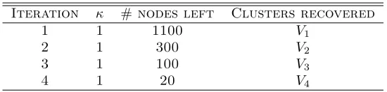
Iteration κ # nodes left Clusters recovered
1 1 1100 V1
2 1 300 V2
3 1 100 V3
4 1 20 V4
Table 1: Results for experiment 1: n= 1100, {|Va|}={800,200,80,20},p = 0.5,q = 0.2,
fixedρ= 1.
Iteration κ # nodes left Clusters recovered
1 1 1100 V1
2 1 300 V2
3 1 100 V3, V4
Table 2: Results for experiment 2: n= 1100, {|Va|}={800,200,50,50},p0 = 0.7,q0 = 0.1, fixedρ= 0.3.
cluster (compared to the input size at that iteration) is recovered exactly and removed. The experiment terminates in 3 iterations using 18 seconds. Results are shown in Table 2.
4.3 Experiment 3 (Partial Observation, Adaptive Sampling Rate)
We use the simplified version of Algorithm 4 described previously. We have n = 1100
with clusters V1, . . . , V4 of sizes 800,200,50,50. The graph is generated with p0 = 0.8 and
q0 = 0.2, and then adaptively sampled by the algorithm. The algorithm terminates in 3 iterations using 148 seconds. Table 3 shows the recovery result and the sampling rates used in each iteration. From the table we can see that the expected total number of observed entries used by the algorithm is
11002·0.125 + 3002·0.25 + 1002·0.55 = 179250,
which is 14.8% of all possible node pairs (the actual number of observations is very close to this expected value). In comparison, we perform another experiment using a non-adaptive sampling rate, for which we needρ= 97.5% in order to recover all the clusters in one shot. Therefore, our adaptive algorithm achieves a significant saving in the number of queries.
4.4 Experiment 3A
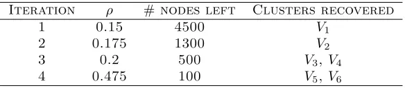
We repeat the above experiment with a larger instance: n= 4500 with clustersV1, . . . , V6
Iteration ρ # nodes left Clusters recovered
1 0.125 1100 V1
2 0.25 300 V2
3 0.55 100 V3,V4
Table 3: Results for experiment 3: n= 1100,{|Va|}={800,200,50,50},p0= 0.8, q0= 0.2.
Iteration ρ # nodes left Clusters recovered
1 0.15 4500 V1
2 0.175 1300 V2
3 0.2 500 V3,V4
4 0.475 100 V5,V6
Table 4: Results for experiment 3A: n = 4500, {|Va|} = {3200,800,200,200,50,50}, p0 = 0.8,q0= 0.2.
ρ = 35.0% only recovers the 4 largest clusters, and we are unable to recover all 6 clusters in one shot even withρ= 1 .
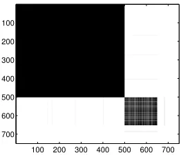
4.5 Experiment 4 (Mid-Size Clusters)
Our current theoretical results do not say anything about the mid-size clusters—those with sizes between`[ and`]. It is interesting to investigate the behavior of (CP) in the presence
of mid-size clusters. We generate an instance with n = 750 nodes partitioned into four
clusters of sizes {500,150,70,30}, edge probabilities p = 0.8, q = 0.2 and a sampling rate
ρ = 0.12. We then solve (CP) with a fixed κ = 1. The low-rank part K of the solution
is shown in Figure 2. The large cluster of size 500 is completely recovered in K, while the two small clusters of sizes 70 and 30 are entirely ignored. The medium cluster of size 150, however, exhibits a pattern we find difficult to characterize. This shows that the constant gap between`]and`[in our theorems is a real phenomenon and not an artifact of our proof
techniques. Nevertheless, the mid-size cluster appears clean, and might allow recovery using a simple combinatorial procedure. If this is true in general, it might not be necessary to search for a gap free of cluster sizes. In particular, perhaps for anyκ, (CP) identifies all large clusters above `] after a simple mid-size cleanup procedure, and ignores all other clusters. Understanding this phenomenon and its algorithmic implications is of much interest.
5. Proofs
We use the following notation and conventions throughout the proofs. With high probability
or w.h.p. means with probability at least 1−n−6. The expressions a∨b and a∧b mean
100 200 300 400 500 600 700 100
200
300 400 500 600 700
Figure 2: The solution to (CP) with mid-size clusters.
kMk1 is Pi,j|M(i, j)|, and kMk∞ is maxij|M(i, j)|. We shall use the standard inner
producthX, Yi:=Pn
i,j=1X(i, j)Y(i, j).
We will also study operators on the space of matrices, and denote them using a calli-graphic font, e.g.,P. The normkPkof an operator is defined as
kPk:= sup
M∈Rn×n:kMk F=1
kPMkF .
For a fixed real n×n matrixM, we define the matrix linear subspaceT(M) as follows:
T(M) :={Y M+M X :X, Y ∈Rn×n}.
In words, this subspace is the set of matrices spanned by matrices each row of which is in
the row space of M, and matrices each column of which is in the column space of M. We
letT(M)⊥ denote the orthogonal subspace toT(M) with respect toh·,·i, which is given by
T(M)⊥:={X∈Rn×n:hX, Yi= 0,∀Y ∈T(M)} .
It is a well known fact that the projection PT(X) onto T(X) w.r.t. h·,·i is given by
PT(X)M :=PC(X)M+PR(X)M − PC(X)PR(X)M ,
where PC(X) is projection (of each column of a matrix) onto the column space of X, and
PR(X) is projection onto the row space of X. The projection onto T(M)⊥ is PT(X)⊥M = M− PT(X)M .
Finally, we recall that s(M) is the support of M,Ps(M)X is the matrix obtained from
X by setting its entries outside s(M) to zero, and Ps(M)cX:=X− Ps(M)X. 5.1 Proof of Theorem 2
The proof builds on the analysis in Chen et al. (2012). We need some additional notation:
1. We let V[ ⊆ V denote the set of of elements i such that nhii ≤ `[. (We remind the
reader thatnhii=|Vhii|.)
2. We remind the reader that the projectionP] is defined as follows:
(P]M)(i, j) =
(
M(i, j), max{nhii, nhji} ≥`]
3. The projectionP[ is defined as follows:
(P[M)(i, j) =
(
M(i, j), max{nhii, nhji} ≤`[
0, otherwise.
In words,P[projects onto the set of matrices supported onV[×V[. Note that by the theorem assumption,P]+P[=Id(equivalently,P] projects onto the set of matrices
supported on (V ×V)\(V[×V[)).
4. We use UΣU> to denote the rank-k0 Singular Value Decomposition (SVD) of the symmetric matrix ˆK, wherek0 = rank( ˆK) and equals the number of clusters with size at least`].
5. Define the set
D:=
∆∈Rn×n|∆
ij ≤0,∀i∼j,(i, j)∈/ V[×V[; 0≤∆ij,∀i6∼j,(i, j)∈/V[×V[ ,
which strictly contains all feasible deviation from ˆK.
6. For simplicity we write T :=T( ˆK).
We will make use of the following facts:
1. Id=Ps( ˆB)+Ps( ˆB)c =Ps(A)+Ps(A)c.
2. P],P[,Ps( ˆB),Ps( ˆB)c,Ps(A),and Ps(A)c commute with each other.
5.1.1 Approximate Dual Certificate Condition
We begin by giving a deterministic sufficient condition for ( ˆK,Bˆ) to be the unique optimal solution to the program (CP).
Proposition 12 ( ˆK, B) is the unique optimal solution to (CP) if there exists a matrixˆ Q∈Rn×n and a number 0< <1 satisfying:
1. kQk<1;
2. kPT(Q)k∞≤
2min{c1, c2};
3. ∀∆∈D:
(a) DU U>+Q,Ps(A)Ps( ˆB)P]∆E= (1 +)c1
Ps(A)Ps( ˆB)P]∆ 1,
(b)
D
U U>+Q,Ps(A)cP
s( ˆB)P]∆ E
= (1 +)c2
Ps(A)cPs( ˆB)P]∆ 1;
4. ∀∆∈D:
(a)
D
U U>+Q,Ps(A)Ps( ˆB)cP]∆
E
≥ −(1−)c1
Ps(A)Ps( ˆB)cP]∆
1,
(b)
D
U U>+Q,Ps(A)cPs( ˆB)cP]∆
E
≥ −(1−)c2
5. Ps( ˆB)P[(U U>+Q) =c1P[Bˆ; 6.
Ps( ˆB)cP[(U U
>+Q)
∞≤c2.
Proof Consider any feasible solution ( ˆK + ∆,Bˆ −∆) to (CP); we know ∆ ∈ D due to the inequality constraints in (CP). We will show that this solution will have strictly higher objective value than ( ˆK,Bˆ) if ∆6= 0.
For this ∆, let G∆ be a matrix inT⊥∩Range(P[) satisfying kG∆k= 1 and hG∆,∆i= kPT⊥P[∆k∗; such a matrix always exists because RangeP[ ⊆ T⊥. Suppose kQk = b. Clearly, PT⊥Q+ (1−b)G∆ ∈ T⊥ and, due to Property 1 in the proposition, we have b < 1 and kPT⊥Q+ (1−b)G∆k ≤ kQk+ (1−b)kG∆k = b+ (1−b) = 1. Therefore, U U>+PT⊥Q+ (1−b)G∆is a subgradient of f(K) =kKk∗ atK= ˆK. On the other hand, define the matrix F∆ =−Ps( ˆB)csgn(∆). We have F∆ ∈s( ˆB)c and kF∆k∞ ≤1. Therefore, Ps(A)( ˆB +F∆) is a subgradient of g1(B) =
Ps(A)B
1 at B = ˆB, and Ps(A)c( ˆB +F∆)
is a subgradient of g2(B) =
Ps(A)cB
1 at B = ˆB. Using these three subgradients, the
difference in the objective value can be bounded as follows:
d(∆) , ˆ
K+ ∆
∗+c1
Ps(A)( ˆB−∆)
1+c2
Ps(A)c( ˆB−∆) 1 − ˆ K ∗−c1
Ps(A)
ˆ B 1 −c2
Ps(A)c
ˆ B 1
≥DU U>+PT⊥Q+ (1−b)G∆,∆
E
+c1 D
Ps(A)( ˆB+F∆),−∆ E
+c2 D
Ps(A)c( ˆB+F∆),−∆ E
=(1−b)kPT⊥P[∆k∗+
D
U U>+PT⊥Q,∆
E
+c1 D
Ps(A)B,ˆ −∆E+c2 D
Ps(A)cB,ˆ −∆ E
+c1
Ps(A)F∆,−∆
+c2
Ps(A)cF∆,−∆
=(1−b)kPT⊥P[∆k∗+
D
U U>+PT⊥Q,∆
E
+c1 D
P[Ps(A)B,ˆ −∆E+c2 D
P[Ps(A)cB,ˆ −∆ E
+c1 D
P]Ps(A)B,ˆ −∆ E
+c2 D
P]Ps(A)cB,ˆ −∆ E
+c1
Ps(A)F∆,−∆
+c2
Ps(A)cF∆,−∆
.
The last six terms of the last RHS satisfy:
1. c1 D
P[Ps(A)B,ˆ −∆
E
+c2 D
P[Ps(A)cB,ˆ −∆ E
=c1 D
P[B,ˆ −∆
E
, because P[Bˆ∈s(A).
2.
D
P]Ps(A)B,ˆ −∆
E ≥ −
P]Ps(A)Ps( ˆB)∆
1and D
P]Ps(A)cB,ˆ ∆ E
≥ −
P]Ps(A)cPs( ˆB)∆ 1,
because ˆB ∈s( ˆB) and
ˆ B ∞≤1.
3.
Ps(A)F∆,−∆
=
Ps(A)Ps( ˆB)c∆
1 and
Ps(A)cF∆,−∆=
Ps(A)cPs( ˆB)c∆
1, due to
the definition ofF.
It follows that
d(∆)≥(1−b)kPT⊥P[∆k∗+
D
U U>+PT⊥Q,∆
E
+c1 D
P[B,ˆ −∆E−c1
P]Ps(A)Ps( ˆB)∆ 1 −c2
P]Ps(A)cPs( ˆB)∆
1+c1
Ps(A)Psc( ˆB)∆
1+c2
Ps(A)cPsc∆
Consider the second term in the last RHS, which equals
D
U U>+PT⊥Q,∆
E
=DU U>+Q,P]∆
E
+DU U>+Q,P[∆E− hPTQ,∆i.
We bound these three terms separately. For the first term, we have
D
U U>+Q,P]∆
E
=DU U>+Q,Ps(A)Ps( ˆB)P]+Ps(A)cP
s( ˆB)P]+Ps(A)Ps( ˆB)cP]+Ps(A)cPscP]
∆E
≥(1 +)c1
Ps(A)Ps( ˆB)P]∆
1+ (1 +)c2
Ps(A)cPs( ˆB)P]∆
1−(1−)c1
Ps(A)Ps( ˆB)cP]∆ 1 −(1−)c2
Ps(A)cPs( ˆB)cP]∆
1. (Using Properties 3 and 4.)
For the second term, we have
D
U U>+Q,P[∆
E
=DPs( ˆB)P[(U U>+Q),∆E+DPs( ˆB)cP[(U U>+Q),∆
E
≥c1 D
P[B,ˆ ∆
E −c2
Ps( ˆB)cP[∆
1 (using Properties 5 and 6)
=c1 D
P[B,ˆ ∆
E −c2
Ps(A)cPs( ˆB)cP[∆
1. (Because Ps(A)
cPs( ˆB)cP[=Ps( ˆB)cP[.)
Finally, for the third term, Due to the block diagonal structure of the elements of T, we have PT =P]PT and therefore
h−PTQ,∆i=− hPTQ,P]∆i ≥ − kPTQk∞kP]∆k1≥ −
2min{c1, c2} kP]∆k1.
Combining the above three bounds with Eq. (11), we obtain
d(∆)
≥(1−b)kPT⊥P[∆k∗+c1
P]Ps(A)Ps( ˆB)∆
1+c2
P]Ps(A)cPs( ˆB)∆
1+c1
Ps(A)Ps( ˆB)cP]∆ 1
+c2
Ps(A)cPs( ˆB)cP]∆
1+c1
Ps(A)Ps( ˆB)cP[∆
1−
2min{c1, c2} kP]∆k1 =(1−b)kPT⊥P[∆k∗+c1
P]Ps(A)∆
1+c2
P]Ps(A)c∆
1−
2min{c1, c2} kP]∆k1
(note thatPs(A)Ps( ˆB)cP[∆=0)
≥(1−b)kP[∆k∗+
2min{c1, c2} kP]∆k1, which is strictly greater than zero for ∆6= 0.
5.1.2 Constructing Q
constructing Q. Suppose we take
:= p 100
t(1−t)max
(
κ√n `] ,
s
log4n `]
)
,
and use the weights c1 and c2 given in Theorem 2. We specifyP]Qand P[Q separately.
The matrix P]Q is given by P]Q=P]Q1+P]Q2+P]Q3, where for (i, j)∈/V[×V[,
P]Q1(i, j) =
−n1
hii, i∼j,(i, j)∈s( ˆB)
1
nhii ·
1−pij
pij , i∼j,(i, j)∈s( ˆB)
c
0, i6∼j
P]Q2(i, j) =
−(1 +)c2, i∼j,(i, j)∈s( ˆB)
(1 +)c21−pijpij, i∼j,(i, j)∈s( ˆB)c
0, i6∼j
P]Q3(i, j) =
(1 +)c1, i6∼j,(i, j)∈s( ˆB) −(1 +)c11−qijqij, i6∼j,(i, j)∈s( ˆB)c
0, i∼j.
Note that these matrices have zero-mean entries. (Recall that s( ˆB) = s(A−Kˆ) is a random set since the graphA is random.)
P[Q is given as follows. For (i, j)∈V[×V[,
P[Q(i, j) =
c1, i∼j,(i, j)∈s(A) −c2, i∼j,(i, j)∈s(A)c
c1, i6∼j,(i, j)∈s(A)
c2W(i, j), i6∼j,(i, j)∈s(A)c,
whereW is a symmetric matrix whose upper-triangle entries are independent and obey
W(i, j) =
(
+1, with probability 2t(1−t−qq),
−1, with remaining probability.
Note that we introduced additional randomness in W.
5.1.3 Validating Q
Under the choice of t in Theorem 2, we have 14p ≤ t ≤ p and 14(1−q) ≤ 1−t ≤ 1−q. Also under the assumption (1) in the theorem and since p−q ≤p(1−q),`] ≤n, we have
p(1−q)≥ b23κ2n
`2 ]
∨b3log4n
`] ≥
b3log4n
n . Using these inequalities, it is easy to check that <
1 2
provided that the constantb3is sufficiently large. We will make use of these facts frequently
in the proof.
Property 1:
Suppose the matrix Q∼ is obtained from Q by setting all Q(i, j) with i 6∼ j to zero,
and Q6∼ =Q−Q∼. Note that kQk ≤ kP]Q∼k+kP]Q6∼k+kP[Q∼k+kP[Q6∼k. Below we
show that with high probability, the first term is upper-bounded by 327 and the other threes terms are upper-bounded by 14, which establishes that kQk ≤ 3132 .
(a)P[Q∼is a block diagonal matrix support onV[×V[, where the size of each block is at
most`[. Note thatP[Q∼=E[P[Q∼] + (P[Q∼−E[P[Q∼]). HereE[P[Q∼] is a deterministic
matrix with all non-zero entries equal to 1001κ√
n p−t
√
t(1−t). We thus have kE[P[Q∼]k ≤`[
1 100κ√n
p−t
p
t(1−t) ≤ 1 32,
where the last inequality holds under the definition of `[ in Theorem 2. On the other
hand, the matrix P[Q∼ −E[P[Q∼] is a random matrix whose entries are independent,
bounded almost surely byB := max{c1, c2}and have zero mean with variance bounded by 1
1002κ2n·
p(1−p)
t(1−t).If `[≤n2/3, we apply part 1 of Lemma 17 to obtain
kP[Q∼−E[P[Q∼]k ≤10 max (
1 100κ√n
s
p(1−p)
t(1−t)`[logn,(c1∨c2) logn
) ≤max ( 1 10κ s
p(1−p)
t(1−t) logn
n1/3,
1 10κ√n
r
1−t
t ∨
r
t
1−t
!
logn
) ≤ 3
16,
where the last inequality follows fromt(1−t)≥ p(1−16q) & logn4n. If`[≥n2/3 ≥76, then the
variance of the entries is bounded by σ2 := 1002κ21nt(1−t)
p(1−p)∨t2log` 4n
[ ∨
(1−t)2log4n
`[
,
and σ& B√log`2n [
. Hence we can apply part 2 of Lemma 17 to get
kP[Q∼−E[P[Q∼]k ≤10σ p
`[≤ 3
16,w.h.p.,
where in the last inequality we use n≥`[ and t(1−t)≥ 1
16p(1−q) & log4n
n . We conclude
thatkP[Q∼k ≤ kE[P[Q∼]k+kP[Q∼−E[P[Q∼]k ≤ 321 +163 = 327 w.h.p.
(b)P[Q6∼ is a random matrix supported onV[×V[, whose entries are independent, zero
mean, bounded almost surely byB0 := max{c1, c2}, and have variance 10021κ2n·
t2+q−2tq (1−t)t .If `[≤n2/3, we apply part 1 of Lemma 17 to obtain
kP[Q6∼k ≤10 max (
1 100κ√n
s
t2+q−2tq
t(1−t) `[logn,(c1∨c2) logn
) ≤max ( 1 10κ s
t2+q−2tq
t(1−t)
logn n1/3,
1 10κ√n
r
1−t
t ∨
r
t
1−t
!
logn
) ≤ 1
4,
where the last inequality follows fromt(1−t)≥ p(1−16q) & logn4n. If`[ ≥n2/3 ≥76, one verifies
that the variance of the entries is bounded by (σ0)2 := 10021κ2n·
t2+q−2tq (1−t)t ∨
tlog4n (1−t)`[∨
(1−t) log4n t`[
and σ0& B0√log`2n [
.Hence we can apply part 2 of Lemma 17 to obtain
kP[Q6∼k ≤10σ0 p
`[≤
1
4,w.h.p.,
where in the last inequality we use n≥`[ and t(1−t)≥ 1
16p(1−q)& log4n
n .
(c) Note that P]Q∼ = P]Q1 +P]Q2. By construction these two matrices are both
block-diagonal, have independent zero-mean entries which are bounded almost surely by
B∼,1:= `1]p andB∼,2 := 2pc2 respectively, and and have variance bounded byσ∼21 := 1
p`2 ]
and
σ∼22 := 4(1−t)
p c22 respectively. One verifies that σ∼,i & B∼,ilog
2n √
n for i= 1,2. We can then
apply part 2 of Lemma 17 to obtain kP]Q∼k ≤10(σ∼,1+σ∼,2) √
n≤ 14 w.h.p.
(d) Note that P]Q6∼ = P]Q3 is a random matrix with independent zero-mean entries
which are bounded almost surely by B6∼ := 1−2c1q and have variance bounded by σ26∼ := 4t
1−qc
2
1. One verifies thatσ6∼≥
B6∼√log2n
n . We can then apply part 2 of Lemma 17 to obtain
kP]Q6∼k ≤4σ6∼ √
n≤ 1
4 w.h.p.
Property 2:
Due to the structure of T, we have
kPTQk∞=kPTP]Qk∞=
U U
>(P
]Q) + (P]Q)U U>+U U>(P]Q)U U>
∞ ≤3 U U >P ]Q ∞≤3
3 X m=1 U U >P
]Qm
∞.
Now observe that (U U>P]Qm)(i, j) = P
l∈Vhii
1
nhiiP]Qm(l, j) is the sum of independent zero-mean random variables with bounded magnitude and variance. Using the Bernstein inequality in Lemma 19, we obtain that for each (i, j) and with probability at least 1−n−8,
(U U
>P
]Q1)(i, j) ≤
10
nhii`] r
1−p
p ·
q
nhiilogn+
logn p ≤ 1 24κ s
log2n
n`] , w.h.p.,
where in the last inequality we use p & κ`22n ]
. For i ∈ V[, clearly (U U>P]Q1)(i, j) = 0.
By union bound we conclude that U U>P]Q1
∞ ≤ 241κ q
log2n
n`] w.h.p. We can bound
U U>P]Q2 ∞ and
U U>P]Q3
∞ in a similar fashion: for each (i, j) and with probability
at least 1−n−8:
(U U
>P
]Q2)(i, j) ≤10
(1 +)c2
nhii
r
1−p
p ·
q
nhiilogn+
logn p ≤ 15 100κ s t
(1−t)n ·
s
(1−p) logn
p`] + logn `]p ! ≤ 1 6κ s
where the last inequality follows from p(1−t)& log`]n, and
(U U
>P
]Q3)(i, j) ≤10
(1 +)c1
nhii
r q
1−q ·
q
nhiilogn+
logn
1−q
≤ 15
100κ
r
1−t
tn ·
s
qlogn
(1−q)`]
+ logn
`](1−q)
! ≤ 1
6κ
s
log2n n`]
,
where the last inequality follows from t(1−q) & log`]n. On the other hand, under the definition ofc1, c2 and , we have
c1≥
1 100κ
r
1−t tn ·100
s
log4n t(1−t)`] =
1
κt ·
s
log4n
n`] ≥
3
κ
s
log2n n`] ,
and similarly
c2≥
1 100κ
s
t
(1−t)n·100
s
log4n t(1−t)`]
≥ 3
κ
s
log2n n`]
.
It follows thatkPTQk∞≤3· 241 + 1 6 +
1 6
·3(c1∧c2)≤ 2(c1∧c2) w.h.p., proving Property 2).
Properties 3(a) and 3(b):
For 3(a), by construction of Qwe have
D
U U>+Q,Ps(A)Ps( ˆB)P]∆
E
=
D
Ps(A)Ps( ˆB)P]Q3,Ps(A)Ps( ˆB)P]∆
E
= (1 +)c1·
X
(i,j)∈s( ˆB)∩s(A)
P]∆(i, j)
= (1 +)c1
Ps(A)Ps( ˆB)P]∆
1,
where the last equality follows from ∆∈D. Similarly, since
Ps(A)cP
s( ˆB)P]Q1=Ps(A)cP
s( ˆB)P](−U U >),
we have
D
U U>+Q,Ps(A)cPs( ˆB)P]∆ E
=
D
Ps(A)cPs( ˆB)P]Q2,Ps(A)cPs( ˆB)P]∆ E
=−(1 +)c2·
X
(i,j)∈s( ˆB)∩s(A)c
P]∆(i, j)
= (1 +)c2
Ps(A)cPs( ˆB)P]∆
1,
where the last equality again follows from ∆∈D; this proves Property 3(b).
For 4(a), we have
D
U U>+Q,Ps(A)Ps( ˆB)cP]∆
E
=
D
Ps(A)Ps( ˆB)cP]
U U>+P]Q1+P]Q2
,Ps(A)Ps( ˆB)cP]∆
E
= X
(i,j)∈s( ˆB)c∩s(A)
1
nhii
+ 1
nhii
1−pij pij
+ (1 +)c2
1−pij pij
P]∆(i, j)
≥ −
1
p`] + (1 +)c2
1−p p
Ps(A)Ps( ˆB)cP]∆
1, (12)
where the last inequality follows from ∆∈D, pij ≥p and nhii ≥`],∀i ∈V]. Consider the
two terms in the parenthesis in (12). For the first term, we have
1
p`] =
100κ `]
r n
t(1−t) ·
s
t(1−t) 1002κ2p2n ≤
100κ `]
r n
t(1−t) · 1 100κ
r
1−t tn ≤c1.
For the second term in (12), we have the following:
p−t≥ p−q
4 ≥
1
4max
(
κpb3p(1−q)n
`] ,
s
b3p(1−q) log4n
`]
)
=
√
b3
4 ·p(1−t)·
p
t(1−q)
p
p(1−t) ·max
(
κ√n
`]pt(1−t),
s
log4n t(1−t)`]
)
≥8p(1−t)·100 max
(
κ√n `]
p
t(1−t),
s
log4n t(1−t)`]
)
= 8p(1−t).
A little algebra shows that this implies (1 +)
q
t
1−t
1−p
p ≤ (1−)
q 1−t
t , or equivalently
(1 +)c21−pp ≤(1−2)c1. Substituting back to (12), we conclude that D
U U>+Q,Ps(A)Ps( ˆB)cP]∆
E
≥ −(c1+ (1−2)c1)
Ps(A)Ps( ˆB)cP]∆
1,
proving Property 4(a). For 4(b), we have
D
U U>+Q,Ps(A)cP
s( ˆB)cP]∆
E
=DPs(A)cP
s( ˆB)cP]Q3,Ps(A)cP
s( ˆB)cP]∆
E
= X
(i,j)∈s(A)c∩s( ˆB)c
−(1 +) c1qij 1−qij
P]∆(i, j)
≥ −(1 +) c1q 1−q
Ps(A)cPs( ˆB)cP]∆
where the last inequality follows from qij ≤q. Consider the factor before the norm in (13).
Similarly as before, we have
t−q≥ p−q
4 ≥
1
4max
(
κpb3p(1−q)n
`]
,
s
b3p(1−q) log4n
`]
)
≥2t(1−q)·100 max
(
κ√n `]
p
t(1−t),
s
log4n t(1−t)`]
)
= 2t(1−q).
A little algebra shows that this implies (1 +)
q 1−t
t q
1−q ≤ (1−)
q
t
1−t, or equivalently
(1 +)c11−qq ≤(1−)c2. Substituting back to (13), we conclude that
D
U U>+Q,Ps(A)cP
s( ˆB)cP]∆
E
≥ −(1−)c2
Ps(A)cPs( ˆB)cP]∆
1,
proving Property 4(b).
Properties 5 and 6:
Note that P[U U> = 0 andPs( ˆB)P[ =Ps(A)P[. These two properties hold by construc-tion ofQ.
We note that Properties (3)-(6) hold deterministically.
Combining the above results and applying the union bound, we conclude that with probability at least 1−n−3, there exists a matrix Q (which is the one constructed and verified above) that satisfies the properties in Proposition 12, where the probability is with
respect to the randomness in the graph A and the matrix W. Since W is independent of
A, integrating out the randomness in W proves the theorem.
5.2 Proof of Theorem 5
To ease notation, throughout the proof, C denotes a general universal positive constant
that can take different values at different locations. We let Ω := s(B∗) denote the noise locations.
Fix κ ≥1 and t in the allowed range, let (K, B) be an optimal solution to (CP), and assumeK is a partial clustering induced byU1, . . . , Ur for some integer r, and also assume σmin(K) = mini∈[r]|Ui|satisfies (5). LetM =σmin(K). We need a few helpful facts. Note
that from the definition of t, c1, c2,
q+1
4(p−q)≤
c2
c1+c2
=t≤p− 1
4(p−q) . (14)
We say that a pair of sets Y ⊆V, Z ⊆V is cluster separated if there is no pair (y, z)∈
Y ×Z satisfying y∼z.
Assumption 13 For all pairs of cluster-separated sets Y, Z of size at least m := C(p−logq)n2
each,
|dˆY,Z−q|<
1
4(p−q) , (15)
This is proven by a Hoeffding tail bound and a union bound to hold with probability at least 1−n−4. To see why, fix the sizes mY, mZ of |Y|,|Z|, assumemY ≤mZ w.l.o.g. For each such choice, there are at most exp{C(mY+mZ) logn} ≤exp{2CmZlogn}possibilities
for the choice of sets Y, Z. For each such choice, the probability that (15) does not hold is
exp{−CmYmZ(p−q)2} (16)
using Hoeffding inequality. Hence, as long asmY ≥mas defined above, using union bound
(over all possibilities of mY, mZ and ofY, Z) we obtain (15) uniformly. If we also assume that
M ≥3m , (17)
the implication of Assumption 13 is that it cannot be the case that some Ui contains a
subset Ui0 of size in the range [m,|Ui| −m] such thatUi0 =Vg∩Ui for someg. Otherwise,
if such a set existed, then we would find a strictly better solution to (CP), call it (K0, B0), which is defined so that K0 is obtained fromK by splitting the block corresponding to Ui
into two blocks, one corresponding toUi0and the other toUi\Ui0. The difference ∆ between
the cost of (K, B) and (K0, B0) is (renamingY :=Ui0 and Z :=U\Ui0)
∆ =c1|(Y ×Z)∩Ω| −c2|(Y ×Z)∩Ωc|= (c1+c2) ˆdY,Z|Y| |Z| −c2|Y| |Z|.
But the sign of ∆ is exactly the sign of ˆdY,Z −c1c+2c2 which is strictly negative by (15) and
(14). (We also used the fact that the trace norm part of the utility function is equal for both solutions: kK0k∗ =kKk∗).
The conclusion is that for each i, the sets (Ui∩V1), . . . ,(Ui∩Vk) must all be of size at
most m, except maybe for at most one set of size at least |Ui| −m. But note that by the theorem’s assumption,
M > km= (kClogn)/(p−q)2 , (18)
so we conclude that not all the sets (Ui∩V1), . . . ,(Ui∩Vk) can be of size at mostm. Hence
exactly one of these sets must have size at least|Ui| −m. From this we conclude that there
is a functionφ: [r]7→[k] such that for alli∈[r],
|Ui∩Vφ(i)| ≥ |Ui| −m .
We now claim that this function is an injection. We will need the following assumption:
Assumption 14 For any 4 pairwise disjoint subsets(Y, Y0, Z, Z0) such that (Y ∪Y0)⊆Vi for some i,(Z∪Z0)⊆[n]\Vi, max{|Z|,|Z0|} ≤m, min{|Y|,|Y0|} ≥M−m:
|Y| · |Y0|dˆY,Y0− |Y| · |Z|dˆY,Z − |Y0| · |Z0|dˆY0,Z0 > c2
c1+c2
(|Y| · |Y0| − |Y| · |Z| − |Y0| · |Z0|) (19)
The assumption holds with probability at least 1−n−4 by using Hoeffding inequality,
union bounding over all possible sets Y, Y0, Z, Z0 as above. Indeed, notice that for fixed
mY, mY0, mZ, mZ0 (with, say, mY ≥mY0), and for each tuple Y, Y0, Z, Z0 such that|Y|= mY,|Y0|=mY0,|Z|=mZ,|Z0|=mZ0, the probability that (19) is violated is at most