An Efﬁcient Boosting Algorithm for Combining Preferences

(1)

An Efficient Boosting Algorithm for Combining Preferences

Yoav Freund

Center for Computational Learning Systems Columbia University

500 West 120th St.

New York, NY 10027 [email protected]

Raj Iyer

Living Wisdom School 456 College Avenue

Palo Alto, CA 94306 [email protected]

Robert E. Schapire

Department of Computer Science Princeton University

35 Olden Street

Princeton, NJ 08544 [email protected]

Yoram Singer

School of Computer Science & Engineering Hebrew University

Jerusalem 91904, Israel [email protected]

Editor: Thomas G. Dietterich

Abstract

We study the problem of learning to accurately rank a set of objects by combining a given collec-tion of ranking or preference funccollec-tions. This problem of combining preferences arises in several applications, such as that of combining the results of different search engines, or the “collaborative-filtering” problem of ranking movies for a user based on the movie rankings provided by other users. In this work, we begin by presenting a formal framework for this general problem. We then describe and analyze an efficient algorithm called RankBoost for combining preferences based on the boosting approach to machine learning. We give theoretical results describing the algorithm’s behavior both on the training data, and on new test data not seen during training. We also describe an efficient implementation of the algorithm for a particular restricted but common case. We next discuss two experiments we carried out to assess the performance of RankBoost. In the first exper-iment, we used the algorithm to combine different web search strategies, each of which is a query expansion for a given domain. The second experiment is a collaborative-filtering task for making movie recommendations.

1. Introduction

(2)

provided by other viewers and uses this information to return to Alice a list of recommended movies. To do that, the recommendation system looks for viewers whose preferences are similar to Alice’s and combines their preferences to make its recommendations.

In this paper, we introduce and study an efficient learning algorithm called RankBoost for com-bining multiple rankings or preferences (we use these terms interchangeably). This algorithm is based on Freund and Schapire’s (1997) AdaBoost algorithm and its recent successor developed by Schapire and Singer (1999). Similar to other boosting algorithms, RankBoost works by combining many “weak” rankings of the given instances. Each of these may be only weakly correlated with the target ranking that we are attempting to approximate. We show how to combine such weak rankings into a single highly accurate ranking.

We study the ranking problem in a general learning framework described in detail in Section 2. Roughly speaking, in this framework, the goal of the learning algorithm is simply to produce a single linear ordering of the given set of objects by combining a set of given linear orderings called the

ranking features. As a form of feedback, the learning algorithm is also provided with information

about which pairs of objects should be ranked above or below one another. The learning algorithm then attempts to find a combined ranking that misorders as few pairs as possible, relative to the given feedback.

In Section 3, we describe RankBoost in detail and we prove a theorem about its effectiveness on the training set. We also describe an efficient implementation for “bipartite feedback,” a special case that occurs naturally in many domains. We analyze the complexity of all of the algorithms studied.

In Section 4, we describe an efficient procedure for finding the weak rankings that will be combined by RankBoost using the ranking features. For instance, for the movie task, this procedure translates into using very simple weak rankings that partition all movies into only two equivalence sets, those that are more preferred and those that are less preferred. Specifically, we use another viewer’s ranked list of movies partitioned according to whether or not he prefers them to a particular movie that appears on his list. Such partitions of the data have the advantage that they only depend on the relative ordering defined by the given rankings rather than absolute ratings. In other words, even if the ranking of movies is expressed by assigning each movie a numeric score, we ignore the numeric values of these scores and concentrate only on their relative order. This distinction becomes very important when we combine the rankings of many viewers who often use completely different ranges of scores to express identical preferences. Situations where we need to combine the rankings of different models also arise in meta-searching problems (Etzioni et al., 1996) and in information-retrieval problems (Salton, 1989, Salton and McGill, 1983).

In Section 5, for a particular probabilistic setting, we study the generalization performance of RankBoost, that is, how we expect it to perform on test data not seen during training. This analysis is based on a uniform-convergence theorem that we prove relating the performance on the training set to the expected performance on a separate test set.

(3)

The second problem is the movie-recommendation problem described above. For this problem, there exists a large publicly available dataset that contains ratings of movies by many different people. We compared RankBoost to nearest-neighbor and regression algorithms that have been previously studied for this application using several evaluation measures. RankBoost was the clear winner in these experiments.

In addition to the experiments that we report, Collins (2000) and Walker, Rambow, and Rogati (2001) describe recent experiments using the RankBoost algorithm for natural-language processing tasks. Also, in a recent paper (Iyer et al., 2000), two versions of RankBoost were compared to traditional information retrieval approaches.

Despite the wide range of applications that use and combine rankings, this problem has received relatively little attention in the machine-learning community. The few methods that have been devised for combining rankings tend to be based either on nearest-neighbor methods (Resnick et al., 1995, Shardanand and Maes, 1995) or gradient-descent techniques (Bartell et al., 1994, Caruana et al., 1996). In the latter case, the rankings are viewed as real-valued scores and the problem of combining different rankings reduces to numerical search for a set of parameters that will minimize the disparity between the combined scores and the feedback of a user.

While the above (and other) approaches might work well in practice, they still do not guarantee that the combined system will match the user’s preference when we view the scores as a means to express preferences. Cohen, Schapire and Singer (1999) proposed a framework for manipulating and combining multiple rankings in order to directly minimize the number of disagreements. In their framework, the rankings are used to construct preference graphs and the problem is reduced to a combinatorial optimization problem which turns out to be NP-complete; hence, an approximation is used to combine the different rankings. They also describe an efficient on-line algorithm for a related problem.

The algorithm we present in this paper uses a similar framework to that of Cohen, Schapire and Singer, but avoids the intractability problems. Furthermore, as opposed to their on-line algorithm, RankBoost is more appropriate for batch settings where there is enough time to find a good com-bination. Thus, the two approaches complement each other. Together, these algorithms constitute a viable approach to the problem of combining multiple rankings that, as our experiments indicate, works very well in practice.

2. A Formal Framework for the Ranking Problem

In this section, we describe our formal model for studying ranking.

Let

X

be a set called the domain or instance space. Elements of

X

are called instances. These

are the objects that we are interested in ranking. For example, in the movie-ranking task, each movie is an instance.

Our goal is to combine a given set of preferences or rankings of the instance space. We use the term ranking feature to denote these given rankings of the instances. A ranking feature is nothing more than an ordering of the instances from most preferred to least preferred. To make the model flexible, we allow ties in this ordering, and we do not require that all of the instances be ordered by every ranking feature.

We assume that a learning algorithm in our model is given n ranking features denoted f1, . . . ,fn.

Since each ranking feature fidefines a linear ordering of the instances, we can equivalently think of

(4)

can represent any ranking feature as a real-valued function where fi(x1)>fi(x0)means that instance x1 is preferred to x0by fi. The actual numerical values of fi are immaterial; only the ordering that

they define is of interest. Note that this representation also permits ties (since fi can assign equal

values to two instances).

As noted above, it is often convenient to permit a ranking feature fito “abstain” on a particular

instance. To represent such an abstention on a particular instance x, we simply assign fi(x) the

special symbol _⊥which is incomparable to all real numbers. Thus, fi(x) =⊥indicates that no

ranking is given to x by fi. Formally, then, each ranking feature fiis a function of the form fi:

X

→

R, where the setRconsists of all real numbers, plus the additional element_⊥.

Ranking features are intended to provide a base level of information about the ranking task. Said differently, the learner’s job will be to learn a ranking expressible in terms of the primitive ranking features, similar to ordinary features in more conventional learning settings. (However, we choose to call them “ranking features” rather than simply “features” to stress that they have a particular form and function.)

For example, in one formulation of the movie task, each ranking feature corresponds to a single viewer’s past ratings of movies, so there are as many ranking features as there are past users of the recommendation service. Movies which were rated by that viewer are assigned the viewer’s numerical rating of the movie; movies which were not rated at all by that viewer are assigned the special symbol _⊥to indicate that the movie was not ranked. Thus, fi(x) is movie-viewer i’s

numerical rating of movie x, or_⊥if no rating was provided.

The goal of learning is to combine all of the ranking functions into a single ranking of the instances called the final or combined ranking. The final ranking should have the same form as that of the ranking features; that is, it should give a linear ordering of the instances (with ties allowed). However, unlike ranking features, we do not permit the final ranking to abstain on any instances, since we want to be able to rank all instances, even those not seen during training. Thus, formally

the final ranking can be represented by a function H :

X

_→Rwith a similar interpretation to that

of the ranking features, i.e., x1 is ranked higher than x0 by H if H(x1)>H(x0). Note the explicit

omission of_⊥from the range of H, thus prohibiting abstentions. For example, for the movie task,

this corresponds to a complete ordering of all movies (with ties allowed), where the most highly recommended movies at the top of the ordering have the highest scores.

Finally, we need to assume that the learner has some feedback information describing the desired form of the final ranking. Note that this information is not encoded by the ranking features, which are merely the primitive elements with which the learner constructs its final ranking. In traditional classification learning, this feedback would take the form of labels on the examples which indicate the correct classification. Here our goal is instead to come up with a good ranking of the instances, so we need some feedback describing, by example, what it means for a ranking to be “good.”

(5)

However, in other domains, this form and representation of feedback information may be overly restrictive. For instance, in some cases, two instances may be entirely unrelated and we may not care about how they compare. For example, suppose we are trying to rate individual pieces of fruit. We might only have information about how individual apples compare with other apples, and how oranges compare with oranges; we might not have information comparing apples and oranges. A more realistic example is given by the meta-search task described in Section 2.1.

Another difficulty with restricting the feedback to be a linear ordering is that we may consider it very important (because of the strength of available evidence) to rank instance x1above x0, but

only slightly important that instance x2 be ranked above x3. Such variations in the importance of

how instances are ranking against one another cannot be easily represented using a simple linear ordering of the instances.

To allow for the encoding of such general feedback information, we instead assume that the learner is provided with information about the relative ranking of individual pairs of instances. That is, for every pair of instances x0,x1, the learner is informed as to whether x1should be ranked above

or below x0, and also how important or how strong is the evidence that this ranking should exist. All

of this information can be conveniently represented by a single functionΦ. The domain ofΦis all pairs of instances. For any pair of instances x0,x1,Φ(x0,x1)is a real number whose sign indicates

whether or not x1 should be ranked above x0, and whose magnitude represents the importance of

this ranking.

Formally, then, we assume the feedback function has the formΦ:

X

_×

X

_→R. Here,Φ(x0,x1)>

0 means that x1should be ranked above x0whileΦ(x0,x1)<0 means the opposite; a value of zero

indicates no preference between x0and x1. As noted above, the larger the magnitude|Φ(x0,x1)|, the

more important it is to rank x1above or below x0. Consistent with this interpretation, we assume

thatΦ(x,x) =0 for all x_∈

X

, and thatΦis anti-symmetric in the sense thatΦ(x0,x1) =−Φ(x1,x0)

for all x0,x1∈

X

. Note, however, that we do not assume transitivity of the feedback function.1

For example, for the movie task, we can defineΦ(x0,x1)to be+1 if movie x1was preferred to

movie x0by Alice,−1 if the opposite was the case, and 0 if either of the movies was not seen or if

they were equally rated.

As suggested above, a learning algorithm typically attempts to find a final ranking that is similar to the given feedback function. There are perhaps many possible ways of measuring such simi-larity. In this paper, we focus on minimizing the (weighted) number of pairs of instances which are misordered by the final ranking relative to the feedback function. To formalize this goal, let

D(x0,x1) =c·max{0,Φ(x0,x1)}so that all negative entries ofΦ(which carry no additional

infor-mation) are set to zero. Here, c is a positive constant chosen so that

∑

x0,x1

D(x0,x1) =1.

(When a specific range is not specified on a sum, we always assume summation over all of

X

.) Let

us define a pair x0,x1to be crucial ifΦ(x0,x1)>0 so that the pair receives non-zero weight under D.

The learning algorithms that we study attempt to find a final ranking H with a small weighted number of crucial-pair misorderings, a quantity called the ranking loss and denoted rlossD(H).

1. In fact, we do not even use the property thatΦis anti-symmetric, so this condition also could be dropped. For instance, we might instead formalizeΦto be a nonnegative function in which a positive value forΦ(x0,x1)indicates that x1

should be ranked higher than x0, but there is no prohibition against bothΦ(x0,x1)andΦ(x1,x0)being positive. This

might be helpful when we have contradictory evidence regarding the “true” ranking of x0and x1, and is analogous in

(6)

Formally, the ranking loss is defined to be

∑

x0,x1

D(x0,x1) [[H(x1)≤H(x0)]] =Pr(x0,x1)∼D[H(x1)≤H(x0)]. (1)

Here and throughout this paper, we use the notation[[π]]which is defined to be 1 if predicateπholds and 0 otherwise.

There are many other ways of measuring the quality of a final ranking. Some of these alternative measures are described and used in Section 6.

Of course, the real purpose of learning is to produce a ranking that performs well even on instances not observed in training. For instance, for the movie task, we would like to find a ranking of all movies that accurately predicts which ones a movie-viewer will like more or less than others; obviously, this ranking is only of value if it includes movies that the viewer has not already seen. As in other learning settings, how well the learning system performs on unseen data depends on many factors, such as the number of instances covered in training and the representational complexity of the ranking produced by the learner. Some of these issues are addressed in Section 5.

into a single functionΦsimply by adding them: Φ=∑_jΦj. (If some have greater importance than

others, then a weighted sum can be used.)

2.1 Example: Meta-search

To illustrate this framework, we now describe the meta-search problem and how it fits into the general framework. Experiments with this problem are described in Section 6.1.

For this task, we used the data of Cohen, Schapire and Singer (1999). Their goal was to simulate the problem of building a domain-specific search engine. As test cases, they picked two fairly narrow classes of queries—retrieving the homepages of machine-learning researchers (ML), and retrieving the homepages of universities (UNIV). They chose these test cases partly because the feedback was readily available from the web. They obtained a list of machine-learning researchers, identified by name and affiliated institution, together with their homepages,2 and a similar list for universities, identified by name and (sometimes) geographical location from Yahoo! We refer to each entry on these lists (i.e., a name-affiliation pair or a name-location pair) as a base query. The goal is to learn a meta-search strategy that, given a base query, will generate a ranking of URLs that includes the correct homepage at or close to the top.

(7)

Cohen, Schapire and Singer also constructed a series of special-purpose search templates for each domain. Each template specifies a query expansion method for converting a base query into a likely seeming AltaVista query which we call the expanded query. For example, one of the

templates has the form+"NAME" +machine +learningwhich means that AltaVista should search

for all the words in the person’s name plus the words ‘machine’ and ‘learning’. When applied to the base query “Joe Researcher from Shannon Laboratory in Florham Park” this template expands

to the expanded query+"Joe Researcher" +machine +learning.

A total of 16 search templates were used for the ML domain and 22 for the UNIV domain.3

Each search template was used to retrieve the top thirty ranked documents. If none of these lists contained the correct homepage, then the base query was discarded from the experiment. In the ML domain, there were 210 base queries for which at least one search template returned the correct homepage; for the UNIV domain, there were 290 such base queries.

We mapped the meta-search problem into our framework as follows. Formally, the instances now are pairs of the form(q,u)where q is a base query and u is one of the URLs returned by one of the search templates for this query. Each ranking feature fiis constructed from a corresponding

search template i by assigning the jth URL u on its list (for base query q) a rank of ₋j; that is, fi((q,u)) =−j. If u is not ranked for this base query, then we set fi((q,u)) =⊥. We also construct

a separate feedback function Φq for each base query q that ranks the correct homepage URL u∗

above all others. That is, Φq((q,u),(q,u∗)) = +1 and Φq((q,u∗),(q,u)) =−1 for all u6=u∗. All

other entries of Φq are set to zero. All the feedback functions Φq were then combined into one

feedback functionΦby summing as described earlier: Φ=∑qΦq.

The output of a learning algorithm is some final ranking H. In the meta-search example H is a weighted combination of the different search templates fi. To apply H, given a test base query q, we

first form all of the expanded queries from search templates and send these to the search engine to obtain lists of URLs. We then evaluate H on each pair(q,u), where u is a returned URL, to obtain a predicted ranking of all of the URLs.

3. A Boosting Algorithm for the Ranking Task

In this section, we describe an approach to the ranking problem based on a machine learning method called boosting, in particular, Freund and Schapire’s (1997) AdaBoost algorithm and its successor developed by Schapire and Singer (1999). Boosting is a method of producing highly accurate prediction rules by combining many “weak” rules which may be only moderately accurate. In

instances indicates a great importance that the weak learner order that pair correctly.

(8)

Algorithm RankBoost

Given: initial distribution D overX_×X. Initialize: D1=D.

For t=1, . . . ,T :

• Train weak learner using distribution Dt.

• Get weak ranking ht:X→R.

• Chooseαt ∈R.

• Update: Dt+1(x0,x1) =

Dt(x0,x1)exp(αt(ht(x0)−ht(x1)))

Zt

where Zt is a normalization factor (chosen so that Dt+1will be a distribution).

Output the final ranking: H(x) =

T

∑

t=1

αtht(x)

Figure 1: The RankBoost algorithm.

Weak rankings have the form ht :

X

→R. We think of these as providing ranking information

in the same manner as ranking features and the final ranking. The weak learner we used in our experiments is based on the given ranking features; details are given in Section 4.

The boosting algorithm uses the weak rankings to update the distribution as shown in Figure 1. Suppose that x0,x1is a crucial pair so that we want x1to be ranked higher than x0(in all other cases, Dt will be zero). Assuming for the moment that the parameter αt >0 (as it usually will be), this

rule decreases the weight Dt(x0,x1)if ht gives a correct ranking (ht(x1)>ht(x0)) and increases the

weight otherwise. Thus, Dt will tend to concentrate on the pairs whose relative ranking is hardest

to determine. The actual setting ofαt will be discussed shortly.

The final ranking H is a weighted sum of the weak rankings. In the following theorem we prove

a bound on the ranking loss of H. This theorem also provides guidance in choosingαt and in

de-signing the weak learner as we discuss below. on the training data. As in standard classification problems, the loss on a separate test set can also be theoretically bounded given appropriate as-sumptions using uniform-convergence theory (Bartlett, 1998, Haussler, 1992, Schapire et al., 1998, Vapnik, 1982). In Section 5 we will derive one such bound on the ranking generalization error of

H and explain why the classification generalization error bounds do not trivially carry over to the

ranking setting.

Theorem 1 Assuming the notation of Figure 1, the ranking loss of H is

rlossD(H)≤ T

∏

t=1 Zt .

Proof: Unraveling the update rule, we have that

x0,x1

Dt(x0,x1)exp(αt(ht(x0)−ht(x1))).

Formally, RankBoost uses the weak learner as a black box and has no control over how it chooses its weak rankings. In practice, however, we are often faced with the task of implementing the weak learner, in which case we can design it to minimize Zt.

There are various methods for achieving this end. Here we sketch three. Let us fix t and drop all t subscripts when clear from context. (In particular, for the time being, D will denote Dt rather

than an initial distribution.)

First method. First and most generally, for any given weak ranking h, it can be shown that Z,

viewed as a function ofα, has a unique minimum which can be found numerically via a simple

binary search (except in trivial degenerate cases). For details, see Section 6.2 of Schapire and Singer (1999).

Second method. The second method of minimizing Z is applicable in the special case that h has range{0,1}. In this case, we can minimize Z analytically as follows: For b∈ {−1,0,+1}, let

Wb=

∑

x0,x1

D(x0,x1) [[h(x0)−h(x1) =b]].

Also, abbreviate W+1by W+and W−1by W−. Then Z=W−e−α+W0+W+eα.Using simple calculus, it can be verified that Z is minimized by setting

α=1

2ln

W₋ W+

(2)

which yields

Z=W0+2

p

W₋W+. (3)

Thus, if we are using weak rankings with range restricted to_{0,1_}, we should attempt to find h that

tends to minimize Equation (3) and we should then setαas in Equation (2).

Third method. For weak rankings with range[0,1], we can use a third method of settingαbased on an approximation of Z. Specifically, by the convexity of eαxas a function of x, it can be verified that

eαx_≤

1+x

2

eα+

1₋x

2

(10)

for all realαand x_∈[₋1,+1]. Thus, we can approximate Z by

Z _≤

∑

x0,x1

D(x0,x1)

1+h(x0)−h(x1)

2

eα+

1₋h(x0) +h(x1)

2

e−α

=

1₋r

2

eα+

1+r

2

e−α (4)

where

r=

∑

x0,x1

D(x0,x1)(h(x1)−h(x0)). (5)

The right hand side of Equation (4) is minimized when

α=1

2ln

1+r

1₋r

(6)

which, plugging into Equation (4), yields Z_≤√1₋r2_{. Thus, to approximately minimize Z using}

weak rankings with range[0,1], we can attempt to maximize_|r_|as defined in Equation (5) and then setαas in Equation (6). This is the method used in our experiments.

We now consider the case when any of these three methods for settingαassign a weak ranking

h a weightα<0. For example, according to Equation (2),αis negative if W+, the weight of mis-ordered pairs, is greater than W₋, the weight of correctly ordered pairs. Similarly for Equation (6),

α<0 if r<0 (note that r=W₋₋W+). Intuitively, this means that h is negatively correlated with the feedback; the reverse of its predicted order will better approximate the feedback. RankBoost allows such weak rankings and its update rule reflects this intuition: the weights of the pairs that h correctly orders are increased, and the weights of the incorrect pairs are decreased.

3.3 An Efficient Implementation for Bipartite Feedback

In this section, we describe a more efficient implementation of RankBoost for feedback of a special form. We say that the feedback function is bipartite if there exist disjoint subsets X0 and X1 of

X

such that Φ ranks all instances in X1 above all instances in X0 and says nothing about any other

pairs. That is, formally, for all x0∈X0and all x1∈X1we have thatΦ(x0,x1) = +1,Φ(x1,x0) =−1

andΦis zero on all other pairs.

Such feedback arises naturally, for instance, in document rank-retrieval tasks common in the field of information retrieval. Here, a set of documents may have been judged to be relevant or irrelevant. A feedback function that encodes these preferences will be bipartite. The goal of an algorithm for this task is to discover the relevant documents and present them to a user. Rather than output a classification of documents as relevant or irrelevant, the goal here is to output a ranked list of all documents that tends to place all relevant documents near the top of the list. One reason a ranking is preferred over a hard classification is that a ranking expresses the algorithm’s confidence in its predictions. Another reason is that typically users of ranked-retrieval systems do not have the patience to examine every document that was predicted as relevant, especially if there is large number of such documents. A ranking allows the system to guide the user’s decisions about which documents to read.

(11)

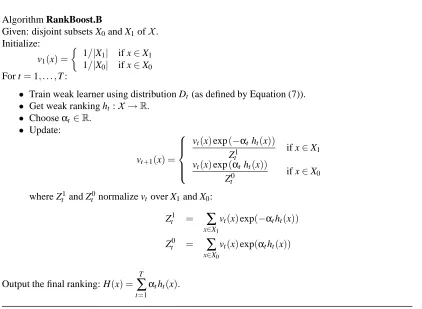
Algorithm RankBoost.B

Given: disjoint subsets X0and X1ofX.

Initialize:

v1(x) =

1/|X1| if x∈X1

1/|X0| if x∈X0

For t=1, . . . ,T :

• Train weak learner using distribution Dt(as defined by Equation (7)).

• Get weak ranking ht:X→R.

• Chooseαt ∈R.

• Update:

vt+1(x) =    

  

vt(x)exp(−αtht(x))

Z_t1 if x∈X1 vt(x)exp(αtht(x))

Z_t0 if x∈X0 where Z_t1and Z_t0normalize vt over X1and X0:

Z_t1 =

∑

x_∈X1

vt(x)exp(−αtht(x))

Z_t0 =

∑

x∈X0

vt(x)exp(αtht(x))

Output the final ranking: H(x) =

T

∑

t=1

αtht(x).

Figure 2: A more efficient version of RankBoost for bipartite feedback.

instance, this is the case for the meta-search problem described in Sections 2.1 and 6.1. However, for the sake of simplicity, we omit a full description of this straightforward extension and instead restrict our attention to the simpler case.

If RankBoost is implemented naively as in Section 3.2, then the space and time-per-round re-quirements will be O(_|X0| |X1|). In this section, we show how this can be improved to O(_|X0|+_|X1|). Note that, in this section,

X

_Φ=X0∪X1.

The main idea is to maintain a set of weights vt over

X

Φ(rather than the two-argument

distribu-tion Dt), and to maintain the condition that, on each round,

Dt(x0,x1) =vt(x0)vt(x1) (7)

for all crucial pairs x0,x1(recall that Dt is zero for all other pairs).

The pseudocode for this implementation is shown in Figure 2. Equation (7) can be proved by induction on t. It clearly holds initially. Using our inductive hypothesis, it is straightforward to expand the computation of Zt =Zt0·Zt1in Figure 2 to see that it is equivalent to the computation of

Zt in Figure 1. To show that Equation (7) holds on round t+1, we have, for crucial pair x0,x1: Dt+1(x0,x1) =

Dt(x0,x1)exp(αt(ht(x0)−ht(x1))) Zt

= vt(x0)exp(αtht(x0))

Z_t0 ·

vt(x1)exp(−αtht(x1)) Z_t1

(12)

Finally, note that all space requirements and all per-round computations are O(_|X0|+|X1|), with

the possible exception of the call to the weak learner. Fortunately, if we want the weak learner to maximize_|r_|as in Equation (5), then we also only need to pass|X_Φ_|weights to the weak learner, all of which can be computed in time linear in|X_Φ_|. Omitting t subscripts, and defining

s(x) =

+1 if x∈X1 −1 if x_∈X0

,

we can rewrite r as

r =

∑

x0,x1

D(x0,x1)(h(x1)−h(x0))

=

∑

x0∈X0

∑

x1∈X1

v(x0)v(x1) (h(x1)s(x1) +h(x0)s(x0))

=

∑

x0∈X0

v(x0)

∑

x1∈X1

v(x1)

!

s(x0)h(x0) +

∑

x1∈X1

v(x1)

∑

x0∈X0

v(x0)

!

s(x1)h(x1)

=

∑

x

d(x)s(x)h(x) (8)

where

d(x) =v(x)

∑

x0_:s₍_x₎₆₌_s₍_x0₎

v(x0).

All of the weights d(x)can be computed in linear time by first computing the sums that appear in this equation for the two possible cases that x is in X0or X1. Thus, we only need to pass|X0|+|X1|

weights to the weak learner in this case rather than the full distribution Dt of size|X0| |X1|. 4. Finding Weak Rankings

As described in Section 3, our algorithm RankBoost requires access to a weak learner to produce weak rankings. In this section, we describe an efficient implementation of a weak learner for rank-ing.

Perhaps the simplest and most obvious weak learner would find a weak ranking h that is equal to one of the ranking features fi, except on unranked instances. That is,

h(x) =

fi(x) if fi(x)∈R

qdef if fi(x) =⊥

for some qdef∈R.

(13)

For these reasons, we focus in this section and in our experiments on_{0,1_}-valued weak rank-ings that use the ordering information provided by the ranking features, but ignore specific scoring information. In particular, we will use weak rankings h of the form

h(x) = 





1 if fi(x)>θ

0 if fi(x)≤θ

qdef if fi(x) =⊥

(9)

where θ_∈R and qdef∈ {0,1}. That is, a weak ranking is derived from a ranking feature fi by

comparing the score of fi on a given instance to a threshold θ. To instances left unranked by fi,

the weak ranking assigns the default score qdef. For the remainder of this section, we show how to

choose the “best” feature, threshold, and default score.

Since our weak rankings are _{0,1_}-valued, we can use either the second or third methods de-scribed in Section 3.2 to guide us in our search for a weak ranking. We chose the third method because we can implement it more efficiently than the second. According to the second method, the weak learner should seek a weak ranking that minimizes Equation (3). For a given candidate weak ranking, we can directly compute the quantities W0,W₋, and W+, as defined in Section 3.2, in O(_|Φ_|)time. Moreover, for each of the n ranking features, there are at most|X_Φ_|+1 thresholds to consider (as defined by the range of fi on

X

Φ) and two possible default scores (0 and 1). Thus

a straightforward implementation of the second method requires O(n_|Φ_||

X

Φ|) time to generate a weak ranking.

The third method of Section 3.2 requires maximizing |r| as given by Equation (5) and has the

disadvantage that it is based on an approximation of Z. However, although a straightforward im-plementation also requires O(n_|Φ_||

X

_Φ_|)time, we will show how to implement it in O(n_|

X

_Φ_|+_|Φ_|) time. (In the case of bipartite feedback, if the boosting algorithm of Section 3.3 is used, only

O(n_|

X

Φ|)time is needed.) This is a significant improvement from the point of view of our experi-ments in which_|Φ_|was large.

We now describe a time and space efficient algorithm for maximizing_|r_|. Let us fix t and drop it from all subscripts to simplify the notation. We begin by rewriting r for a given D and h as follows:

r =

∑

x0,x1

D(x0,x1) (h(x1)−h(x0))

=

∑

x0,x1

D(x0,x1)h(x1)−

∑

x0,x1

D(x0,x1)h(x0)

=

∑

x

h(x)

∑

X

_Φ_|)space. When the feedback is bipar-tite, comparing Equations (8) and (10), we see thatπ(x) =d(x)s(x) where d and s are defined in Section 3.3; thus, in this case,πcan be computed even faster in only O(|X_Φ_|)time.

Now let us address the problem of finding a good threshold valueθ and default value qdef. We

(14)

possible choice of fi,θ and qdef. Substituting into Equation(10) the h defined by Equation (9), we

have that

r =

fi} ∪ {−∞}since

these define all possible behaviors on the feedback instances. Moreover, we can straightforwardly compute the first term of Equation (12) for all thresholds in this set in time O(_|

X

fi|) simply by

scanning down a pre-sorted list of threshold values and maintaining the partial sum in the obvious way.

For each threshold, we also need to evaluate_|r_|for the two possible assignments of qdef(0 or 1).

To do this, we simply need to evaluate ∑_{x: f}_i₍_x₎₌_⊥π(x)once. Naively, this takes O(|X_Φ₋

X

fi|)time,

i.e., linear in the number of unranked instances. We would prefer all operations to depend instead on the number of ranked instances since, in applications such as meta-searching and information retrieval, each ranking feature may rank only a small fraction of the instances. To do this, note that

∑xπ(x) =0 by definition ofπ(x). This implies that

x: fi(x)>θ

π(x)₋qdef

∑

x_∈X_fi

π(x). (14)

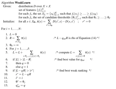
The pseudocode for the weak learner is given in Figure 3. Note that the input to the algorithm in-cludes for each feature a sorted list of candidate thresholds_{θj}Jj=1for that feature. For convenience

we assume thatθ1=∞andθJ=−∞. Also, the value|r| is calculated according to Equation (14):

the variable L stores the left summand and the variable R stores the right summand. Finally, if the default rank qdefis specified by the user, then step 6 is skipped.

Thus, for a given ranking feature, the total time required to evaluate|r|for all candidate weak rankings is only linear in the number of instances that are ranked by that feature. In summary, we have shown the following theorem:

Theorem 2 The algorithm of Figure 3 finds the weak ranking of the form given in Equation (9) that maximizes_|r_|as in Equation (10). The running time is O(n_|Φ_||

X

Φ|)per round of boosting. An efficient implementation runs in time

O _|Φ_|+

n

∑

i=1 |

X

fi|

!

=O(_|Φ_|+n_|

X

Φ|).

(15)

Algorithm WeakLearn

Given: distribution D overX_×X set of features_{fi}N_i₌₁

for each fi, the setXfi={xk}

K

k=1such that fi(x1)≥. . .≥fi(xK)

for each fi, the set of candidate thresholds{θj}J_j₌₁such thatθ1≥. . .≥θJ

Initialize: for all x_∈X_Φ,π(x) =

∑

x0_∈_X_Φ

D(x0,x)−D(x,x0) ; r∗=0

For i=1, . . . ,N:

1. L=0 2. R=

∑

x∈X_fi

π(x) /* L₋qdefR is rhs of Equation (14) */

3. θ0=∞

4. For j=1, . . . ,J:

5. L=L+

∑

x:θj−1≥fi(x)>θj

π(x) /* compute L=

∑

x: fi(x)>θ

π(x) */

6. if_|L_|>|L₋R_| /* find best value for qdef */ 7. then q=0

8. else q=1

9. if_|L₋q R_|>|r∗_| /* find best weak ranking */ 10. r∗=L₋q R

11. i∗=i 12. θ∗=θj

13. q∗def=q

Output weak ranking(fi∗,θ∗,q∗def)

Figure 3: The weak learner.

Positive cumulative weights. Since the final ranking has the form H(x) =∑T

t=1αtht(x)and the

rankings output by WeakLearn are binary, if ht(x) =1 then ht contributes its weightαt to the final

score of x. During the boosting process, WeakLearn may output distinct rankings that correspond to different thresholds of the same feature f . If we view these rankings in increasing order by threshold, we see that f ’s contribution to the final score of x is the sum of the weights of the rankings whose thresholds are less than f(x). To simplify matters, if we assume that ht occurs exactly once among

h1, . . . ,hT, then if the weightsαt are always positive, then f ’s contribution increases monotonically

with the score it assigns instances.

This behavior of a feature’s contribution being positively correlated with the score it assigns is desirable in some applications. In the meta-search task, it is natural that the search strategy f should contribute more weight to the final score of those instances that appear higher on its ranked list. Put another way, it would seem strange if, for example, f contributed more weight to instances in the middle of its list and less to those at either end, as would be the case if some of theαt’s were

negative. Also, from the perspective of generalization error, if we allow someαt’s to be negative

then we can construct arbitrary functions of the instance space by thresholding a single feature, and this is probably more complexity than we would like to allow in the combined ranking (in order to avoid overfitting). In summary, while RankBoost may set someαt’s to be negative, we developed an

alternative version that enforces the constraint that all of the values ofαt’s are positive. Thus, each

(16)

To address this situation, we implemented an additional version of WeakLearn that chooses its rankings to exhibit this monotonic behavior. In practice, our earlier assumption that all ht’s

are unique may not hold. If it does not, then the contribution of a particular ranking h will be

its cumulative weight, the sum of those αt’s for which ht =h. Thus we need to ensure that this

cumulative weight is positive. Our implementation outputs the ranking that maximizes_|r_|subject to the constraint that the cumulative weight of that ranking remains positive. We refer to this modified weak learner as WeakLearn.cum.

5. Generalization Error

In this section, we derive a bound on the generalization error of the combined ranking when the weak rankings are binary functions and the feedback is bipartite. That is, we assume that the feedback partitions the instance space

X

into two disjoint sets, X and Y , such thatΦ(x,y)>0 for all x∈X and y_∈Y , meaning the instances in Y are ranked above those in X . Many problems can be viewed as

providing bipartite feedback, including the meta-search and movie recommendation tasks described in Section 6, as well as many of the problems in information retrieval (Salton, 1989, Salton and McGill, 1983).

5.1 Probabilistic Model

Up to this point we have not discussed where our training and test data come from. The usual as-sumption of machine learning is that there exists a fixed and unknown distribution over the instance space. The training set (and test set) is a set of independent samples according to this distribution. This model clearly translates to the classification setting where the goal is to predict the class of an instance. The training set consists of an independent sample of instances where each instance is labeled with its correct class. A learning algorithm formulates a classification rule after running on the training set, and the rule is evaluated on the test set, which is a separate independent sample of unlabeled instances.

This probabilistic model does not translate as readily to the ranking setting, however, where the goal is to predict the order of a pair of instances. A natural approach for the bipartite case would be to assume a fixed and unknown distribution D over

X

_×

X

, pairs from the instance space.4 The obvious next step would be to declare the training set to be a collection of instances sampled independently at random according to D. The generalization results for classification would then trivially extend to ranking. The problem is that the pairs in the training set are not independent: if (x1,y1)and(x2,y2)are in the training set, then so are(x1,y2)and(x2,y1).

Here we present a revised approach that permits sampling independence assumptions. Rather than a single distribution D, we assume the existence of two distributions, D0over X and D1over Y .

The training instances are the union of an independent sample according to D0and an independent

sample according to D1. (This is similar to the “two button” learning model in classification, as

describe by Haussler et al. 1991.) The training set, then, consists of all pairs of training instances. Consider the movie recommendation task as an example of this model. The model suggests that movies viewed by a person can be partitioned into an independent sample of good movies and an independent sample of bad movies. This assumption is not entirely true since people usually choose

4. Note that assuming a distribution over X×Y trivializes the ranking problem: the rule which always ranks the second

(17)

which movies to view based on movies they’ve seen. However, such independence assumptions are common in machine learning.

5.2 Sampling Error Definitions

Given this probabilistic model of the ranking problem, we can now define generalization error. The final ranking output by RankBoost has the form

H(x) =

T

∑

t=1

αtht(x)

and orders instances according to the scores it assigns them. We are concerned here with the

pre-dictions of such rankings on pairs of instances, so we consider rankings of the form H :

X

_×

X

_→

{−1,0,+1}, where

H(x,y) =sign

T

∑

t=1

αtht(y)− T

∑

t=1

αtht(x)

!

(15)

where the ht come from some class of binary functions

H

. Let

C

be the set of all such functions H.

A function H misorders(x,y)_∈X_×Y if H(x,y)₆=1, which leads us to define the generalization error of H as

ε(H) = Prx_∼D0,y∼D1[H(x,y)6=1]

= ED0,D1[[[H(x,y)6=1]]] .

We first verify that this definition is consistent with our notion of test error. For a given test sample

T0×T1where T0=hx1, . . . ,xpiand T1=

y1, . . . ,yq

, the expected test error of H is

ET0,T1

"

1

pq

∑

_i_,_j[[H(xi,yj)6=1]]

#

= 1

pq

∑

_i_,_jET0,T1[[[H(xi,yj)6=1]]]

= 1

pq

∑

_i_,_jPrxi,yj[H(xi,yj)6=1]

= 1

pq

∑

_i_,_jε(H) =ε(H).

Similarly, if we have a training sample S0×S1where S0=hx1, . . . ,xmiand S1=hy1, . . . ,yni, the

training (or empirical) error of H is

ˆ

ε(H) = 1

mn

∑

_i_,_j[[H(xi,yj)6=1]].

(18)

5.3 VC Analysis

We now bound the difference between the training error and test error of the combined ranking out-put by RankBoost using standard VC-dimension analysis techniques (Devroye et al., 1996, Vapnik, 1982). We will show that, with high probability taken over the choice of training set, this difference

is small for every H_∈

C

. If this happens then no matter which combined ranking is chosen by

our algorithm, the training error of the combined ranking will accurately estimate its generalization

error. Another way of saying this is as follows. Let Z denote the event that there exists an H_∈

C

such that ˆε(H)andε(H)differ by more than a small specified amount. Then, the probability (over the choice of training set) of the event Z is very small. Formally, we will show that for everyδ>0, there exists a smallεsuch that

PrS0∼Dm0,S1∼Dn1

"

∃H_∈

C

:

1

mn

∑

_i_,_j[[H(xi,yj)6=1]]−Ex,y[[[H(x,y)6=1]]]

>ε #

≤δ (16)

where the choice ofεwill be determined during the course of the proof.

Our approach will be to separate (16) into two probabilities, one over the choice of S0 and the

other over the choice of S1, and then to bound each of these using classification generalization error

theorems. In order to use these theorems, we will need to convert H into a binary function. Define

F : X_×Y_{→ {}0,1_}as a function which indicates whether or not H misorders the pair(x,y), meaning

F(x,y) = [[H(x,y)₆=1]]. Although H is a function on

X

_×

X

, we only care about its performance on pairs(x,y)_∈X_×Y , which is to say that it incurs no penalty for its ordering of two instances from

ybe the set of all such functions F for a fixed y. Then the choice of F in (20) comes

fromS

y

F

y. A theorem of Vapnik (1982) applies to (20) and gives a choice ofε0 that depends on

the size m of the training set S0, the error probabilityδ, and the complexity d0ofSy

F

y, measured as

its VC-dimension (for details, see Vapnik 1982 or Devroye et al. 1996). Specifically, for anyδ>0,

PrS0∼Dm0

"

∃F_∈[

F

y :

1

m

∑

>ε0(m,δ,d0)

#

<δ,

where

ε0(m,δ,d0) =2

r

d0(ln(2m/d0) +1) +ln(9/δ)

m .

The parameters m andδare given; it remains to calculate d0, the VC-dimension ofS

y

F

y. (We note

that although we are using a classification result to bound (20), the probability corresponds to a peculiar classification problem (trying to differentiate X from Y by picking an F and one y_∈Y ) that

does not seem to have a natural interpretation.)

Let’s determine the form of the functions inS

y

F

y. For a fixed y∈Y ,

F(x,y) = [[H(x,y)₆=1]]

= ""

sign

T

∑

t=1

αtht(y)− T

∑

t=1

αtht(x)

! 6 =1 ## = "" T

∑

t=1

αtht(x)− T

∑

t=1

αtht(y)≥0

##

= ""

T

∑

t=1

αtht(x)−b≥0

##

where b=∑T_t₌₁αtht(y)is constant because y is fixed. So the functions inSy

F

y are a subset of all

possible thresholds of all linear combinations of T weak rankings. Freund and Schapire’s (1997) Theorem 8 bounds the VC-dimension of this class in terms of T and the VC-dimension of the weak

ranking class

H

. Applying their result, we have that if

H

has VC-dimension d_≥2, then d0 is at

most

2(d+1)(T+1)log₂(e(T+1)) ,

where e is the base of the natural logarithm.

As the final step, repeating the same reasoning for (19) keeping x fixed, and putting it all to-gether, we have thus proved the main result of this section:

Theorem 3 Let

C

be the set of all functions of the form given in Eq (15) where all the ht’s belong

to a class

H

of VC-dimension d. Let S0and S1be samples of size m and n, respectively. Then with probability at least 1₋δover the choice of training sample, all H_∈

C

satisfy

|εˆ(H)₋ε(H)_{| ≤}2

r

d0₍_ln₍_2m_/_d0_{) +}₁_{) +}_ln₍₁₈_/δ₎

m +2

r

d0₍_ln₍_2n_/_d0_{) +}₁_{) +}_ln₍₁₈_/δ₎

n ,

(20)

6. Experimental Evaluation of RankBoost

In this section, we report experiments with RankBoost on two ranking problems. The first is a sim-plified web meta-search task, the goal of which is to build a search strategy for finding homepages of machine-learning researchers and universities. The second task is a collaborative-filtering problem of making movie recommendations for a new user based on the preferences of other users.

In each experiment, we divided the available data into training data and test data, ran each algorithm on the training data, and evaluated the output ranking on the test data. Details are given below.

6.1 Meta-search

We first present experiments on learning to combine the results of several web searches. This problem exhibits many facets that require a general approach such as ours. For instance, approaches that combine similarity scores are not applicable since the similarity scores of web search engines often have different semantics or are unavailable.

6.1.1 DESCRIPTION OFTASK ANDDATASET

Most of the details of this dataset and how we mapped it into the general ranking framework were described in Section 2.1.

Given this mapping of the ranking problem into our framework, we can immediately apply RankBoost. Note that the feedback function for this problem is a sum of bipartite feedback functions so the more efficient implementation described in Section 3.3 can be used.

Under this mapping, each weak ranking is defined by a search template i (corresponding to ranking feature fi), and a threshold valueθ. Given a base query q and a URL u, this weak ranking

outputs 1 or 0 if u is ranked above or below the threshold θ on the list of URLs returned by the

expanded query associated with search template i applied to base query q. As usual, the final ranking H is a weighted sum of the weak rankings.

For evaluation, we divided the data into training and test sets using four-fold cross-validation. We created four partitions of the data, each one using 75% of the base queries for training and 25% for testing. Of course, the learning algorithms had no access to the test data during training.

6.1.2 EXPERIMENTAL PARAMETERS ANDEVALUATION

Since all search templates had access to the same set of documents, if a URL was not returned in the top 30 documents by a search template, we interpreted this as ranking the URL below all of the

returned documents. Thus we set the parameter qdef, the default value for weak rankings, to be 0

(see Section 4).

Our implementation of RankBoost used a definition of ranking loss modified from the original given in Section 2, Equation (1):

rlossD(H) =

∑

x0,x1

D(x0,x1) [[H(x1)≤H(x0)]] .

If the output ranking ranked as equal a pair(x0,x1)of instances that the feedback ranked as unequal,

(21)

0 0.005 0.01 0.015 0.02 0.025 0.03 0.035

20 40 60 80 100 120 140 160 180 200

Train Error

Rounds of Boosting WeakLearn.2 WeakLearn.2.cum WeakLearn.3 WeakLearn.3.cum

0.02 0.025 0.03 0.035 0.04 0.045 0.05 0.055

20 40 60 80 100 120 140 160 180 200

Test Error

Rounds of Boosting WeakLearn.2 WeakLearn.2.cum WeakLearn.3 WeakLearn.3.cum

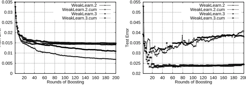
Figure 4: Performance of the four weak learners WeakLearn._{2,3,2.cum,3.cum_}on the ML dataset.

Left: Train error Right: Test error

(x0,x1)is 1/2, since the probability that x0 is listed above x1 is equal to the probability that x1 is

listed above x0. The modified definition is

rlossD(H) =

∑

x0,x1

D(x0,x1) [[H(x1)<H(x0)]] +1₂

∑

x0,x1

D(x0,x1) [[H(x1) =H(x0)]] . (21)

RankBoost parameters. Since WeakLearn outputs binary weak rankings, we can set the parame-terαusing either the second or third methods presented in Section 3.2. The second method setsαas

the minimum of Z, and the third method setsαto approximately minimize Z. The third method can

be implemented more easily and runs faster. We implemented both methods, called WeakLearn.2 and WeakLearn.3, to determine if the extra time required by the second method (almost ten times that of the third method on the ML dataset) was made up for by a reduction in test error rate. We also implemented weak learners that restricted their rankings to have positive cumulative weights in order to test whether such rankings were helpful or harmful in reducing test error (as discussed at the end of Section 4). We called these WeakLearn.2.cum and WeakLearn.3.cum.

To measure the accuracy of a weak learner on a given dataset, after each round of boosting we plotted the train and test error of the combined ranking generated thus far. We ran each weak learner for 1000 rounds of boosting on each of the four partitions of the data and averaged the results. Figure 4 displays the plots of train error (left) and test error (right) for the first 200 rounds of boosting on the ML dataset. (The slopes of the curves did not change during the remaining 800 rounds.) The plots for the UNIV dataset were similar.

WeakLearn.2 achieved the lowest train error, followed by WeakLearn.3, and finally Learn.2.cum and WeakLearn.3.cum, whose performance was nearly identical. However, Weak-Learn.2.cum and WeakLearn.3.cum produced the lowest test error (again behaving nearly identi-cally) and resisted overfitting, unlike their counterparts. So we see that restricting the weak rankings to have positive cumulative weights hampers training performance but improves test performance. Also, when we subject the rankings to this restriction, we see no difference between the second

and third methods of settingα. Therefore, in our experiments we used WeakLearn.3.cum, the third