Published online January 31, 2015 (http://www.sciencepublishinggroup.com/j/pamj) doi: 10.11648/j.pamj.20150401.14
ISSN: 2326-9790 (Print); ISSN: 2326-9812 (Online)
On the Accelerated Overrelaxation Method
I. K. Youssef
1, M. M. Farid
21
Math. Dept. Faculty of Science Ain Shams Uni., Cairo, Egypt 2
Basic Science Dept. British University in Egypt, Elshorouk City, Cairo, Egypt
Email address:
[email protected] (I. K. Youssef), [email protected] (M. M. Farid)
To cite this article:
I. K. Youssef, M. M. Farid. On the Accelerated Overrelaxation Method. Pure and Applied Mathematics Journal. Vol. 4, No. 1, 2015, pp. 26-31. doi: 10.11648/j.pamj.20150401.14
Abstract:
A new variant of the accelerated over relaxation (AOR) method for solving systems of linear algebraic equations, the KAOR method is established. The treatment depends on the use of the extrapolation techniques introduced by Hadjidimos (1978) and the KSOR introduced by Youssef (2012) and its modified version published in (2013). The KAOR is an extrapolation version of the KSOR. This approach has enables us in establishing eigenvalue functional relations concerning the eigenvalues of the iteration matrices and their spectral radii. Moreover, our eigenvalue functional relation depends directly on the eigenvalues of Jacobi iteration matrix. The proposed method considers the advantages of the AOR in addition to those of the KSOR. A graphical representation of the behavior of the spectral radius near the minimum value illustrates the smoothness in the choice of optimum parameters.Keywords:
SOR, KSOR, AOR, QAOR, KAOR1. Introduction
Consider a linear system of algebraic equations of the form
AX = b
(1)n n
R
A
∈
× with non-vanishing diagonal elements. It is generally, accepted that the matrix of coefficients can be written in the formU
L A
A
A=D− − (2)
Where D is the diagonal part of the matrix
A
andA
L andU
A
are the strictly lower and upper triangular parts of the matrixA
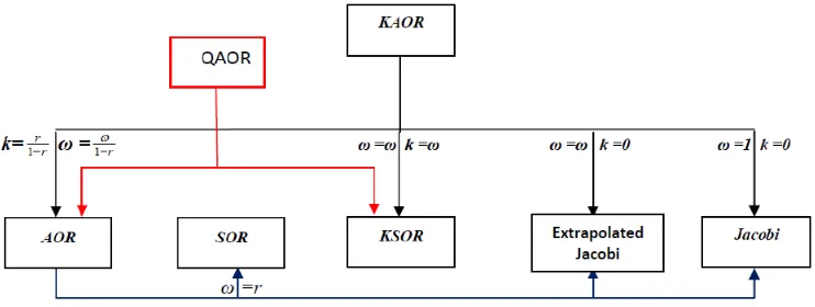
, respectively. Hadjidemose, [1] in 1978 introduced the accelerated overrelaxation iterative method (AOR) as a two parameter generalization of the standard Jacobi, Gauss- seidel, and successive overrelaxation (SOR) methods, [2, 3] as shown figure (1) ,It is common to normalize the system (1) such that the diagonal elements are all equal one in this case the matrix of coefficients
A
is written asU L A=I− −
Accordingly, the AOR method can be written in the form
b rL I X
L
X[n+1]= r,ω [n] +ω( − )−1
(
) (
)
[
I r L U]
rL I
Lr,ω=( − )−1 1−ω + ω− +ω
Moreover, the (AOR) can be seen as an extrapolation of (SOR) method with overrelaxation parameter r and extrapolation parameter s=ω/r, [4, 5].
Youssef [6] in 2012, introduced the KSOR as a new variant of the SOR, Youssef and Taha [7] in 2013 introduced the modified versions of the KSOR, the main idea of the KSOR is the assumption of using the current component in the updating process instead of using the most recent calculated values in the SOR methods. The KAOR method is introduced as a new variant of the AOR method. The KAOR can be introduced through two equivalent treatment of the KSOR approach the first is the interpolation process in terms of the sub-matrices as in Hadjidemose, [1] and the second is the extrapolation of the KSOR method. The second approach confirms the first and moreover facilitates the treatment in establishing eigenvalue functional relation, [4, 5].
2. The KAOR Method
the coefficient of the new iterate is an at most lower triangular matrix is
b +a )X A +a A D + a = (a ) X A D + a
(a1 2 L n+1 3 4 L 5 U n 6 ,
⋯ , 1 , 0
=
n (3)
as in Hadjedemos [1],
where
a
i,i =
1
(
1
)
6
are constants to be determined. Sufficient conditions for scheme (3) to be consistent with Eq. (1) are0
6 6 54 2 3
1
- a
)D + (a
- a
)A
- a
A
= a
A,
a
(a
L U≠
(4)In view of (2), the first relation of (4) gives
6 5 6
4 2 6 3
1
- a
= a
, a
- a
=- a
and -
a
= - a
a
The above set of equations has the following two- parameter solution
ω ω
ω , a = k and a = a = + k
= a k , = , a = k+
a1 1 2 − 3 1 − 4 − 5 6 ,
where k and ω ≠ 0 are fixed parameters. Consequently, (3) becomes
C + x U L + k I + k = x k L I
k+1) ) (n+ ) [( ω) (ω ) ω ] n ω
(( − 1 − − ,
⋯ , 1 , 0
=
n (5)
where we have
b
D
, C =
A
D
, U =
A
L = D
-1 L -1 U -1 (6)and I the identity matrix of order N. The form (5) is the KAOR method or Mk,ω -method. We observe that for specific
values of the parameters k and ω, theMk,ω-method reduces to
well-known methods. Thus
M0,1-method is the Jacobi method,
M0,ω-method is the extrapolated Jacobi method,
Mω,ω-method is the KSOR method.
Now we will use the notations Lk,ω for the iteration matrix
of the method in (5),
U] k)L + I +
+k [ k L I k+ =
Lk,ω (( 1) − )−1 (1 −ω) (ω− ω ρ(Lk,ω) is the spectral radius of Lk,ω.
It should be noted that, except for the case, ω= 0, the
KAOR method is essentially the Extrapolated (E)KSOR method with overrelaxation parameter k and extrapolation one s =ω/k, for it is easy to show that
- s)I + ( = sL Lk,ω k,k 1
Thus if v is an eigenvalue of Lk,k (k ≠ 0) and λ, the
corresponding one of Lk,ω , we have that
)
1
(
- s
λ = sν +
(7)By considering the KAOR method as an extrapolation of the KSOR method, we can use the extrapolation theorem in the evaluations of the possible values of the parameters k and ω for the KAOR method.
Extrapolation Theorem
If the scheme [xn+1=Txn+c] converges [ρ(T)<1] and ]
( 1 [ 2
0<ω< / + ρT ) , then the extrapolated scheme [xn+1 =[(1−ω)I +ωT]xn+ωC ]converges.
Proof, [4].
Theorem 1: the domain of convergence of the relaxation parameter of the KSOR method can be written in the form ω∈R−[−2,0], [6].
Theorem 2: the sufficient conditions for KAOR to converge
1) for k ]0, [∈ ∞ , is 0<ω<2k/[1 + ρ(Lk,k )] 2) for k ]∈ − ∞ −, 2[, is 2k/[1 + ρ(Lk,k )]<ω<0
Proof, (1) for k∈ ∞]0, [ , from Theorem1 the KSOR converges, and from Extrapolation Theorem the KAOR method converges for 0<ω/k<2/[1 + ρ(Lk,k )]where (ω/k) is the extra- polation parameter , and where k is positive then the condition is 0<ω<2k/[1 + ρ(Lk,k )].
(2)for k
∈
]
−
∞
,
−
2
[
, by the same way of (1), but where k is negative and the condition will be2k/[1 + ρ(Lk,k)]< ω < 0.
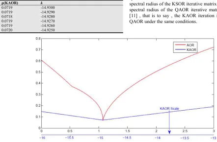
Here we can say that the KAOR method extends the range for choosing the parameters k and ω which reduce the sensitive of the spectral radius of the iteration matrix with the changes in k and ω like the KSOR method, as shown in figure (2).
The discussion of the AOR for general linear systems is very complicated so the publications have considered the practical cases, [8, 9, 10] like irreducible matrices with weak diagonal dominance, L matrices and the consistently ordered matrices.
Figure 1. A diagram for the relative comparison for QAOR, KSOR, AOR and KAOR.
3. Irreducible and
L
Matrices
Because of the difficulty in the general treatment, we consider two important cases, the case of irreducible matrix with weak diagonal dominance and the L matrix case.
3.1. Irreducible Matrices with Weak Diagonal Dominance
It is known that if A is an irreducible matrix with weak diagonal dominance, then it will be nonsingular with non-vanishing diagonal elements.
Theorem.If A is an irreducible matrix with weak diagonal dominance, then the Mk,ω-method converges for all0 < k and
0 < ω.
Proof. We assume that for some eigenvalue λ of Lk,ωwe
have |λ| > 1. For this eigenvalue the relationship below holds det(Lk,ω -λI) = 0 (8)
or after performing simple series of transformations
det(Q) = 0, (9)
Where we have
U ) +k)(λ ω+(
ω L
) +k)(λ ω+(
)) +k(λ ( Q=I
1 1
1 1
1
− −
− −
− ω (10)
The coefficients of L and U in (10) are less than one in modulus. To prove this it is sufficient and necessary to prove that
|
1)
-k(
+
|
|
1)
-k)(
+
(1
+
|
ω
λ
≥
ω
λ
and,|
|
|
1)
-k)(
+
(1
+
|
ω
λ
≥
ω
(11)If λ-1 = qeiθ where q and θ are real with 0 < q < 1, then the first inequality in (11) is equivalent to
2 2
1 2+ k + q + q (k2 −ω)−2q( + k)( + k1 1 −ω)cosθ+ qk(k2 −ω)cosθ≥0 (12)
Since the expression in the brackets above is nonnegative, (12) holds for all real θ if and only if it holds for cosθ = 1. Thus, (12) is equivalent to
0
1
2
1
2
1
2
1
−
q)
2+
k(
−
q)+
q
(
−
q)+
qk(q
−
)
≥
(
ω
(13)for q = 1; otherwise it is equivalent to
0
1
2
1
2
1
−
q)
2+
k(
−
q)
2+
q
(
−
q)
≥
(
ω
(14)Which is true.
The second inequality in (11) is equivalent to
0 cos ) 1 )( 1 ( 2 ) 1 ( 2 ) 1 ( ) 1
(+k 2+q2 +k 2− q2ω +k − q +k +k−ω θ ≥ Which, for the same reason, must be satisfied for
1
cosθ= .thus, we have
2
2 2 2 2
(1+ k) + q (1+ k) −2q ω( + k1 )−2 (1q + k) + q2 ω(1+ k)≥0
Or equivalent to
[(1+k) – q(1+k)]2+2qω(1+k) (1 –q) ≥ 0,
which is also true.
Since A has weak diagonal dominance and is irreducible it is obvious that
D
−1A=I
−
L
−
U
preserves the same properties. The same is true for the matrix Q since the coefficients of L and U are different from zero and less than one in modulus. Thus, Q is nonsingular which contradicts (9) and, consequently, (8). Therefore ρ(Lk,ω) < 1.Considering now the Mk,ω-methods corresponding to the
pairs (k, ω)=(0,1), (0,ω)and (ω,ω) we can write the following corollary
Corollary.If A is an irreducible matrix with weak diagonal dominance, then the methods of Jacobi, extrapolated Jacobi and KSOR converge.
3.2. L-Matrices
If Ais an L-matrix that is a matrix whose elementsaij ,
i,j = 1(1 )N satisfy the relationships
)N ( j, i, j = i
< a )N and (
i= >
aii 0, 11 ij 0, ≠ 11
then the following theorem concerning the KAOR method can be proved.
THEOREM If A is an L-matrix, then for all k and ω such that 0 <k < ω < k+1 (ω ≠ 0) the Mk,ω-method converges if
Proof. It is obvious that if the Mk,ω-method converges so
does the M0,1-method. Assume now that λ = ρ(Lk,ω) > 1.
Because of our assumptions we easily get that
0 1+ k− )I + ( −k)L + U] ≥
[( ω ω ω
and also that
1 1 2 2 1 1
[ 1 ] [ ] 0
1 1 1 1
n
n-k k k
(k + )I - kL I +( )L +( ) L + +( ) L
( + k) k + k + k +
− = − ≥
⋯
thus, for the iteration matrix we have that
0 ] ( ) 1 [( 1 ) ) 1
((k+ I−k L− +k− I + −k)L + U ≥ =
k,
L ω ω ω ω
Since Lk,ω is a nonnegative matrix, λ is an eigenvalue of
Lk,ω . If V≠ 0 is the corresponding eigenvector, we have Lk,ω
V= λ V from which we can obtain that
V k V U L k ω ω λ ωλ
ω+ − + =(1+ )( −1)+
) ) 1 ( (
This implies that
ω ω λ− + + )( 1) 1
( k
is an eigenvalue of
) ) 1 (
( +k − L+U
ωλ ω . Therefore ) ) 1 ( ( ) 1 )( 1 ( U L k
k − + ≤ + − +
+ ωλ ω ρ ω ω λ
It is obvious that + ( −1)≥1
ωλ ω k so that ) ( ) 1 ( ) 1 (
0≤ +k − L+U≤ +k − L+U
ωλ ω ωλ ω 1 , 0 ) 1 ( L k ω λ
ω+ −
= Then ) ( )) 1 ( ( ) 1 )( 1
( +k λ− +ω≤ ω+k λ− ρ L0,1
from which we can easily obtain that ρ(L1,0) ≥ 1. Since we
have proved that if λ≥1, then ρ(L1,0)> 1, we can readily
obtain that ρ(L1,0) < 1 implies λ<1 so that if the M1,0
-method converges then so does the Mk,ω-method. 3.3. Consistently Ordered Matrices
In this section we assume that matrix A is a consistently ordered one, that is, a matrix for which the expression det (aAL+ a-1Au - bD) is independent of a for a ≠ 0 and for all b.
As can be easily found out, the analysis of this section also applies in the case where A is a matrix which has property A. LEMMA. If A is a consistently ordered matrix with non-vanishing diagonal elements, and if µ≠0 is an eigenvalue of L1,0of multiplicity p, then -µ is also an eigenvalue of L1,0of
multiplicity p.
Proof. See Theorems 3.4 and 2.2 on pages 147 and 142, respectively, of Young [2].
THEOREM. If A is a consistently ordered matrix with non-vanishing diagonal elements, and if µ is an eigenvalue of L1,0
and v satisfies
2 2 2 ) 1
(ν+νω− =νµ ω (15) Then v is an eigenvalue of Lω,ω and vice versa.
Proof. See [6]
THEOREM. If A is a consistently ordered matrix with non-vanishing diagonal elements, and if µ is an eigenvalue of L1,0 and λ satisfies
] ) 1 ( [ )] 1 ( ) 1
[(k+ λ− +k−ω 2=µ2ωk λ− +ω (16) then λ is an eigenvalue of Lk,ω and vice versa.
Proof. Since the requirements of theorem 1 are fulfilled, for ω≠0, we substitute the value of ν in terms of λ from (7) into (15) and its equivalent relationship (16) follows. For ω= 0 it is easy to show that, λ satisfies (16) and vice versa.
THEOREM. If A is a consistently ordered matrix with non-vanishing diagonal elements, and if L1,0 has real eigenvalues µi ,|i=1(1)N such that, 0 < mini|µi|=maxi|µi|<1,
then for )
2 2 / 1 ) 2 1 ( 1 ( 2 , ) 2 2 / 1 ) 2 1 ( 1 ( 2 ) 2 2 / 1 ) 2 1 ( 2 2 )( 2 / 1 ) 2 1 ( 1 ( ( µ µ µ µ µ µ µ µ
ω − + −
+ − − − + − − − − + − ) = (k,
Or )
) 2 / 1 ) 2 1 ( 1 ( 2 , ) 2 2 2 2 / 1 ) 2 1 ( 2 2 / 1 ) 2 1 ( 2 ( 2 ) 2 / 1 ) 2 1 ( 2 2 2 ( (
2 µ µ µ µ µ
µ µ µ − + − + − − + − − − + − − ,
ρ(Lk,ω) = 0.
Proof. From the Lemma, µ will be an eigenvalue of L0,1.
Sinceµ2assumes one and only one fixed value we can derive values for ω≠0 so that (15) has a double root.
These values are
) 2 / 1 ) 2 1 ( 1 ( 2 2 , 2 2 / 1 ) 2 1 ( 1 ( 2 1 µ ω µ µ ω − + − = − + −
= (17)
and the double root for v will be given by
2 ) 1 ( 2 2 2 ) 1 ( 2 ω ω µ ω ν + + +
= (18)
Since ν has only one value it is easy to determine s (i.e. k) from (1.7) so that λ = 0. For this we must have
k =ω/(l –ν ) (19)
Thus we finally obtain
) 2 2 / 1 ) 2 1 ( 1 ( 2 ) 2 2 / 1 ) 2 1 ( 2 2 )( 2 / 1 ) 2 1 ( 1 ( 1 µ µ µ µ µ µ + − − − + − − − − + − = k ) 2 2 2 2 / 1 ) 2 1 ( 2 2 / 1 ) 2 1 ( 2 ( 2 ) 2 / 1 ) 2 1 ( 2 2 2 ( 2
2 − − + − − +
− + − − = µ µ µ µ µ µ µ
k (20)
The pairs (k1,ω1) and (k2, ω2) give ρ(Lk,ω) = 0 .
4. Numerical Examples
sensitivity of the relaxation parameter is considerably relaxed in the KAOR in comparison with the AOR as in the KSOR in comparison with the SOR [6], figure (2) below illustrates this behavior. The range of the relaxation parameters is extended as in the KSOR (R-[-2, 0]) as shown in table 3, which is ignored in the so called QAOR [11].
Example 1 consider the matrix [8]
1 1
5 5
18 5 24 1
5 5
12 1
5 5
1 0
0 1 6
1 0
0 1
−
the eigenvalues of the Jacobi matrix are
±
24
/
5
, each one with multiplicity two. Thus 0 < µ =24
/
5
=µ
< 1Since the restrictions of Theorem 3 are satisfied, the corresponding values for the KAOR method are (k1, ω1) =
(-15/2, -5/2) and (k2, ω2) = (10/3, -5/3), where both pairs give
ρ(Lk,ω) = 0, as it was in the AOR. Example 2 Consider the system [6]
=
− −
− −
− −
− −
=
1 1 1 1 , 4 1 1 0
1 4 0 1
1 0 4 1
0 1 1 4
b A
Table 1. The behavior of the spectral radius ρ(KAOR)near the minimum
value.
ρ(KAOR) k
0.0719 -14.9300 0.0719 -14.9290 0.0718 -14.9280 0.0719 -14.9270 0.0719 -14.9260 0.0720 -14.9250
Table 2. the behavior of the spectral radius of KAOR near the minimum
value.
ρ(AOR) r
0.0927 1.0700
0.0858 1.0710
0.0722 1.0720
0.0740 1.0730
0.0758 1.0740
0.0775 1.0750
The behavior of thespectral radius of the KAOR iteration matrix is very smooth than the behavior of spectral radius of the AOR iteration matrix around the optimum eigenvalue see figure (2).
Example 3 Consider the system [11]
1 1
ij 10 20
1 1
ij 10( ) 20
,
1,
,
j
ii
i j
a i j
A a
a − i j
= − >
= =
= − <
Table 3.ρ(KSOR) and ρ(KAOR).
n ω(KSOR) k ω(KAOR) ρ(KSOR) ρ(KAOR)
8 -17.85 -16.3 -16.2 0.13537756 0.13537172
16 -7.82 -11.9 -12.5 0.240810 0.240495
20 -3.6 -3 -2.5 0.49703 0.39082
As we see in the table 3: where n is the size of A, the spectral radius of the KAOR iterative matrix is less than spectral radius of the KSOR iterative matrix and less than the spectral radius of the QAOR iterative matrix introduced in [11] , that is to say , the KAOR iteration is faster than the QAOR under the same conditions.
5. Conclusion
The KAOR is an extrapolation version of the KSOR similar to the situation in the AOR with the SOR. As in the AOR, the KAOR reduces to well-known methods at specific values of the parameters κ, ω like the Jacobi, extrapolated Jacobi and the KSOR. In comparison with the AOR the KAOR preserves the properties of the KSOR, the behavior of spectral radius is relaxed near the optimum values, figure 2.
It is noticed that some recent publication [11] has ignored the negative values of the relaxation parameters in spite of their high importance as we have seen the optimum values occurs in this part of the domain.
Shi-liang Wu, Yu-Jaun Liu [11], introduced the QAOR as a generalization of the KSOR from the AOR point of view, their relational graph figure 1 illustrates that The QAOR is ageneralization of the KSOR (ω=r) but it is not an extrapolation version as the situation in the AOR and the SOR. Moreover, as shown in the relational graph the KAOR
generalizes, the AOR (
r r
r k
− = − =
1 , 1
ω
ω ), and generalizes
the KSOR (ω=k), generalizes the Jacobi (ω =1, k=0) and the extrapolated Jacobi (k=0 ).
References
[1] A. Hadjidimos, Accelerated Overelaxation Method, Math. Comput. , 32, pp149-157, 1978.
[2] D.M. Young, Iterative Solution of Large Linear Systems, Academic Press, New York, 1971.
[3] R.S. Varga, Matrix Iterative Analysis, prentice-Hall, Englewood cliffs, N. J., 1962.
[4] A. Hadjidimos, A. Yeyios, The Principale of Extrapolation in Connection With the Accelerated Overrelaxation Method, Linear Algebra and its Applications 30, 115-128 , 1980. [5] N. M. Missirlis, D. J. Evans, The Extrapolated Successive
Overrelaxation (ESOR) Method for Consistently Ordered Matrices, Internat. J. Math. & Math. sci. Vol. 7, No. 2, pp. 361-370, 1984.
[6] I.K. Youssef, On the Successive Overrelaxation method, J. Math. Stat., 8 pp.176-184, 2012.
[7] I.K. Youssef, A.A. Taha, On the Modified Successive Overrelaxation Method, Appl. Math.Comput., 219, pp. 4601-4613, 2013.
[8] G. Avdelas and A. Hadjidimos, Optimum Accelerated Overrelaxation Method in a Special Case, Mathematics of computation Vol. 36, No. 153, 1981.
[9] M. Madalena Martins, On an Accelerated Over relaxation Iterative Method for Linear Systems With Strictly Diagonally Dominant Matrix, Mathematics of Computation, Vol. 35, No. 152, pp. 1269-1273, 1980.
[10] A.J. Hughes Hallet, The Convergence of Accelerated Overrelaxation Iterations, Mathematics of Computation, Vol. 47, No. 175, pp. 219-223, 1986.