Transfer in Reinforcement Learning via Shared Features
George Konidaris [email protected]
Computer Science and Artificial Intelligence Laboratory Massachusetts Institute of Technology
32 Vassar Street Cambridge MA 02139
Ilya Scheidwasser [email protected]
Department of Mathematics Northeastern University 360 Huntington Avenue Boston MA 02115
Andrew G. Barto [email protected]
Department of Computer Science University of Massachusetts Amherst 140 Governors Drive
Amherst MA 01003
Editor: Ronald Parr
Abstract
We present a framework for transfer in reinforcement learning based on the idea that related tasks share some common features, and that transfer can be achieved via those shared features. The framework attempts to capture the notion of tasks that are related but distinct, and provides some insight into when transfer can be usefully applied to a problem sequence and when it cannot. We apply the framework to the knowledge transfer problem, and show that an agent can learn a portable shaping function from experience in a sequence of tasks to significantly improve performance in a later related task, even given a very brief training period. We also apply the framework to skill transfer, to show that agents can learn portable skills across a sequence of tasks that significantly improve performance on later related tasks, approaching the performance of agents given perfectly learned problem-specific skills.
Keywords: reinforcement learning, transfer, shaping, skills
1. Introduction
One aspect of human problem-solving that remains poorly understood is the ability to appropriately generalize knowledge and skills learned in one task and apply them to improve performance in another. This effective use of prior experience is one of the reasons that humans are effective learners, and is therefore an aspect of human learning that we would like to replicate when designing machine learning algorithms.
seems intuitively clear, no definition or framework exists that usefully formalises the notion of “related but distinct” tasks—tasks that are similar enough to allow transfer but different enough to require it.
In this paper we present a framework for transfer in reinforcement learning based on the idea that related tasks share some common features and that transfer can take place through functions defined only over those shared features. The framework attempts to capture the notion of tasks that are related but distinct, and it provides some insight into when transfer can be usefully applied to a problem sequence and when it cannot. We then demonstrate the framework’s use in producing algo-rithms for knowledge and skill transfer, and we empirically demonstrate the resulting performance benefits.
This paper proceeds as follows. Section 2 briefly introduces reinforcement learning, hierarchi-cal reinforcement learning methods, and the notion of transfer. Section 3 introduces our framework for transfer, which is applied in Section 4 to transfer knowledge learned from earlier tasks to im-prove performance on later tasks, and in Section 5 to learn transferrable high-level skills. Section 7 discusses the implications and limitations of this work, and Section 8 concludes.
2. Background
The following sections briefly introduce the reinforcement learning problem, hierarchical reinforce-ment learning methods, and the transfer problem.
2.1 Reinforcement Learning
Reinforcement learning (Sutton and Barto, 1998) is a machine learning paradigm where an agent attempts to learn how to maximize a numerical reward signal over time in a given environment. As a reinforcement learning agent interacts with its environment, it receives a reward (or sometimes incurs a cost) for each action taken. The agent’s goal is to use this information to learn to act so as to maximize the cumulative reward it receives over the future.
When the agent’s environment is characterized by a finite number of distinct states, it is usually modeled as a finite Markov Decision Process (Puterman, 1994) described by a tuple M=hS,A,P,Ri, where S is the finite set of environment states that the agent may encounter; A is a finite set of actions that the agent may execute; P(s′|s,a) is the probability of moving to state s′∈S from state s∈S
given action a∈A; and R is a reward function, which given states s and s′ and action a returns a scalar reward signal to the agent for executing action a in s and moving to s′.
The agent’s objective is to maximize its cumulative reward. If the reward received by the agent at time k is denoted rk, we denote this cumulative reward (termed return) from time t as Rt =
∑∞i=0γirt+i+1, where 0<γ≤1 is a discount factor that expresses the extent to which the agent prefers immediate reward over delayed reward.
Given a policy πmapping states to actions, a reinforcement learning agent may learn a value
function, V , mapping states to expected return. If the agent is given or learns models of P and R,
then it may update its policy as follows:
π(s) =arg max
a
∑
s′P(s′|s,a)[R(s,a,s′) +γV(s′)],∀s∈S. (1)
certain conditions (Sutton and Barto, 1998), policy iteration is guaranteed to converge to an optimal
policyπ∗that maximizes return from every state. Policy iteration is usually performed implicitly: the agent simply defines its policy as Equation 1, effectively performing policy iteration after each value function update.
In some applications, states are described by vectors of real-valued features, making the state set a multidimensional continuous state space. (Hereafter we use the term state space to refer to both discrete state sets and continuous state spaces.) This creates two problems. First, one must find a way to compactly represent a value function defined on a multi-dimensional real-valued feature space. Second, that representation must facilitate generalization: in a continuous state space the agent may never encounter the same state twice and must instead generalize from experiences in nearby states when encountering a novel one.
The most common approximation scheme is linear function approximation (Sutton and Barto, 1998). Here, V is approximated by the weighted sum of a vectorΦof basis functions:
¯
V(s) =w·Φ(s) =
n
∑
i=1
wiφi(s), (2)
where φi is the ith basis function. Thus learning entails obtaining a weight vector w such that
the weighted sum in Equation 2 accurately approximates V . Since ¯V is linear in w, when V ’s
approximation as a weighted sum is not degenerate there is exactly one such optimal w; however, we may represent complex value functions this way because each basis function φi may be an
arbitrarily complex function of s.
The most common family of reinforcement learning methods, and the methods used in this work, are temporal difference methods (Sutton and Barto, 1998). Temporal difference methods perform value function learning (and hence policy learning) online, through direct interaction with the environment. For more details see Sutton and Barto (1998).
2.2 Hierarchical Reinforcement Learning and the Options Framework
Much recent research has focused on hierarchical reinforcement learning (Barto and Mahadevan, 2003), where, apart from a given set of primitive actions, an agent can acquire and use higher-level macro actions built out of primitive actions. This paper adopts the options framework (Sutton et al., 1999) for hierarchical reinforcement learning; however, our approach could also be applied in other frameworks, for example the MAXQ (Dietterich, 2000) or Hierarchy of Abstract Machines (HAM) (Parr and Russell, 1997) formulations.
An option o consists of three components:
πo: (s,a) 7→[0,1],
Io: s 7→ {0,1},
βo: s 7→[0,1],
whereπois the option policy (which describes the probability of the agent executing action a in state
s, for all states in which the option is defined), Iois the initiation set indicator function, which is 1 for
states where the option can be executed and 0 elsewhere, andβois the termination condition, giving
Algorithms for learning new options must include a method for determining when to create an option or alter its initiation set, how to define its termination condition, and how to learn its policy. Policy learning is usually performed by an off-policy reinforcement learning algorithm so that the agent can update many options simultaneously after taking an action (Sutton et al., 1998).
Creation and termination are usually performed by the identification of goal states, with an op-tion created to reach a goal state and terminate when it does so. The initiaop-tion set is then the set of states from which the goal is reachable. Previous research has selected goal states by a variety of methods, for example: visit frequency and reward gradient (Digney, 1998), visit frequency on suc-cessful trajectories (McGovern and Barto, 2001), variable change frequency (Hengst, 2002), relative novelty (S¸ims¸ek and Barto, 2004), clustering algorithms and value gradients (Mannor et al., 2004), local graph partitioning (S¸ims¸ek et al., 2005), salience (Singh et al., 2004), causal decomposition (Jonsson and Barto, 2005), and causal analysis of expert trajectories (Mehta et al., 2008). Other research has focused on extracting options by exploiting commonalities in collections of policies over a single state space (Thrun and Schwartz, 1995; Bernstein, 1999; Perkins and Precup, 1999; Pickett and Barto, 2002).
2.3 Transfer
Consider an agent solving a sequence of n problems, in the form of a sequence of Markov Decision Processes M1, ...,Mn. If these problems are somehow “related”, and the agent has solved problems
M1, ...,Mn−1, then it seems intuitively reasonable that the agent should be able to use knowledge gained in their solutions to solve Mnfaster than it would be able to otherwise. The transfer problem
is the problem of how to obtain, represent and apply such knowledge.
Since transfer hinges on the tasks being related, the nature of that relationship will define how transfer can take place. For example, it is common to assume that all of the tasks have the same state space, action set and transition probabilities but differing reward functions, so that for any i,
Mi=hS,A,P,Rii. In that case, skills learned in the state space and knowledge about the structure
of the state space from previous tasks can be transferred, but knowledge about the optimal policy cannot.
In many transfer settings, however, each task in the sequence has a distinct state space, but the tasks nevertheless seem intuitively related. In the next section, we introduce a framework for describing the commonalities between tasks that have different state spaces and action sets.
3. Related Tasks Share Common Features
Successful transfer requires an agent that must solve a sequence of tasks that are related but distinct— different, but not so different that experience in one is irrelevant to experience in another. How can we define such a sequence? How can we use such a definition to perform transfer?
(without discarding information necessary for a solution), and discrete (so that the task does not require function approximation).
Thus, a robot given the tasks of searching for a particular type of object in two different buildings
B1and B2might form two completely distinct discrete MDPs, M1and M2, most likely as topological maps of the two buildings. Then even though the robot should be able to share information between the two problems, without further knowledge there is no way to transfer information between them
based only on their description as MDPs, because the state labels and transition probabilities of M1 and M2need have no relation at all.
We argue that finding relationships between pairs of arbitrary MDPs is both unnecessarily dif-ficult and misses the connection between these problems. The problems that such a robot might encounter are all related because they are faced by the same agent, and therefore the same sensor features are present in each, even if those shared features are abstracted away when the problems are framed as MDPs. If the robot is seeking a heat-emitting object in both B1and B2, it should be able to learn after solving B1 that its temperature gauge is a good predictor of the object’s location, and use it to better search B2, even though its temperature gauge reading does not appear as a feature in either MDP.
When trying to solve a single problem, we aim to create a minimal problem-specific repre-sentation. When trying to transfer information across a sequence of problems, we should instead concentrate on what is common across the sequence. We therefore propose that what makes tasks
related is the existence of a feature set that is shared and retains the same semantics across tasks.
To define what we mean by a feature having the same semantics across tasks, we define the notion of a sensor.
Consider a parametrized class of tasks Γ(θ), whereΓreturns a task instance given parameter
θ∈Θ. For example,Γmight be the class of square gridworlds, andθmight fix obstacle and goal locations and size. We can obtain a sequence of tasks M1, ...,Mnvia a sequence of task parameters
θ1, ...,θn.
Definition 1 A sensorξis a function mapping a task instance parameterθ∈Θand state sθ∈SΘ
of the task obtained usingθto a real number f :
ξ:(θ,sθ)7→ f .
The important property of ξ is that it is a function defined over all tasks in Γ: it produces a feature, f , that describes some property of an environment given that environment’s parameters and current state. For example, f might describe the distance from a robot in a building to the nearest wall; this requires both the position of the robot in the building (the problem state) and the layout of the building (the environment parameters). The feature f has the same semantics across tasks because it is generated by the same function in each task instance.1
An agent may in general be equipped with a suite of such sensors, from which it can read at any point to obtain a feature vector. We call the space generated by the resulting features an
agent-space, because it is a property of the agent rather than any of the tasks individually, as opposed to
the problem-specific state space used to solve each problem (which we call a problem-space). We note that in some cases the agent-space and problem-spaces used for a sequence of tasks may be related, for example, each problem-space might be formed by appending a task-specific amount
of memory to agent-space. However, in general it may not be possible to recover an agent-space descriptor from a problem-space descriptor, or vice versa. The functions mapping the environment to each descriptor are distinct and must be designed (or learned outside of the reinforcement learning process) with different objectives.
We now model each problem in a sequence as an MDP augmented with an agent-space, writing the augmented MDP corresponding to the ith problem as:
Mi=hSi,Ai,Pi,Ri,Di,
where D (the agent-space) is a feature space defined across all tasks. For any state in any of the environments, the agent also obtains an observation (or descriptor) d∈D, the features of which
have the same semantics across all tasks.
The core idea of our framework is that task learning occurs in problem-space, and transfer can occur via agent-space. If we have an MDP augmented with features that are known to be shared, we can use those shared features as a bridge across which knowledge can be transferred. This leads to the following definition:
Definition 2 A sequence of tasks is related if that sequence has a non-empty agent-space—that is,
if a set of shared features exist in all of the tasks.
A further definition will prove useful in understanding when the transfer of information about the value function is useful:
Definition 3 We define a sequence of related tasks to be reward-linked if the reward function for
all tasks is the same sensor, so that rewards are allocated the same way for all tasks (for example, reward is always x for finding food).
A sequence of tasks must be (at least approximately) reward-linked if we aim to transfer infor-mation about the optimal value function: if the reward functions in two tasks use different sensors then there is no reason to hope that their value functions contain useful information about each other. If a sequence of tasks is related, we may be able to perform effective transfer by taking advantage of the shared space. If no such space exists, we cannot transfer across the sequence because there is no view (however abstract or lossy) in which the tasks share common features. If we can find an agent-space that is also usable as a problem-space for every task in the sequence, then we can treat the sequence as a set of tasks in the same space (by using D directly as a state space) and perform transfer directly by learning about the structure of this space. If in addition the sequence is reward-linked, then the tasks are not distinct and transfer is trivial because we can view them as a single problem. However, there may be cases where a shared problem-space exists but results in slow learning, and using task-specific problem-spaces coupled with a transfer mechanism is more practical.
We can therefore define the working hypothesis of this paper as follows:
transfer of knowledge about the value function (when the tasks are reward-linked), or through the transfer of skills defined in agent-space.
In the following sections we use this framework to build agents that perform these two different types of transfer. Section 4 shows that an agent can transfer value-functions learned in agent-space to significantly decrease the time taken to find an initial solution to a task, given experience in a sequence of related and reward-linked tasks. In Section 5 we show that an agent can learn portable high-level skills directly in agent-space which can dramatically improve task performance, given experience in a sequence of related tasks.
4. Knowledge Transfer
In this section, we show that agents that must repeatedly solve the same type of task (in the form of a sequence of related, reward-linked tasks) can transfer useful knowledge in the form of a portable
shaping function that acts as an initial value function and thereby endows the agent with an initial
policy. This significantly improves initial performance in later tasks, resulting in agents that can, for example, learn to solve difficult tasks quickly after being given a set of relatively easy training tasks.
We empirically demonstrate the effects of knowledge transfer using a relatively simple demon-stration domain (a rod positioning task with an artificial agent space) and a more challenging domain (Keepaway). We argue (in Section 4.5) that this has the effect of creating agents which can learn their own heuristic functions.
4.1 Shaping
Shaping is a popular method for speeding up reinforcement learning in general, and goal-directed exploration in particular (Dorigo and Colombetti, 1998). Although this term has been applied to a variety of different methods within the reinforcement learning community, only two are relevant here. The first is the gradual increase in complexity of a single task toward some given final level (for example, Randløv and Alstrøm 1998; Selfridge et al. 1985), so that the agent can safely learn easier versions of the same task and use the resulting policy to speed learning as the task becomes more complex.2 Unfortunately, this type of shaping does not generally transfer between tasks— it can only be used to gently introduce an agent to a single task, and is therefore not suited to a sequence of distinct tasks.
Alternatively, the agent’s reward function could be augmented through the use of intermediate shaping rewards or “progress indicators” (Matari´c, 1997) that provide an augmented (and hopefully more informative) reinforcement signal to the agent. This has the effect of shortening the reward horizon of the problem—the number of correct actions the agent must execute before receiving a useful reward signal (Laud and DeJong, 2003). Ng et al. (1999) proved that an arbitrary externally specified reward function could be included as a potential-based shaping function in a reinforce-ment learning system without modifying its optimal policy. Wiewiora (2003) showed that this is equivalent to using the same reward function as a non-uniform initial state value function, or with
a small change in action selection, as an initial state-action value function (Wiewiora et al., 2003). Thus, we can use any function we like as an initial value function for the agent, even if (as is often the case in function approximation) it is not possible to directly initialize the value function. The major drawback is that designing such a shaping function requires significant engineering effort. In the following sections we show that an agent can learn its own shaping function from experience across several related, reward-linked tasks without having it specified in advance.
4.2 Learning Portable Shaping Functions
As before, consider an agent solving n problems with MDPs M1, ...,Mn, each with their own state
space, denoted S1, ...,Sn and augmented with agent-space features. We associate a four-tuple σij
with the ith state in Mj:
σj i =hs
j i,d
j i,r
j i,v
j ii,
where sij is the usual problem-space state descriptor (sufficient to distinguish this state from the others in Sj), dij is the agent-space descriptor, rij is the reward obtained at the state and vij is the
state’s value (expected total reward for action starting from the state). The goal of value-function based reinforcement learning is to obtain the vij values for each state in the form of a value function
Vj:
Vj: sij7→vij.
Vj maps problem-specific state descriptors to expected return, but it is not portable between
tasks, because the form and meaning of sij(as a problem-space descriptor) may change from one task to another. However, the form and meaning of dij (as an agent-space descriptor) does not change. Since we want an estimator of return that is portable across tasks, we introduce a new function L that is similar to each Vj, but that estimates expected return given an agent-space descriptor:
L : dij7→vij.
L is also a value function, but it is defined over portable agent-space descriptors rather than
problem-specific state space descriptors. As such, we could consider it a form of feature-based value function approximation and update it online (using a suitable reinforcement learning algorithm) during each task. Alternatively, once an agent has completed some task Sj and has learned a good
approximation of the value of each state using Vj, it can use its(dij,v j
i)pairs as training examples
for a supervised learning algorithm to learn L. Since L is portable, we can in addition use samples from multiple related, reward-linked tasks.
After a reasonable amount of training, L can be used to estimate a value for newly observed states in any future related and reward-linked tasks. Thus, when facing a new task Mk, the agent
can use L to provide a good initial estimate for Vkthat can be refined using a standard reinforcement
learning algorithm. Alternatively (and equivalently), L could be used as an external shaping reward function.
4.3 A Rod Positioning Experiment
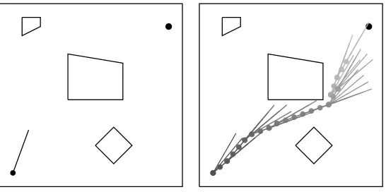
Each task consists of a square workspace that contains a rod, some obstacles, and a target. The agent is required to maneuver the rod so that its tip touches the target (by moving its base coordinate or its angle of orientation) while avoiding obstacles. An example 20x20 unit task and solution path are shown in Figure 1.
Figure 1: A 20x20 rod positioning task and one possible solution path.
Following Moore and Atkeson (1993), we discretize the state space into unit x and y coordi-nates and 10◦ angle increments. Thus, each state in the problem-space can be described by two coordinates and one angle, and the actions available to the agent are movement of one unit in either direction along the rod’s axis, or a 10orotation in either direction. If a movement causes the rod to collide with an obstacle, it results in no change in state, so the portions of the state space where any part of the rod would be interior to an obstacle are not reachable. The agent receives a reward of−1 for each action, and a reward of 1000 when reaching the goal (whereupon the current episode ends). We augment the task environment with five beacons, each of which emits a signal that drops off with the square of the Euclidean distance from a strength of 1 at the beacon to 0 at a distance of 60 units. The tip of the rod has a sensor array that can detect the values of each of these signals separately at the adjacent state in each action direction. Since these beacons are present in every task, the sensor readings are an agent-space and we include an element in the agent that learns L and uses it to predict reward for each adjacent state given the five signal levels present there.
The usefulness of L as a reward predictor will depend on the relationship between beacon place-ment and reward across a sequence of individual rod positioning tasks. Thus we can consider the beacons as simple abstract signals present in the environment, and by manipulating their placement (and therefore their relationship to reward) across the sequence of tasks, we can experimentally evaluate the usefulness of various forms of L.
4.3.1 EXPERIMENTALSTRUCTURE
In each experiment, the agent is exposed to a sequence of training experiences, during which it is allowed to update L. After each training experience, it is evaluated in a large test case, during which it is not allowed to update L.
present at it, before it is tested on the much larger test task. All state value tables are cleared between training episodes.
Each agent performed reinforcement learning using Sarsa(λ)(λ = 0.9,α = 0.1,γ = 0.99,
ε = 0.01) in problem-space and used training tasks that were either 10x10 (where it was given 100 episodes to converge in each training task), or 15x15 (when it was given 150 episodes to converge), and tested in a 40x40 task.3 L was a linear estimator of reward, using either the five beacon signal
levels and a constant as features (requiring 6 parameters, and referred to as the linear model) or using those with five additional features for the square of each beacon value (requiring 11 parameters, referred to as the quadratic model). All parameters were initialized to 0, and learning for L was accomplished using gradient descent with α=0.001. We used two experiments with different beacon placement schemes.
4.3.2 FOLLOWING AHOMINGBEACON
In the first experiment, we always placed the first beacon at the target location, and randomly dis-tributed the remainder throughout the workspace. Thus a high signal level from the first beacon predicts high reward, and the others should be ignored. This is a very informative indication of reward that should be easy to learn, and can be well approximated even with a linear L. Figure 2 shows the 40x40 test task used to evaluate the performance of each agent, and four sample 10x10 training tasks.
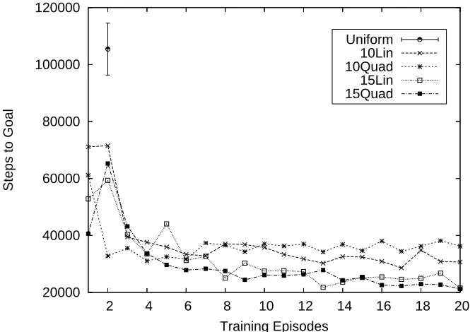
Figure 3(a) shows the number of steps (averaged over 50 runs) required to first reach the goal in the test task, against the number of training tasks completed by the agent for the four types of learned shaping elements (linear and quadratic L, and either 10x10 or 15x15 training tasks). It also shows the average number of steps required by an agent with a uniform initial value of 0 (agents with a uniform initial value of 500 performed similarly while first finding the goal). Note that there is just a single data point for the uniform initial value agents (in the upper left corner) because their performance does not vary with the number of training experiences.
Figure 3(a) shows that training significantly lowers the number of steps required to initially find the goal in the test task in all cases, reducing it after one training experience from over 100,000 steps to at most just over 70,000, and by six episodes to between 20,000 and 40,000 steps. This difference is statistically significant (by a t-test, p<0.01) for all combinations of L and training task sizes, even after just a single training experience. Figure 3(a) also shows that the complexity of L does not appear to make a significant difference to the long-term benefit of training (probably because of the simplicity of the reward indicator), but training task size does. The difference between the number of steps required to first find the goal for 10x10 and 15x15 training task sizes is statistically significant (p<0.01) after 20 training experiences for both linear and quadratic forms of L, although this difference is clearer for the quadratic form, where it is significant after 6 training experiences.
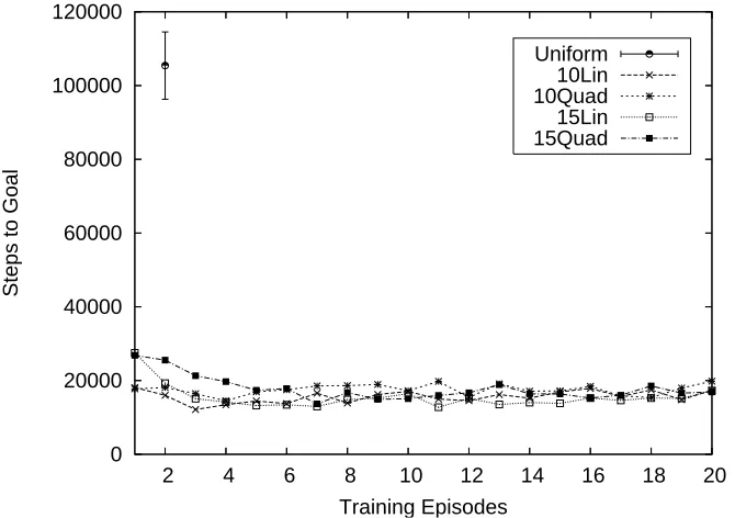
Figure 3(b) shows the number of steps (averaged over 50 runs) required to reach the goal as the agents repeat episodes in the test task, after completing 20 training experiences (note that L is never updated in the test task), compared to the number of steps required by agents with value tables uniformly initialized to 0 and 500. This illustrates the difference in overall learning performance on a single new task between agents that have had many training experiences and agents that have
a b
Figure 2: The homing experiment 40x40 test task (a) and four sample 10x10 training tasks (b). Beacon locations are shown as crosses, and the goal is shown as a large dot. Note that the first beacon is on the target in each task. The optimal solution for the test task requires 69 steps.
not. Figure 3(b) shows that the learned shaping function significantly improves performance during the first few episodes of learning, as expected. It also shows that the number of episodes required for convergence is roughly the same as that of an agent using a uniformly optimistic value table initialization of 500, and slightly longer than that of an agent using a uniformly pessimistic value table initialization of 0. This suggests that once a solution is found the agent must “unlearn” some of its overly optimistic estimates to achieve convergence. Note that a uniform initial value of 0 works well here because it discourages extended exploration, which is unnecessary in this domain.
4.3.3 FINDING THECENTER OF A BEACONTRIANGLE
In the second experiment, we arranged the first three beacons in a triangle at the edges of the task workspace, so that the first beacon lay to the left of the target, the second directly above it, and the third to its right. The remaining two were randomly distributed throughout the workspace. This provides a more informative signal, but results in a shaping function that is harder to learn. Figure 4 shows the 10x10 sample training tasks given in Figure 2 after modification for the triangle experiment. The test task was similarly modified.
20000 40000 60000 80000 100000 120000
2 4 6 8 10 12 14 16 18 20
Steps to Goal
Training Episodes
Uniform 10Lin 10Quad 15Lin 15Quad
(a) The average number of steps required to first reach the goal in the homing test task, for agents that have completed varying numbers of training task episodes.
0 20 40 60 80 100 120 140 160 180 0
1 2 3 4 5 6 7 8 9 10 11x 10
4
Episodes in the Test Task
Steps to Goal
Uni0 Uni500 10Lin 10Quad 15Lin 15Quad
(b) Steps to reward against episodes in the homing test task for agents that have completed 20 training tasks.
Figure 4: Sample 10x10 training tasks for the triangle experiment. The three beacons surrounding the goal in a triangle are shown in gray.
5(a) also shows that there is no significant difference between forms of L and size of training task. This suggests that extra information in the agent-space more than makes up for a shaping function being difficult to accurately represent—in all cases the performance of agents learning using the triangle beacon arrangement is better than that of those learning using the homing beacon arrange-ment. Figure 5(b) shows again that the initial few episodes of repeated learning in the test task are much faster, and again that the total number of episodes required to converge lies somewhere between the number required by an agent initializing its value table pessimistically to 0 and one initializing it optimistically to 500.
4.3.4 SENSITIVITYANALYSIS
So far, we have used shared features that are accurate in the sense that they provide a signal that is uncorrupted by noise and that has exactly the same semantics across tasks. In this section, we empirically examine how sensitive a learned shaping reward might be to the presence of noise, both in the features and in their role across tasks.
To do so, we repeat the above experiments (using training tasks of size 15, and a quadratic approximator) but with only a single beacon whose position is given by the following formula:
b= (1−η)g+ηr,
where g is the coordinate vector of the target,η∈[0,1]is a noise parameter, and r is a co-ordinate vector generated uniformly at random. Thus, whenη=0 we have no noise and the beacon is always placed directly over the goal; when η=1, the beacon is placed randomly in the environment. Varyingη between 0 and 1 allows us to manipulate the amount of noise present in the beacon’s placement, and hence in the shared feature used to learn a portable shaping function. We consider two scenarios.
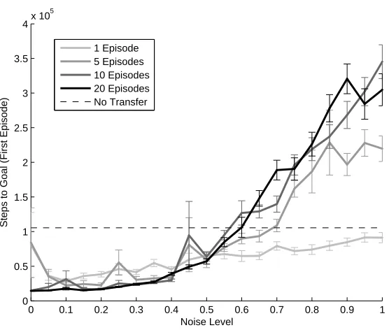
In the first scenario, the sameηvalue is used to place the beacon in both the training and the test problem. This corresponds to a signal that is perturbed by noise, but whose semantics remain the same in both source and target tasks. This measures how sensitive learned shaping rewards are to feature noise, and so we call this the noisy-signal task. The results are shown in Figure 6(a) and 6(b).
0 20000 40000 60000 80000 100000 120000
2 4 6 8 10 12 14 16 18 20
Steps to Goal
Training Episodes
Uniform 10Lin 10Quad 15Lin 15Quad
(a) The average number of steps required to first reach the goal in the triangle test task, for agents that have completed varying number of training task episodes.
0 20 40 60 80 100 120 140 160
0 1 2 3 4 5 6 7 8 9 10 11x 10
4
Episodes in the Test Task
Steps to Goal
Uni0 Uni500 10Lin 10Quad 15Lin 15Quad
(b) Steps to reward against episodes in the triangle test task for agents that have completed 20 training tasks.
0 0.1 0.2 0.3 0.4 0.5 0.6 0.7 0.8 0.9 1 0
0.5 1 1.5 2
2.5x 10
5
Noise Level
Steps to Goal (First Episode)
1 Episode 5 Episodes 10 Episodes 20 Episodes No Transfer
(a) The average number of steps required to first reach the test task goal given a predictor learned using a noisy signal.
0 20 40 60 80 100 120 140 160
0 0.5 1 1.5 2
x 105
Episodes in the Test Task
Steps to Goal
Noise=0.4 Noise=0.6 Noise=0.8 Noise=1.0 Uniform 0 Uniform 500
(b) Steps to reward against episodes in the test task for agents that have completed 20 training task episodes using a noisy signal.
scratch that drops with increased noise but still does better untilη>0.6, when the feature has more noise than signal.
Higher levels of noise more severely affects agents that have seen higher numbers of training problems, until a performance floor is reached between 5 and 10 training problems. This reflects the training procedure used to learn L, whereby each training problem results in a small adjustment of L’s parameters and those adjustments accumulate over several training episodes.
Similarly, Figure 6(b) shows learning curves in the test problem for agents that have experienced 20 test problems, with varying amounts of noise. We see that, although these agents often do worse than learning from scratch in the first episode, they subsequently do better whenη<1, and again converge at roughly the same rate as agents that use an optimistic initial value function.
In the second scenario, η is zero in the training problems, but non-zero in the test problem. This corresponds to a feature which has slightly different semantics in the source and target tasks, and thus measures how learning is affected by an imperfect or approximate choice of agent space features. We call this the noisy-semantics task.
Results for the noisy-semantics task are given in Figures 7(a) and 7(b). These two graphs show that transfer achieves a performance benefit whenη<0.5—when there is at least as much signal as noise—and the more training problems the agent has solved, the worse its performance will be whenη=1. However, the possible performance penalty for highηis more severe—an agent using a learned shaping function that rewards it for following a beacon signal may take nearly four times as long to first solve the test problem when that feature becomes random (atη=1). Again, however, whenη<1 the agents recover after their first episode to outperform agents that learn from scratch within the first few episodes.
4.3.5 SUMMARY
The first two experiments above show that an agent able to learn its own shaping rewards through training can use even a few training experiences to significantly improve its initial policy in a novel task. They also show that such training results in agents with convergence characteristics similar to that of agents using uniformly optimistic initial value functions. Thus, an agent that learns its own shaping rewards can improve its initial speed at solving a task when compared to an agent that cannot, but it will not converge to an approximately optimal policy in less time (as measured in episodes).
The results also seem to suggest that a better training environment is helpful but that its useful-ness decreases as the signal predicting reward becomes more informative, and that increasing the complexity of the shaping function estimator does not appear to significantly improve the agent’s performance. Although this is a very simple domain, this suggests that given a rich signal from which to predict reward, even a weak estimator of reward can greatly improve performance.
0 0.1 0.2 0.3 0.4 0.5 0.6 0.7 0.8 0.9 1 0
0.5 1 1.5 2 2.5 3 3.5
4x 10
5
Noise Level
Steps to Goal (First Episode)
1 Episode 5 Episodes 10 Episodes 20 Episodes No Transfer
(a) The average number of steps required to first reach the test task goal given a predictor learned using features with imperfectly preserved semantics.
0 20 40 60 80 100 120 140 160
0 0.5 1 1.5 2 2.5 3 3.5
x 105
Episodes in the Test Task
Steps to Goal
Noise=0.4 Noise=0.6 Noise=0.8 Noise=1.0 Uniform 0 Uniform 500
(b) Steps to reward against episodes in the test task for agents that have completed 20 training task episodes using features with imperfectly preserved semantics.
4.4 Keepaway
In this section we evaluate knowledge transfer using common features in Keepaway (Stone et al., 2005), a robot soccer domain implemented in the RoboCup soccer simulator. Keepaway is a chal-lenging domain for reinforcement learning because it is multi-agent and has a high-dimensional continuous state space. We use Keepaway to illustrate the use of learned shaping rewards on a stan-dard but challenging benchmark that has been used in other transfer studies (Taylor et al., 2007).
Keepaway has a square field of a given size, which contains players and a ball. Players are divided into two groups: keepers, who are originally in possession of the ball and try to stay in control of it, and takers, who attempt to capture the ball from the keepers. This arrangement is depicted in Figure 8.
Figure 8: The Keepaway Task. The keepers (white circles) must keep possession of the ball and not allow the takers (gray octagons) to take it away. This diagram depicts 3v2 Keepaway, where there are 3 keepers and 2 takers.
Each episode begins with the takers in one corner of the field and the keepers randomly dis-tributed. The episode ends when the ball goes out of bounds, or when a taker ends up in possession of the ball (i.e., within a small distance of the ball for a specified period of time). The goal of the keepers is then to maximize the duration of the episode. At each time step, the objective of learning is to modify the behavior of the keeper currently in possession of the ball. The takers and other keepers act according to simple hand-coded behaviors. Keepers not in possession of the ball try to open a clear shot from the keeper with the ball to themselves and attempt to receive the ball when it is passed to them. Takers either try to block keepers that are not holding the ball, try to take the ball from the keeper in possession, or try to intercept a pass.
Rather than using the primitive actions of the domain, keepers are given a set of predefined options. The options available to the keeper in possession of the ball are HoldBall (remain stationary while keeping the ball positioned away from the takers) and PassBall(k) (pass the ball to the kth other keeper). Since only the keeper in possession of the ball is acting according to the reinforcement learner at any given time, multiple keepers may learn during each episode; each keeper’s learner runs separately.
from K1 (the keeper in possession) to each other player, the minimum angles BAC for each other keeper (where B is the other keeper, A is K1, and C is a taker—this measures how “open” each other keeper is to a pass), the distance from each player to the center, and the minimum distance from each other keeper to a taker. The number of state variables is 4K+2T−3, for K keepers and T takers. We used a field measuring 20x20 units for 3v2 games, and a field measuring 30x30 for 4v3 and 5v4. For a more detailed description of the Keepaway domain we refer the reader to Stone et al. (2005).
4.4.1 EXPERIMENTALSTRUCTURE
In the previous section, we studied transferring portable shaping functions from a varying number of smaller randomly generated source tasks to a fixed larger target task. In Keepaway, instances of the domain are obtained by fixing the number of keepers and the number of takers. Since we cannot obtain experience in more than a few distinct source tasks, in this section we instead study the effect of varying amounts of training time in a source task on performance in a target task.
We thus studied transfer from 3v2 Keepaway to 4v3 and 5v4 Keepway, and from 4v3 to 5v4; these are the most common Keepaway configurations and are the same configurations studied by Taylor and Stone (2005). In all three cases we used the state variables from 5v4 as an agent-space. When a state variable is not defined (e.g., the distance to the 4th keeper in 3v2 Keepaway), we set distances and angles to keepers to 0, and distances and angles to takers to their maximum value, which effectively simulates their being present but not meaningfully involved in the current state. We employed linear function approximation with Sarsa (Sutton and Barto, 1998) using 32 radial basis functions per state variable, tiling each variable independently of the others, following and using the same parameters as Stone et al. (2005).
We performed 20 separate runs for each condition. We first ran 20 baseline runs for 3v2, 4v3, and 5v4 Keepaway, saving weights for the common space for each 3v2 and 4v3 run at 50, 250, 500, 1000, 2000, and 5000 episodes. Then for each set of common space weights from a given number of episodes, we ran 20 transfer runs. For example, for the 3v2 to 5v4 transfer with 250-episode weights, we ran 20 5v4 transfer runs, each of which used one of the 20 saved 250-episode 3v2 weights.
Because of Keepaway’s high variance, and in order to provide results loosely comparable with Taylor and Stone (2005), we evaluated the performance of transfer in Keepaway by measuring the average time required to reach some benchmark performance. We selected a benchmark time for each setting (3v2, 4v3 or 5v4) which the baseline learner could consistently reach by about 5000 episodes. This benchmark time T is considered reached at episode n when the average of the times from n−500 to n+500 is at least T ; this window averaging compensates Keepaway’s high performance variance. The benchmark times for each domain were, in order, 12.5 seconds, 9.5 seconds, and 8.5 seconds.
4.4.2 RESULTS
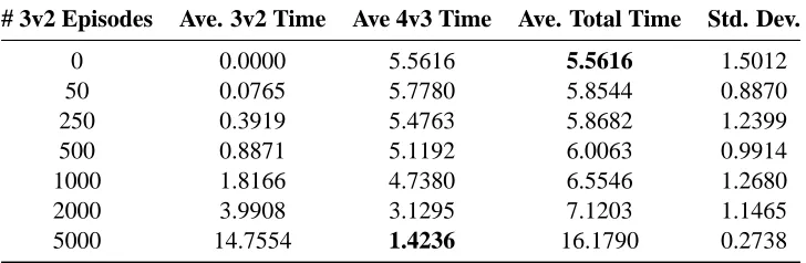
in the target task with experience in the source task—by examining the third column (average 4v3 time), and strong transfer—where the sum of the time spent in both source and target tasks is lower than that taken when learning the target task in isolation—by examining the fourth column (average total time).
The results show that training in 3v2 decreases the amount of time required to reach the bench-mark in 4v3, which shows that transfer is successful in this case and weak transfer is achieved. However, the total (source and target) time to benchmark never decreases with experience in the source task, so strong transfer is not achieved.
# 3v2 Episodes Ave. 3v2 Time Ave 4v3 Time Ave. Total Time Std. Dev.
0 0.0000 5.5616 5.5616 1.5012
50 0.0765 5.7780 5.8544 0.8870
250 0.3919 5.4763 5.8682 1.2399
500 0.8871 5.1192 6.0063 0.9914
1000 1.8166 4.7380 6.5546 1.2680
2000 3.9908 3.1295 7.1203 1.1465
5000 14.7554 1.4236 16.1790 0.2738
Table 1: Results of transfer from 3v2 Keepaway to 4v3 Keepaway.
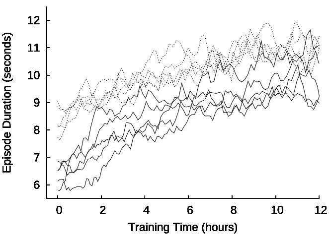
Figure 9 shows sample learning curves for agents learning from scratch and agents using trans-ferred knowledge from 5000 episodes of 3v2 Keepaway, demonstrating that agents that transfer knowledge start with better policies and learn faster.
Table 2 shows the results of transfer from 3v2 Keepaway (Table 1(a)) and 4v3 Keepaway (Table 1(b)) to 5v4 Keepaway. As before, in both cases more training on the easier task results in better performance in 5v4 Keepaway, demonstrating that weak transfer is achieved. However, the least total time (including training time on the source task) is obtained using a moderate amount of source task training, and so when transferring to 5v4 we achieve strong transfer.
Finally, Table 3 shows the results of transfer for shaping functions learned on both 3v2 and 4v3 Keepaway, applied to 5v4 Keepaway. Again, more training time obtains better results although over-training appears to be harmful.
These results show that knowledge transfer through agent-space can achieve effective transfer in a challenging problem and can do so in multiple problems through the same set of common features.
4.5 Discussion
The results presented above suggest that agents that employ reinforcement learning methods can be augmented to use their experience to learn their own shaping rewards. This could result in agents that are more flexible than those with pre-engineered shaping functions. It also creates the possibility of training such agents on easy tasks as a way of equipping them with knowledge that will make harder tasks tractable, and is thus an instance of an autonomous developmental learning system (Weng et al., 2000).
6 7 8 9 10 11 12
0 2 4 6 8 10 12
Episode Duration (seconds)
Training Time (hours) 6 7 8 9 10 11 12
0 2 4 6 8 10 12
Episode Duration (seconds)
Training Time (hours) 6 7 8 9 10 11 12
0 2 4 6 8 10 12
Episode Duration (seconds)
Training Time (hours) 6 7 8 9 10 11 12
0 2 4 6 8 10 12
Episode Duration (seconds)
Training Time (hours) 6 7 8 9 10 11 12
0 2 4 6 8 10 12
Episode Duration (seconds)
Training Time (hours) 6 7 8 9 10 11 12
0 2 4 6 8 10 12
Episode Duration (seconds)
Training Time (hours) 6 7 8 9 10 11 12
0 2 4 6 8 10 12
Episode Duration (seconds)
Training Time (hours) 6 7 8 9 10 11 12
0 2 4 6 8 10 12
Episode Duration (seconds)
Training Time (hours) 6 7 8 9 10 11 12
0 2 4 6 8 10 12
Episode Duration (seconds)
Training Time (hours) 6 7 8 9 10 11 12
0 2 4 6 8 10 12
Episode Duration (seconds)
Training Time (hours)
Figure 9: Sample learning curves for 4v3 Keepaway given no transfer (solid lines) or having expe-rienced 5000 episodes of experience in 3v2 (dashed lines).
potential concern is the possibility that a maliciously chosen or unfortunate set of training tasks could result in an agent that performs worse than one with no training. Fortunately, such agents will still eventually be able to learn the correct value function (Ng et al., 1999).
All of the experiments reported in this paper use model-free learning algorithms. Given that an agent facing a sequence of tasks receives many example transitions between pairs of space descriptors, it may prove efficient to instead learn an approximate transition model in agent-space and then use that model to obtain a shaping function via planning. However, learning a good transition model in such a scenario may prove difficult because the agent-space features are not Markov.
In standard classical search algorithms such as A∗, a heuristic imposes an order in which nodes are considered during the search process. In reinforcement learning the state space is searched by the agent itself, but its initial value function (either directly or via a shaping function) acts to order the selection of unvisited nodes by the agent. Therefore, we argue that reinforcement learning agents using non-uniform initial value functions are using something very similar to a heuristic, and those that are able to learn their own portable shaping functions are in effect able to learn their own heuristics.
5. Skill Transfer
(a) Transfer results from 3v2 to 5v4 Keepaway.
# 3v2 Episodes Ave. 3v2 Time Ave 5v4 Time Ave. Total Time Std. Dev.
0 0.0000 7.4931 7.4931 1.5229
50 0.0765 6.3963 6.4728 1.0036
250 0.3919 5.6675 6.0594 0.7657
500 0.8870 5.9012 6.7882 1.1754
1000 1.8166 3.9817 5.7983 1.2522
2000 3.9908 3.9678 7.9586 1.8367
5000 14.7554 3.9241 18.6795 1.3228
(b) Transfer results from 4v3 to 5v4 Keepaway.
# 4v3 Episodes Ave. 4v3 Time Ave 5v4 Time Ave. Total Time Std. Dev.
0 0.0000 7.4931 7.4930 1.5229
50 0.0856 6.6268 6.7125 1.2162
250 0.4366 6.1323 6.5689 1.1198
500 0.8951 6.3227 7.2177 1.0084
1000 1.8671 6.0406 7.9077 1.0766
2000 4.0224 5.0520 9.0744 0.9760
5000 11.9047 3.218 15.1222 0.6966
Table 2: Results of transfer to 5v4 Keepaway.
# 3v2 Episodes # 4v3 Episodes Ave 5v4 Time Ave. Total Time Std. Dev.
500 500 6.1716 8.0703 1.1421
500 1000 5.6139 8.6229 0.9597
1000 500 4.5395 7.3922 0.6689
1000 1000 4.8648 8.8448 0.9517
Table 3: Results of transfer from both 3v2 Keepaway and 4v3 Keepaway to 5v4 Keepaway.
performance. We can apply the same framework to effect skill transfer by creating portable option policies. Most option learning methods work within the same state space as the problem the agent is solving at the time. Although this can lead to faster learning on later tasks in the same state space, learned options would be more useful if they could be reused in later tasks that are related but have distinct state spaces.
5.1 Options in Agent-Space
Following section 4.2, we consider an agent solving n problems M1, ...,Mnwith state spaces S1, ...,Sn,
and action space A. Once again, we associate a four-tupleσij with the ith state in Mj:
σj i =hs
j i,d
j i,r
j i,v
j ii,
where sij is the usual problem-space state descriptor (sufficient to distinguish this state from the others in Sj), dij is the agent-space descriptor, r
j
i is the reward obtained at the state and v j i is the
state’s value (expected total reward for action starting from the state).
The agent is also either given, or learns, a set of higher-level options to reduce the time required to solve the task. Options defined using sij are not portable between tasks because the form and meaning of sij (as a problem-space descriptor) may change from one task to another. However, the form and meaning of dij (as an agent-space descriptor) does not. Therefore we define agent-space option components as:
πo: (dij,a) 7→[0,1],
Io: dij 7→ {0,1},
βo: dij 7→[0,1].
Although the agent will be learning task and option policies in different spaces, both types of poli-cies can be updated simultaneously as the agent receives both agent-space and problem-space de-scriptors at each state.
To support learning a portable shaping function, an agent space should contain some features that are correlated to return across tasks. To support successful skill policy learning, an agent space needs more: it must be suitable for directly learning control policies.
If that is the case, then why not perform task learning (in addition to option learning) in agent-space? There are two primary reasons why we might prefer to perform task learning in problem-space, even when given an agent-space suitable for control learning. The first is that agent-space may be very much larger than problem-space, making directly learning the entire task in agent-space inefficient or impractical. The second is that the agent-space may only be sufficient for learning control policies locally, rather than globally. In the next two sections we demonstrate portable skill learning on domains with each characteristic in turn.
5.2 The Lightworld Domain
The lightworld domain is a parameterizable class of discrete domains which share an agent-space that is much larger than any individual problem-space. In this section, we empirically examine whether learning portable skills can improve performance in such a domain.
In order to specify an individual lightworld instance, we must specify the number of rooms, x and y sizes for each room, and the location of the room entrance, key (or lack therefore), lock and door in each. Thus, we may generate new lightworld instances by generating random values for each of these parameters.
We equip the agent with twelve light sensors, grouped into threes on each of its sides. The first sensor in each triplet detects red light, the second green and the third blue. Each sensor responds to light sources on its side of the agent, ranging from a reading of 1 when it is on top of the light source, to 0 when it is 20 squares away. Open doors emit a red light, keys on the floor (but not those held by the agent) emit a green light, and locks emit a blue light. Figure 10 shows an example.
Figure 10: A small example lightworld.
Five pieces of data form a problem-space descriptor for any lightworld instance: the current room number, the x and y coordinates of the agent in that room, whether or not the agent has the key, and whether or not the door is open. We use the light sensor readings as an agent-space because their semantics are consistent across lightworld instances. In this case the agent-space (with 12 continuous variables) has much higher dimension than any individual problem-space, and it is impractical to perform task learning in it directly, even though the problem might in principle be solvable that way.
5.2.1 TYPES OFAGENT
We used five types of reinforcement learning agents: agents without options, agents with problem-space options, agents with perfect problem-problem-space options, agents with agent-problem-space options, and agents with both option types.
The agents without options used Sarsa(λ) with ε-greedy action selection (α=0.1, γ=0.99,
λ=0.9,ε=0.01) to learn a solution policy in problem-space, with each state-action pair assigned an initial value of 500.
off-policy trace-based tree-backup updates (Precup et al., 2000) for intra-option learning. We used an option termination reward of 1 for successful completion, and a discount factor of 0.99 per action. Options could be executed only in the room in which they were defined and only in states where their value function exceeded a minimum threshold (0.0001). Because these options were learned in problem-space, they were useful but needed to be relearned for each individual lightworld.
Agents with perfect problem-space options were given options with pre-learned policies for each salient event, though they still performed option updates and were otherwise identical to the standard agent with options. They represent the ideal case of agents with that can perform perfect transfer, arriving in a new task with fully learned options.
Agents with agent-space options still learned their solution policies in problem-space but learned their option policies in agent-space. Each agent employed three options: one for picking up a key, one for going through an open door and one for unlocking a door, with each one’s policy a function of the twelve light sensors. Since the sensor outputs are continuous we employed linear function approximation for each option’s value function, performing updates using gradient descent (α=0.01) and off-policy trace-based tree-backup updates. We used an option termination reward of 1, a step penalty of 0.05 and a discount factor of 0.99. An option could be taken at a particular state when its value function there exceeded a minimum threshold of 0.1. Because these options were learned in agent-space, they could be transferred between lightworld instances.
Finally, agents with both types of options were included to represent agents that learn both general portable and specific non-portable skills simultaneously.
Note that all agents used discrete problem-space value functions to solve the underlying task instance, because their agent-space descriptors are only Markov in lightworlds with a single room, which were not present in our experiments.
5.2.2 EXPERIMENTALSTRUCTURE
We generated 100 random lightworlds, each consisting of 2-5 rooms with width and height of be-tween 5 and 15 cells. A door and lock were randomly placed on each room boundary, and 13 of rooms included a randomly placed key. This resulted in state space with between 600 and approxi-mately 20,000 state-action pairs (4,900 on average). We evaluated each problem-space option agent type on 1000 lightworlds (10 samples of each generated lightworld).
To evaluate the performance of agent-space options as the agents gained more experience, we similarly obtained 1000 lightworld samples and test tasks, but for each test task we ran the agents once without training and then with between 1 and 10 training experiences. Each training experience for a test lightworld task consisted of 100 episodes in a training lightworld randomly selected from the remaining 99. Although the agents updated their options during evaluation in the test lightworld, these updates were discarded before the next training experience so the agent-space options never received prior training in the test lightworld.
5.2.3 RESULTS
better performance than an agent using problem-space options alone, until by 5 experiences its learning curve is similar to that of an agent with perfect problem-space options (compare the learn-ing curves in Figure 11(b) with the bottom-most learnlearn-ing curve of Figure 11(a)), even though its options are never trained in the same lightworld in which it is tested. The comparison between Figures 11(a) and 11(b) shows that agent-space options can be successfully transferred between lightworld instances.
10 20 30 40 50 60 70
0 1000 2000 3000 4000 5000 6000 7000 Episodes Actions Perfect Options Learned Options No Options
(a) Learning curves for agents with problem-space op-tions.
10 20 30 40 50 60 70
0 1000 2000 3000 4000 5000 6000 7000 Episodes Actions 0 experiences 1 experience 2 experiences 5 experiences 10 experiences
(b) Learning curves for agents with agent-space options, with varying numbers of training experiences.
10 20 30 40 50 60 70
0 1000 2000 3000 4000 5000 6000 7000 Episodes Actions 0 experiences 1 experience 2 experiences 5 experiences 10 experiences
(c) Learning curves for agents with agent-space and problem-space options, with varying numbers of training experiences.
NO LO PO 0 1 2 3 4 5 6 7 8 9 10 0 2 4 6 8 10 12 14x 10
5
(d) Total steps over 70 episodes for agents with no options (NO), learned problem-space options (LO), perfect options (PO), agent-space options with 0-10 training experiences (dark bars), and both option types with 0-10 training expe-riences (light bars).
Figure 11: Results for the Lightworld Domain.
Figure 11(c) shows average learning curves for agents employing both types of options.4 The first time such agents encounter a lightworld, they perform as well as agents using problem-space
options (compare with the second highest curve in Figure 11(a)), and thereafter rapidly improve their performance (performing better than agents using only agent-space options) and again by 5 experiences performed nearly as well as agents with perfect options. This improvement can be explained by two factors. First, the agent-space is much larger than any individual problem-space, so problem-space options are easier to learn from scratch than agent-space options. This explains why agents using only agent-space options and no training experiences perform more like agents without options than like agents with problem-space options. Second, options learned in our problem-space can represent exact solutions to specific subgoals, whereas options learned in our agent-space are general and must be approximated, and are therefore likely to be slightly less efficient for any specific subgoal. This explains why agents using both types of options perform better in the long run than agents using only agent-space options.
Figure 11(d) shows the mean total number of steps required over 70 episodes for agents using no options, problem-space options, perfect options, agent-space options, and both option types. Experience in training environments rapidly drops the number of total steps required to nearly as low as the number required for an agent with perfect options. It also clearly shows that agents using both types of options do consistently better than those using agent-space options alone. We note that the error bars in Figure 11(d) are small and decrease with experience, indicating consistent transfer.
In summary, these results show that learning using portable options can greatly improve per-formance over learning using problem-specific options. Given enough experience, learned portable options can perform similarly to perfect pre-learned problem-specific options, even when the agent-space is much harder to learn in than any individual problem-agent-space. However, the best learning strategy is to learn using both problem-specific options and portable options.
5.3 The Conveyor Belt Domain
In the previous section we showed that an agent can use experience in related tasks to learn portable options, and that those options can improve performance in later tasks, when the agent has a dimensional agent-space. In this section we consider a task where the agent-space is not high-dimensional, but is only sufficient for local control.
In the conveyor belt domain, a conveyor belt system must move a set of objects from a row of feeders to a row of bins. There are two types of objects (triangles and squares), and each bin starts with a capacity for each type. The objects are issued one at a time from a feeder and must be directed to a bin. Dropping an object into a bin with a positive capacity for its type decrements that capacity.
Each feeder is directly connected to its opposing bin through a conveyor belt, which is connected to the belts above and below it at a pair of fixed points along its length. The system may either run the conveyor belt (which moves the current object one step along the belt) or try to move it up or down (which only moves the object if it is at a connection point). Each action results in a reward of
−1, except where it causes an object to be dropped into a bin with spare capacity, in which case it results in a reward of 100. Dropping an object into a bin with zero capacity for that type results in the standard reward of−1.
To specify an instance of the conveyor belt domain, we must specify the number of objects present, belts present, bin capacities, belt length, and where each adjacent pair of belts are con-nected. A small example conveyor belt system is shown in Figure 12.
1
2
3
Figure 12: A small example conveyor belt problem.
Each system has a camera that tracks the current object and returns values indicating the distance (up to 15 units) to the bin and each connector along the current belt. Because the space generated by the camera is present in every conveyor-belt problem and retains the same semantics, it is an agent-space, and because it is discrete and relatively small (13,500 states), we can learn policies in it without function approximation. However, because it is non-Markov (due to its limited range and inability to distinguish between belts), it cannot be used as a problem-space.
A problem-space descriptor for a conveyor belt instance consists of three numbers: the current object number, the belt it is on, and how far along that belt it lies (technically we should include the current capacity of each bin, but we can omit this and still obtain good policies). We generated 100 random instances with 30 objects and 20-30 belts (each of length 30-50) with randomly-selected interconnections, resulting in problem-spaces of 18,000-45,000 states.
We ran experiments where the agents learned three options: one to move the current object to the bin at the end of the belt it is currently on, one for moving it to the belt above it, and one for moving it to the belt below it. We used the same agent types and experimental structure as before, except that the agent-space options did not use function approximation.
5.3.1 RESULTS
Figures 13(a), 13(b) and 13(c) show learning curves for agents employing no options, problem-space options and perfect options; agents employing agent-problem-space options; and agents employing both types of options, respectively.
0 10 20 30 40 50 60 70 −5000 −4000 −3000 −2000 −1000 0 1000 Episodes Reward Learned Options Perfect Options No Options
(a) Learning curves for agents with problem-space op-tions.
0 10 20 30 40 50 60 70 −5000 −4000 −3000 −2000 −1000 0 1000 Episodes Reward 0 experiences 1 experience 3 experiences 5 experiences 8 experiences 10 experiences
(b) Learning curves for agents with agent-space options, with varying numbers of training experiences.
0 10 20 30 40 50 60 70
−5000 −4000 −3000 −2000 −1000 0 1000 Episodes Reward 0 experiences 1 experience 3 experiences 5 experiences 8 experiences 10 experiences
(c) Learning curves for agents with both types of options, with varying numbers of training experiences.
NO LO PO 0 1 2 3 4 5 6 7 8 9 10
−8 −6 −4 −2 0 2 4
x 104
(d) Total reward over 70 episodes for agents with no op-tions (NO), learned problem-space opop-tions (LO), perfect options (PO), agent-space options with 0-10 training expe-riences (dark bars), and both option types with 0-10 train-ing experiences (light bars).
Figure 13: Results for the Conveyor Belt Domain.
Figure 13(c) shows that agents with both option types do not experience this initial dip relative to agents with no prior experience and outperform problem-space options immediately, most likely because the agent-space options are able to generalise across belts. Figure 13(d) shows the mean total reward for each type of agent. Agents using agent-space options eventually outperform agents using problem-space options only, even though the agent-space options have a much more limited range; agents using both types of options consistently outperform agents with either option type and eventually approach the performance of agents using pre-learned problem-space options.
perfor-mance of perfect pre-learned problem-specific options. Once again, the best approach is to learn using both problem-specific and agent-space options simultaneously.
5.4 Summary
Our results show that options learned in agent-space can be successfully transferred between related tasks, and that this significantly improves performance in sequences of tasks where the agent space cannot be used for learning directly. Our results suggest that when the agent space is large but can support global policies, experience in related tasks can eventually result in options that perform as well as perfect problem-specific options. When the agent space is only locally Markov, learned portable options will improve performance but are unlikely to reach the performance of perfect problem-specific options due to their limited range.
We expect that, in general, learning an option in agent-space will often actually be harder than solving an individual problem-space instance, as was the case in our experiments. In such situations, learning both problem-specific and agent space options simultaneously will likely obtain better performance than either individually. Since intra-option learning methods allow for the update of several options from the same experiences, it may be better in general to simultaneously learn both general portable skills and specific, exact but non-portable skills, and allow them to bootstrap each other.
6. Related Work
Although the majority of research in transfer assumes that the source and target problems have the same state space, some existing research does not make that assumption.
Wilson et al. (2007) consider the case where an agent faces a sequence of environments, each generated by one of a set of environment classes. Each environment class is modeled as a distri-bution of values of some observed signal given a feature vector, and since the number of classes is unknown, the agent must learn an infinite mixture model of classes. When faced with a new environment, the agent determines which of its existing models it best matches or whether it instead corresponds to a novel class. A model-based planning algorithm is then used to solve the new task. This work explicitly considers environment sequences that do not have the same state space, and thus defines the distributions of each environment class over the output of a function f that generates a feature vector for each state in each environment. Since that feature vector retains its semantics across all of the tasks, it is exactly an agent-space descriptor as defined here. Thus, this work can be seen as using agent-space to learn a set of environment models.
Banerjee and Stone (2007) consider transfer learning for the case of General Game Playing, where knowledge gained from playing one game (e.g., Tic-Tac-Toe) is exploited to improve perfor-mance in another (e.g., Connect-4). Here, transfer is affected through the game tree: the authors define generic game-tree features that apply across all games and then use their Q-values to initial-ize the values of novel states with matching features when playing a subsequent game. This is a very similar mechanism to a portable shaping function, including the use of features—in this case derived from the game tree—that are common across all tasks.