Characterization and Greedy Learning of Interventional Markov
Equivalence Classes of Directed Acyclic Graphs
Alain Hauser [email protected]
Peter B ¨uhlmann [email protected]
Seminar f¨ur Statistik ETH Z¨urich
8092 Z¨urich, Switzerland
Editor:Max Chickering
Abstract
The investigation of directed acyclic graphs (DAGs) encoding the same Markov property, that is the same conditional independence relations of multivariate observational distributions, has a long tradition; many algorithms exist for model selection and structure learning in Markov equivalence classes. In this paper, we extend the notion of Markov equivalence of DAGs to the case of interven-tional distributions arising frommultipleintervention experiments. We show that under reasonable assumptions on the intervention experiments, interventional Markov equivalence defines a finer par-titioning of DAGs than observational Markov equivalence and hence improves the identifiability of causal models. We give a graph theoretic criterion for two DAGs being Markov equivalent under interventions and show that each interventional Markov equivalence class can, analogously to the observational case, be uniquely represented by a chain graph calledinterventional essential graph
(also known asCPDAGin the observational case). These are key insights for deriving a general-ization of the Greedy Equivalence Search algorithm aimed at structure learning from interventional data. This new algorithm is evaluated in a simulation study.
Keywords: causal inference, interventions, graphical model, Markov equivalence, greedy equiva-lence search
1. Introduction
Directed acyclic graphs (or DAGs for short) are commonly used to model causal relationships be-tween random variables; in such models, parents of some vertex in the graph are understood as “causes”, and edges have the meaning of “causal influences”. The causal influences between ran-dom variables imply conditional independence relations among them. However, those independence
relations, or the corresponding Markov properties, do not identify the corresponding DAG
com-pletely, but only up to Markov equivalence. To put it simple, the skeleton of an underlying DAG is
completely determined by its Markov property, whereas thedirection of the arrows (which is
cru-cial for causal interpretation) is in general not encoded in the Markov property for the observational distribution.
This paper has two main contributions. The first one is an algorithmically tractable graphical representation of Markov equivalence classes under a given set of interventions (possibly affecting several variables) from which the identifiability of causal models can be read off. This is of general interest for computation and algorithms dealing with structure (DAG) learning from an ensemble of observational and interventional data such as MCMC. The second contribution is a generalization of the Greedy Equivalence Search (GES) algorithm of Chickering (2002b), yielding an algorithm called Greedy Interventional Equivalence Search (GIES) which can be used for regularized maxi-mum likelihood estimation in such an interventional setting.
In Section 2, we establish a criterion for two DAGs being Markov equivalent under a given intervention setting. We then generalize the concept of essential graphs, a graph theoretic represen-tation of Markov equivalence classes, to the interventional case and characterize the properties of those graphs in Section 3. In Section 4, we elaborate a set of algorithmic operations to efficiently traverse the search space of interventional essential graphs and finally present the GIES algorithm. An experimental evaluation thereof is given in Section 5. We postpone all proofs to Appendix B, while Appendix A contains a review on graph theoretic concepts and definitions. An
implementa-tion of the GIES algorithm will be available in the next release of the R package pcalg(Kalisch
et al., 2012); meanwhile, a prerelease version is available upon request from the first author.
1.1 Related Work
The investigation of Markov equivalence classes of directed graphical models has a long tradi-tion, perhaps starting with the criterion for two DAGs being Markov equivalent by Verma and Pearl (1990) and culminating in the graph theoretic characterization of essential graphs (also called
CPDAGs, “completed partially directed acyclic graphs”) representing Markov equivalence classes by Andersson et al. (1997). Several algorithms for estimating essential graphs from observational data exist, such as the PC algorithm (Spirtes et al., 2000) or the Greedy Equivalence Search (GES) algorithm (Meek, 1997; Chickering, 2002b); a more complete overview is given in Brown et al. (2005) and Murphy (2001).
Different approaches to incorporate interventional data for learning causal models have been developed in the past. The Bayesian procedures of Cooper and Yoo (1999) or Eaton and Murphy (2007) address the problem of calculating a posterior (and also a likelihood) of an ensemble of ob-servational and interventional data but do not address questions of identifiability or Markov equiv-alence: allowing different posteriors for Markov equivalent models can be intended in Bayesian methods (and realized by giving the corresponding models different priors). Since the number of
DAGs with pvariables grows super-exponentially with p(Robinson, 1973), the computation of a
address the issue of Markov equivalence therewith. Eberhardt et al. (2005) and Eberhardt (2008) provide algorithms for choosing intervention targets thatcompletelyidentifyallcausal models ofp
variables uniformly, but neither address the question of partial identifiability under a limited number of interventions nor provide an algorithm for learning the causal structure from data. Eberhardt et al. (2010) present an algorithm for learningcycliclinear causal models, but focus on complete identi-fiability; identifiability results for cyclic models only implysufficient, but notnecessary, conditions for the identifiability of acyclic models.
Probably the most advanced result concerning identifiability of causal models under single-variable interventions so far is given in the work of Tian and Pearl (2001). Although they do not provide a characterization of equivalence classes as a whole (as this paper does), they present a necessary and sufficient graph theoretic criterion for two models being indistinguishable under a set of single-variable interventions as well as a learning algorithm based on the detection of changes in marginal distributions.
2. Model
We considerprandom variables(X1, . . . ,Xp) =:Xwhich take values in some product measure space (X,A,µ) = (∏ip=1Xi,Nip=1Ai,Nip=1µi)withXi⊂R∀i. Eachσ-algebraAiis assumed to contain
at least two disjoint sets of positive measure to avoid pathologies, andXis assumed to have a strictly positive joint density w.r.t. the measureµonX. We denote the set of all positive densities onX by
M. For any subset of component indicesA⊂[p]:={1, . . . ,p}, we use the notationXA:=∏a∈AXa, XA:= (Xa)a∈Aand the conventionX/0≡0. Lowercase symbols likexArepresent a value inXA.
The model we are considering is built upon Markov properties with respect to DAGs. By con-vention, all graphs appearing in the paper shall have the vertex set[p], representing the prandom variablesX1, . . . ,Xp. Our notation and definitions related to graphs are summarized in Appendix
A.1.
2.1 Causal Calculus: A Short Review
We start by summarizing important facts and fixing our notation concerning Markov properties and intervention calculus.
Definition 1 (Markov property; Lauritzen, 1996) Let D be a DAG. Then we say that a proba-bility density f ∈ M obeys the Markov property ofD if f(x) =∏ip=1f(xi|xpaD(i)). The set of all
positive densities obeying the Markov property of D is denoted byM(D).
Definition 1 is the most straightforward translation of independence relations induced from structural equations, the historical origin of directed graphical models (Wright, 1921). Related notions like local and global Markov properties exist and are equivalent to the factorization property of Definition 1 for positive densities (Lauritzen, 1996).
Definition 2 (Markov equivalence; Andersson et al., 1997) Let D1and D2be two DAGs. D1and
D2are calledMarkov equivalent(notation: D1∼D2) ifM(D1) =M(D2).
Theorem 3 (Verma and Pearl, 1990) Two DAGs D1and D2are Markov-equivalent if and only if
Directed graphical models allow for an obvious causal interpretation. For a density f that obeys
the Markov properties of some DAGD, we can think of a random variableXabeing thedirect cause
of another variableXbifais a parent ofbinD.
Definition 4 (Causal model) Acausal modelis a pair(D,f), where D is a DAG on the vertex set
[p]and f ∈ M(D)is a density obeying the Markov property of D: D is called thecausal structure
of the model, and f theobservational density.
Causality is strongly linked to interventions. We considerstochastic interventions(Korb et al., 2004) modeling the effect of setting or forcing one or several random variablesXI, whereI ⊂[p] is called the intervention target, to the value of independent random variablesUI, called
inter-vention variables. The joint product density ofUI on XI, calledlevel density, is denoted by ˜f.
Extending the do()operator (Pearl, 1995) to stochastic interventions, we denote the density ofX
under such an intervention by f(x|doD(XI=UI)). Using truncated factorization and the assumption
of independent intervention variables, thisinterventional densitycan be written as
f(x|doD(XI=UI)) =
∏
i∈/If(xi|xpaD(i))
∏
i∈I
˜
f(xi). (1)
By denoting withI= /0and using the convention f(x|do(X/0=U/0)) = f(x), we also encompass the observational case as an intervention target.
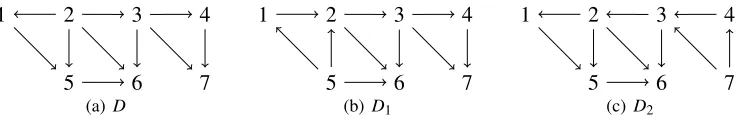
Definition 5 (Intervention graph) Let D= ([p],E) be a DAG with vertex set[p]and edge set E (see Appendix A.1), and I⊂[p]an intervention target. The intervention graphof D is the DAG D(I)= ([p],E(I)), where E(I):={(a,b)|(a,b)∈E,b∈/I}.
For a causal model(D,f), an interventional density f(·|doD(XI=UI))obeys the Markov property
ofD(I): the Markov property of the observational density is inherited. Figure 1 shows an example of a DAG and two corresponding intervention graphs.
As foreshadowed in the introduction, we are interested in causal inference based on data sets originating frommultipleinterventions, that means from a set of the formS={(Ij,f˜j)}Jj=1, where
Ij⊂[p]is an intervention target and ˜fj a level density onXIj for 1≤ j≤J. We call such a set an intervention setting, and the corresponding (multi)set of intervention targetsI={Ij}Jj=1afamily of targets. We often use the family of targets as an index set, for example to write a corresponding intervention setting asS={(I,fI˜)}I∈I.
We considerinterventional dataof sample sizenproduced by a causal model(D,f)under an
intervention settingS={(I,f˜I)}I∈I. We assume that thensamplesX(1), . . . ,X(n)are independent,
and write them as usual as rows of adata matrix X. However, they arenotidentically distributed
1 2 3 4
5 6 7
(a)D
1 2 3 4
5 6 7
(b)D({4})
1 2 3 4
5 6 7
(c) D({3,5})
as they arise fromdifferentinterventions. The interventional data set is fully specified by the pair (T,X),
T =
T(1)
.. .
T(n)
∈ I
n, X=
—X(1)— .. . —X(n)—
, (2)
where for eachi∈[n],T(i)denotes the intervention target under which the sampleX(i)was produced. This data set can potentially contain observational data as well, namely if/0∈ I. To summarize, we consider the statistical model
X(1),X(2), . . . ,X(n)independent,
X(i)∼ f · | doD(XT(i()i)=UT(i))
,UT(i) ∼ f˜T(i), i=1, . . . ,n, (3)
and we assume that each targetI∈ I appears at least once in the sequenceT.
2.2 Interventional Markov Equivalence: New Concepts and Results
An intervention at some target a∈[p]destroys the original causal influence of other variables of the system onXa. Interventional data thereof can hence not be used to determine the causal parents ofXain the (undisturbed) system. To be able to estimate at least the complete skeleton of a causal
structure (as in the observational case), an intervention experiment has to be performed based on a
conservativefamily of targets:
Definition 6 (Conservative family of targets) A family of targetsIis calledconservativeif for all a∈[p], there is some I∈ I such that a∈/I.
In this paper, we restrict our considerations toconservativefamilies of targets; see Section 2.3 for a more detailed discussion. Note that every experiment in which we also measure observational data corresponds to a conservative family of targets.
If a family of targets I contains more than one target, interventional data as in Equation (3)
arenot identically distributed. Whereas the distribution of observational data is determined by a
singledensity, we needtuplesof densities as in the following definition to specify the distribution of interventional data.
Definition 7 Let D be a DAG on[p], and letIbe a family of targets. Then we define MI(D):=
(f(I))I∈I∈ M|I|
∀I∈ I: f(I)∈ M(D(I)), and
∀I,J∈ I,∀a∈/I∪J: f(I)(xa|xpaD(a)) = f
(J)(xa|x
paD(a)) .
Lemma 8 Let D be a DAG on[p], andIa conservative family of targets.
(i) Let(D,f) be a causal model (that is, f ∈ M(D)),S={(I,f˜I)}I∈I an intervention setting
and UI∼ f˜Iintervention variables for I∈ I. Then, we have f(· |do(XI=UI))
I∈I∈ MI(D).
(ii) Let(f(I))I∈I∈ MI(D). Then there is some positive density f ∈ M(D)and an intervention
settingS={(I,fI˜)}I∈I such that f(·|do(XI =UI)) = f(I)(·) for random variables UI with
density fI, for all I˜ ∈ I.
Definition 9 (Interventional Markov equivalence) Let D1 and D2 be DAGs, and I a family of
targets. D1and D2are calledI-Markov equivalent(notation: D1∼ID2) ifMI(D1) =MI(D2).
TheI-Markov equivalence class of a DAG D is denoted by[D]I.
Alternatively, we will also use the term “interventionally Markov equivalent” when it is clear which family of targets is meant. For the simplest conservative family of targets,I ={/0}, we get back Definition 2 for the observational case. We now generalize Theorem 3 for the interventional case in order to get a purely graph theoretic criterion for interventional Markov equivalence of two given DAGs, the main result of this section.
Theorem 10 Let D1and D2be two DAGs on[p], andIa conservative family of targets. Then, the
following statements are equivalent:
(i) D1∼ID2;
(ii) for all I∈ I, D(1I)∼D(2I)(in the observational sense);
(iii) for all I∈ I, D(1I)and D(2I)have the same skeleton and the same v-structures; (iv) D1and D2have the same skeleton and the same v-structures, and D(1I)and D
(I)
2 have the same
skeleton for all I∈ I.
2.3 Discussion
Throughout this paper, we always assume the observational density fof a causal model to be strictly positive. This assumption makes sure that the conditional densities in Equation (1) are well-defined. The requirement of a strictly positive density can, however, be a restriction for example for discrete models (where the density is with respect to the counting measure). In the observational case, the notion of Markov equivalence remains the same when we also allow densities that are not strictly positive (Lauritzen, 1996). We conjecture that the notion of interventional Markov equivalence (Definition 9 and Theorem 10) also remains valid for such densities; corresponding proofs would, however, require more caution to avoid the aforementioned problems with (truncated) factorization. To illustrate the importance of a conservative family of targets for structure identification, let us consider the simplest non-trivial example of a causal model with 2 variablesX1 andX2. Under observational data, we can distinguish two Markov equivalence classes: one in which the variables
are independent (represented by the empty DAGD0), and one in which they are not independent
(represented by the DAGsD1:=1 2 andD2:=1 2). D1andD2 can be distinguished if we
1 2 3 4
5 6 7
(a) D
1 2 3 4
5 6 7
(b)D1
1 2 3 4
5 6 7
(c)D2
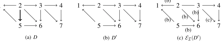
Figure 2: Three DAGs having equal skeletons and a single v-structure, 3 6 5, hence being
observationally Markov equivalent. ForI={/0,{4}}, we haveD∼ID1, butD6∼ID2 since the skeletons ofD({4})(Figure 1(b)) andD({24})do not coincide.
intervention at, say, X1 alone(that is, in the absenceof observational data), corresponding to the
non-conservative familyI={{1}}, only allows a distinction between the models D2 andD0 on
the one hand (which do not show dependence betweenX1 andX2 under the intervention) andD1
on the other hand (which does show dependence betweenX1 andX2 under the intervention). Note
that the two indistinguishable modelsD0 andD2 do not even have the same skeleton, and that it
is impossible to determine the influence ofX2on X1 in the undisturbed system. In this setting, it
would be more natural to consider the intervened variableX1 as an external parameter rather than
a random variable of the system, and to perform regression to detect or determine the influence of
X1onX2. Note, however, that full identifiability of the models doesnotrequire observational data; interventions atX1andX2(corresponding to the conservative familyI={{1},{2}}in our notation) are also sufficient.
Theorem 10 is of great importance for the description of Markov equivalence classes under interventions. It shows that two DAGs which are interventionally Markov equivalent under some conservative family of targets are also observationally Markov equivalent:
D1∼I D2⇒D1∼D2. (4)
This implication isnottrue anymore for non-conservative families of targets. This is an explanation for the term “conservative”: a conservative family of targets yields a finer partitioning of DAGs into equivalence classes compared to observational Markov equivalence, but it preserves the “borders” of observational Markov equivalence classes. Figure 2 shows three DAGs that are observationally Markov equivalent, but which fall into two different interventional Markov equivalence classes under the family of targetsI={/0,{4}}.
Theorem 10 agrees with Theorem 3 of Tian and Pearl (2001) for single-variable interventions.
While we also make a statement about interventions atseveralvariables, they prove their theorem
for perturbations of the system at single variables only, but for a wider class of perturbations called mechanism changesthat go beyond our notion of interventions. While an intervention destroys the causal dependence of a variable from its parents (and hence replaces a conditional density by
a marginal one in the Markov factorization, see Equation (1)), a mechanism change(also known
3. Essential Graphs
Theorem 10 represents a computationally fast criterion for deciding whether two DAGs are interven-tionally Markov equivalent or not. However, given some DAGD, it does not provide a possibility for quickly findingallequivalent ones, and hence does not specify the equivalence class as a whole. In this section, we give a characterization of graphs that uniquely represent an interventional Markov equivalence class (Theorem 18). Our characterization of theseinterventional essential graphsis in-spired by and similar to the one developed by Andersson et al. (1997) for the observational case and allows for handling equivalence classes algorithmically. Furthermore, we present a linear time al-gorithm for constructing a representative of the equivalence class corresponding to an interventional essential graph (Proposition 16 and discussion thereafter), as well as a polynomial time algorithm for constructing the interventional essential graph of a given DAG (Algorithm 1). Throughout this section,Ialways stands for a conservative family of targets.
3.1 Definitions and Motivation
All DAGs in anI-Markov equivalence class share the same skeleton; however, arrow orientations
may vary between different representatives (Theorem 10). Varying and common arrow orientations are represented by undirected and directed edges, respectively, inI-essential graphs.
Definition 11 (I-essential graph) Let D be a DAG. The I-essential graph of D is defined as EI(D):=SD′∈[D]
ID
′. (The union is meant in the graph theoretic sense, see Appendix A.1).
When the family of targets I in question is clear from the context, we will also use the term
in-terventional essential graph, while “observational essential graph” shall refer to the concept of essential graphs as introduced by Andersson et al. (1997) in the observational case. Simply speak-ing of “essential graphs”, we mean interventional or observational essential graphs in the followspeak-ing.
Definition 12 (I-essential arrow) Let D be a DAG. An edge a b∈D isI-essentialin D if a b∈D′∀D′∈[D]I.
AnI-essential graph typically contains directed as well as undirected edges. Directed ones corre-spond to arrows that areI-essential in every representative of the equivalence class; in other words,
I-essential arrows are those whose direction is identifiable. A first sufficient criterion for an edge
to beI-essential follows immediately from Lemma 47 (Appendix B.1).
Corollary 13 Let D be a DAG with a b∈D. If there is an intervention target I∈ I such that |{a,b} ∩I|=1, then a b isI-essential.
The investigation of essential graphs has a long tradition in the observational case (Anders-son et al., 1997; Chickering, 2002a). Due to increased identifiability of causal structures, Markov equivalence classes shrink in the interventional case; Equation (4) impliesEI(D)⊂ E{/0}(D)for any conservative family of targetsI(see also Figure 8 in Section 5). Essential graphs, interventional as well as observational ones, are mainly interesting because of two reasons:
• It is important to know which arrow directions of a causal model are identifiable and which
1 2 3 4
5 6 7
(d) (b)
(b)
(c)
Figure 3: A graph with six arrows. Four of them are strongly I-protected for any conservative
family of targets I (in parentheses: arrow configurations according to Definition 14).
Arrows 3 4 and 4 7 are stronglyI-protected forI={/0,{4}}, but not forI={/0}.
• Markov equivalent DAGs encode the same statistical model. Hence the space of DAGs is
no suitable “parameter” or search space for statistical inference and computation. The natural search space is given by the set of the equivalence classes, the objects that can be distinguished from data. Essential graphs uniquely represent these equivalence classes and are efficiently manageable in algorithms.
The characterization of I-essential graphs (Theorem 18) relies on the notion of stronglyI
-protected arrows (Definition 14) which reproduces the corresponding definition of Andersson et al. (1997) forI={/0}; an illustration is given in Figure 3.
Definition 14 (Strong protection) Let G be a graph. An arrow a b∈G isstronglyI-protected
in G if there is some I∈ Isuch that|I∩ {a,b}|=1, or the arrow a b occurs in at least one of the following four configurations as an induced subgraph of G:
(a): a b
c
(b): a b
c
(c): a b
c
(d): a b
c1
c2
We will see in Theorem 18 that every arrow of anI-essential graph (that is, every edge corre-sponding to anI-essential arrow in the representative DAGs) is stronglyI-protected. The config-urations in Definition 14 guarantee the identifiability of the edge orientation between a andb: if there is a targetI∈ Isuch that|I∩ {a,b}|=1, turning the arrow would change the skeleton of the intervention graph D(I) (see also Corollary 13); in configuration (a), reversal would create a new v-structure; in (b), reversal would destroy a v-structure; in (c), reversal would create a cycle; an
in (d) finally, at least one of the arrows between aand c1 or c2 must point away from a in each
representative, hence turning the arrowa bwould create a cycle. We refer to Andersson et al.
(1997) for a more detailed discussion of the configurations (a) to (d).
3.2 Characterization of Interventional Essential Graphs
As in the observational setting, we can show that interventional essential graphs are chain graphs
with chordal chain components (see Appendix A.1). For the observational caseI ={/0},
Proposi-tions 15 and 16 below correspond to ProposiProposi-tions 4.1 and 4.2 of Andersson et al. (1997).
Proposition 15 Let D be a DAG on[p]. Then:
(ii) For each chain component T∈T(EI(D)), the induced subgraphEI(D)[T]is chordal.
Proposition 16 Let D be a DAG. A digraph D′ is acyclic andI-equivalent to D if and only if D′ can be constructed by orienting the edges of every chain component ofEI(D)according to a perfect
elimination ordering.
This proposition is not only of theoretic, but also of algorithmic interest. According to the expla-nation in Appendix A.2, perfect elimiexpla-nation orderings on the (chordal) chain components ofEI(D)
can be generated withLexBFS(Algorithm 6); doing this for all chain components yields
compu-tational complexityO(|E|+p), whereE denotes the edge set ofEI(D)(see Appendix A.2). As an immediate consequence of Proposition 16, interventional essential graphs are in one-to-one correspondence with interventional Markov equivalence classes. We will therefore also speak
about “representatives of I-essential graphs”, where we mean representatives (that is, DAGs) of
the corresponding equivalence class. Propositions 15 and 16 give the justification for the following definition; note that in order to generate a representative of someI-essential graph, the family of
targetsI need not be known.
Definition 17 Let G be the I-essential graph of some DAG. The set of representatives of G is denoted byD(G):
D(G):={D a DAG|D⊂G,Du=Gu,D[T]oriented according to some perfect elimination ordering for each chain component T ∈T(G)}.
Here,Dudenotes the skeleton ofD(Appendix A.1). We can now state the main result of this section, a graph theoretic characterization ofI-essential graphs. For the observational case I={/0}, this theorem corresponds to Theorem 4.1 of Andersson et al. (1997).
Theorem 18 A graph G is theI-essential graph of a DAG D if and only if (i) G is a chain graph;
(ii) for each chain component T ∈T(G), G[T]is chordal; (iii) G has no induced subgraph of the form a b c;
(iv) G has no line a b for which there exists some I∈ Isuch that|I∩ {a,b}|=1; (v) every arrow a b∈G is stronglyI-protected.
The graph Gof Figure 3 satisfies points (i) to (iii) of Theorem 18. For I ={/0,{4}}, it also fulfills points (iv) and (v); in this case, it is theI-essential graphEI(D)of the DAGDof Figure 1(a) by Proposition 16.
3.3 Construction of Interventional Essential Graphs
In this section, we show that there is a simple way to construct theI-essential graphEI(D)of a DAG
D: we need to successively convert arrows that are not stronglyI-protected into lines (Algorithm 1). By doing this, we get a sequence of partialI-essential graphs.
Definition 19 (PartialI-essential graph) Let D be a DAG. A graph G with D⊂G⊂ EI(D) is
The following lemma can be understood as a motivation for looking at such graphs. Note that due to the conditionG⊂ EI(D), and becauseGandEI(D)have the same skeleton, every arrow ofEI(D) is also present inG, hence statement (ii) below makes sense.
Lemma 20 Let D be a DAG. Then:
(i) D andEI(D)are partialI-essential graphs of D.
(ii) Let G be a partialI-essential graph of D. Every arrow a b∈ EI(D)is stronglyI-protected
in G.
(iii) Let G be a partialI-essential graph of two DAGs D1and D2. Then, D1∼I D2.
Algorithm 1 constructs the I-essential graph Gfrom a partialI-essential graph of any DAG
D∈D(G). The algorithm is indeed valid and calculatesEI(D), since the graph produced in each iteration is a partialI-essential graph ofD(Lemma 21), and the only partialI-essential graph that has only stronglyI-protected arrows isEI(D)(Lemma 22).
Lemma 21 Let D be a DAG and G a partialI-essential graph of D. Assume that a b∈G is not stronglyI-protected in G, and let G′:=G+ (b,a)(that is, the graph we get by replacing the arrow a b by a line a b; see Appendix A.1). Then G′is also a partialI-essential graph of D.
Lemma 22 Let D be a DAG. There is exactly one partialI-essential graph of D in which every arrow is stronglyI-protected, namelyEI(D).
To constructEI(D)from some DAGD= ([p],E), we must, in the worst case, execute the itera-tion of Algorithm 1 for every arrow in the DAG; at each step, we must check every 4-tuple of vertices to see whether some arrow occurs in configuration (d) of Definition 14. Therefore Algorithm 1 has at most complexity O(|E| ·p4); by exploiting the partial orderG onT(G)(see Appendix A.1),
more efficient implementations are possible. Note that some checks only need to be done once. If, for example, an edgea bis part of a v-structure (configuration (b) of Definition 14), or if there is someI∈ I such that|I∩ {a,b}|=1 in the first iteration of Algorithm 1, this will also be the case in every later iteration.
3.4 Example: Identifiability under Interventions
A simple example illustrates how much identifiability can be gained with a single intervention. We consider a linear chain as observational essential graph:
G=E{/0}(D): 1 2 3 · · · p.
We can easily count the number of representatives ofGusing the following lemma.
Input :G: partialI-essential graph of some DAGD(not known) Output:EI(D)
while∃a b∈G s.t. a b not stronglyI-protected in Gdo
G←G+ (b,a);
returnG;
Lemma 23 (Source lemma) Let G be a connected, chordal, undirected graph, and let D⊂G be a DAG without v-structures and with Du=G. Then D has exactly one source.
Proof Let σ be a topological ordering of D; then, σ(1) is a source, see Appendix A.1. It re-mains to show that there is at most one such source. Assume, for the sake of contradiction, that there are two different sources u and v. Since G is connected, there is a shortest u-v-path
γ= (a0≡u,a1, . . . ,ak ≡v). Let ai ai+1∈Dbe the first arrow that points away fromv in the
chainγinD(notei≥1 sinceu a1∈Dby assumption). The v-structureai−1 ai ai+1is not
allowed as an induced subgraph ofD, henceai−1andai+1must be adjacent inDand inG; however,
γis then noshortest u-v-path, a contradiction.
For our linear chainGand anys∈[p], there is exactly one DAGD∈D(G)that has the (unique)
sources, namely the DAG we get by orientingalledges ofGaway froms; other edge orientations
would produce a v-structure. We concludeGhasprepresentatives.
Assume that the true causal model producing the data is (D,f), and denote the source of D
by s∈[p]. Consider the conservative family of targets I ={/0,{v}} with v∈[p]. If v<s, the interventional essential graphEI(D)is
1 2 . . . v+1 . . . p,
and|D(EI(D))|=p−vby the same arguments as above; analogously, ifv>s, we find|D(EI(D))|=
v−1. On the other hand, ifv=s, all edges ofDare stronglyI-protected: those incident tosbecause of the intervention target, all others because they are in configuration (a) of Definition 14; therefore, we haveEI(D) =D.
In the best case, all edge orientations in the chain can be identified by a single intervention, while the observational essential graph E{/0}(D) that is identifiable from observational data alone
contains prepresentatives. However, this needs an intervention at the a priori unknown source s.
Choosing the central vertex⌈p2⌉as intervention target ensures that at least half of the edges become directed inEI(D), independent of the positionsof the source.
4. Greedy Interventional Equivalence Search
Different algorithms have been proposed to estimate essential graphs from observational data. One of them, the Greedy Equivalence Search (GES) (Meek, 1997; Chickering, 2002b), is particularly interesting because of two properties:
• It is score-based; it greedily maximizes some score function for given data over essential
graphs. It uses no tuning-parameter; the score function alone measures the quality of the estimate. Chickering (2002b) chose the BIC score because of consistency; technically, any score equivalent and decomposable function (see Definition 24) is adequate.
• It traverses the space of essential graphs which is the natural search space for model inference (see Section 3). We will see in Section 5 that a greedy search overequivalence classesyields much better estimation results than a na¨ıve greedy search overDAGs.
• In theforward phase, the algorithm starts with the empty essential graph, G0:= ([p],/0). It then sequentially steps from one essential graphGito alargerone,Gi+1, for which there are representativesDi∈D(Gi)andDi+1∈D(Gi+1)such thatDi+1 has exactly one arrow more thanDi.
• In the backward phase, the sequence (Gi)i is continued by gradually stepping from one
essential graphGito asmallerone,Gi+1, for which there are representativesDi∈D(Gi)and
Di+1∈D(Gi+1)such thatDi+1has exactly one arrow less thanDi.
In both phases, the respective candidate with maximal score is chosen, or the phase is aborted if no candidate scores higher than the current essential graphGi.
We introduce in addition a new turning phase which proved to enhance estimation (see Section 5). Here, the sequence(Gi)iis elongated by gradually stepping from one essential graphGito a new
one with the same number of edges, denoted byGi+1, for which there are representativesDi∈D(Gi)
andDi+1∈D(Gi+1) such thatDi+1can be constructed from Di by turning exactly one arrow. As before, we choose the highest scoring candidate. Such a turning phase had already been proposed, but not characterized or implemented, by Chickering (2002b).
Because GES is an optimization algorithm working on the space of observational essential graphs, and because the characterization ofinterventionalessential graphs is similar to that of ob-servational ones (Theorem 18), GES can indeed be generalized to handle interventional data as well by operating on interventional instead of observational essential graphs. We call this generalized
algorithmGreedy Interventional Equivalence Searchor GIES. An overview is shown in Algorithm
2: the forward, backward and turning phase are repeatedly executed in this order until none of them can augment the score function any more.
A na¨ıve search strategy would perhaps traverse the space of DAGs instead of essential graphs, greedily adding, removing or turning single arrows from DAGs. It is well-known in the observa-tional case that such an approach performs markedly worse than one accounting for Markov equiv-alence (Chickering, 2002b; Castelo and Koˇcka, 2003), and we will see in our simulations (Section 5.2) that the same is true in the interventional case as long as few interventions are made. Ignoring Markov equivalence cuts down the search space of successors at haphazard; since all DAGs in a Markov equivalence class represent the same statistical model, there is no justification for consider-ing neighbors (that is, DAGs that can be reached by addconsider-ing, removconsider-ing or turnconsider-ing an arrow) of one of the representatives but not of the other ones.
GIES can be used with general score functions. It goes without saying that the chosen score function should be a “reasonable” one which has favorable statistical properties such as consistency. We denote the score of a DAGDgiven interventional data(T,X)by S(D;T,X), and we assume thatSisscore equivalent, that is, it assigns the same score toI-equivalent DAGs;Ialways stands for a conservative family of targets in this section. Furthermore, we requireSto be decomposable.
Definition 24 A score function S is calleddecomposableif for each DAG D, S can be written as a sum
S(D;T,X) =
p
∑
i=1
s(i,paD(i);T,X),
where thelocal scores depends onXonly viaXiandX paD(i), withX idenoting the i
Throughout the rest of this section,Salways denotes a score equivalent and decomposable score function. Such a score function needs only be evaluated at one single representative of some inter-ventional Markov equivalence class. Indeed, a key ingredient for the efficiency of the observational GES as well as our interventional GIES is an implementation that computes the greedy steps to the next equivalence class in a local fashion without enumerating all corresponding DAG members. Chickering (2002b) found a clever way to do that in the forward and backward phase of the obser-vational GES. In Sections 4.1 and 4.2, we generalize his methods to the interventional case, and in Section 4.3, we propose an efficient implementation of the new turning phase.
4.1 Forward Phase
A step in the forward phase of GIES can be formalized as follows: for anI-essential graphGi, find
the next oneGi+1:=EI(Di+1), where
Di+1:= arg max
D′∈D+(G
i)
S(D′;T,X), and
D+(Gi):={D′a DAG| ∃an arrowu v∈D′:D′−(u,v)∈D(Gi)}.
If no candidate DAGD′∈D+(Gi)scores higher thanGi, abort the forward phase.
We denote the set of candidateI-essential graphs byEEE+I(Gi):={EI(D′)|D′∈D+(Gi)}. In
the next proposition, we show that each graphG′∈ EEE+I(Gi)can be characterized by a triple(u,v,C),
whereu vis the arrow that has to be added to a representative DofGi in order to get a
repre-sentativeD′ ofG′, andCspecifies the edge orientations ofDwithin the chain component of vin
G.
Input :(T,X): interventional data for family of targetsI
Output:I-essential graph
G←([p],/0); repeat
DoContinue←FALSE; repeat
Gold←G;
G←ForwardStep(G;T,X); // See Algorithm 3 untilGold=G;
repeat
Gold←G;
G←BackwardStep(G;T,X); // See Algorithm 4 ifGold6=GthenDoContinue←TRUE;
untilGold=G; repeat
Gold←G;
G←TurningStep(G;T,X); // See Algorithm 5
ifGold6=GthenDoContinue←TRUE; untilGold=G;
until¬DoContinue;
Proposition 25 Let G be anI-essential graph, let u and v be two non-adjacent vertices of G, and let C⊂neG(v). Then there is a DAG D∈D(G) with {a∈neG(v)|a v∈D}=C such that D′:=D+ (u,v)∈D+(G)if and only if
(i) C is a clique in G[TG(v)]; (ii) N:=neG(v)∩adG(u)⊂C;
(iii) and every path from v to u in G has a vertex in C.
For given G, u, v and C determine D′uniquely up toI-equivalence.
Note that points (i) and (ii) imply in particular thatN is a clique in G[TG(v)]. Proposition 25 has
already been proven for the case of observational data (Chickering, 2002b, Theorem 15); it is not obvious, however, to see that this characterization of a forward step is also valid for interventional essential graphs, so we give a new proof in Appendix B.3 using the results developed in Sections 2 and 3.
The DAGsDandD′ in Proposition 25 only differ in the edge(u,v);vis the only vertex whose
parents are different inDandD′. Since the score functionSis assumed to be decomposable, the
score difference betweenDandD′can be expressed by the local score change at vertexv, as stated in the following corollary.
Corollary 26 Let G, u, v, C, D and D′ be as in Proposition 25. The score difference ∆S :=
S(D′;T,X)−S(D;T,X)can be calculated as follows:
∆S=s(v,paG(v)∪C∪ {u};T,X)−s(v,paG(v)∪C;T,X).
In the observational case, this corollary corresponds to Corollary 16 of Chickering (2002b).
Input :G= ([p],E):I-essential graph;(T,X): interventional data forI
Output:G′∈ EEE+I(G), orG
∆Smax←0;
2 foreachv∈[p]do
foreachu∈[p]\adG(v)do
N←neG(v)∩adG(u);
foreachclique C⊂neG(v)with N⊂Cdo // Proposition 25(i) and (ii) if6 ∃path from v to u in G[[p]\C]then // Proposition 25(iii)
∆S←s(v,paG(v)∪C∪ {u};T,X)−s(v,paG(v)∪C;T,X);
if∆S>∆Smaxthen
∆Smax←∆S;
10 (umax,vmax,Cmax)←(u,v,C);
if∆Smax>0then
σ←LexBFS((Cmax,vmax, . . .),E[TG(vmax)]); Orient edges ofG[TG(vmax)]according toσ; Insert edge(umax,vmax)intoG;
returnReplaceUnprotected(I,G); // See Algorithm 1 else returnG;
1 2 3 4
5 6 7
(a) D
1 2 3 4
5 6 7
(b)D′
1 2 3 4
5 6 7
(a) (b)
(a)
(c) (b)
(b) (c)
(c)EI(D′)
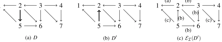
Figure 4: DAGs D, D′ andEI(D′)illustrating a possible forward step of GIES for the family of targetsI ={/0,{4}}, applied to theI-essential graphGof Figure 3 for the parameters (u,v,C) = (4,2,{3}) (notation according to Proposition 25). In parentheses in Figure (c): arrow configurations according to Definition 14; arrows incident to 4 are strongly
I-protected by the intervention target{4}.
The most straightforward way to construct an I-essential graphG′∈ EEE+I(G)characterized by the triple (u,v,C) as defined in Proposition 25 would be to create a representative D∈D(G) by orienting the edges of TG(v)as indicated by the setC, add the arrowu v to getD′, and finally
constructEI(D′)with Algorithm 1. The next lemma suggests a novel shortcut to this procedure: it is sufficient to orient the edges of the chain componentTG(v)onlyto get a partialI-essential graph ofD′after adding the arrowu v.
Lemma 27 Let G, u, v, C, D and D′ be as in Proposition 25. Let H be the graph that we get by orienting all edges of TG(v)as in D (leaving other chain components unchanged) and inserting the arrow(u,v). Then H is a partialI-essential graph of D′.
Algorithm 3 shows our implementation of the forward phase of GIES, summarizing the results of Proposition 25, Corollary 26 and Lemma 27. Figure 4 illustrates one forward step, applied to theI-essential graphG(forI={/0,{4}}) of Figure 3 and characterized by the triple (u,v,C) = (4,2,{3}). Note that this triple is indeed valid in the sense of Proposition 25: {3}is clearly a clique (point (i)), neG(2)∩adG(4) ={3}(point (ii)), and there is no path from 2 to 4 inG[[p]\C](point
(iii)).
4.2 Backward Phase
In analogy to the forward phase, one step of the backward phase can be formalized as follows: for anI-essential graphGi, find its successorGi+1:=EI(Di+1), where
Di+1:= arg max
D′∈D−(G
i)
S(D′;X), and
D−(Gi):={D′a DAG| ∃D∈D(Gi),u v∈D:D′=D−(u,v)}.
If no candidate DAGD′∈D+(Gi)scores higher thanGi, the backward phase is aborted.
Whenever we have some representative D∈D(G)of an I-essential graphG, we get a DAG
inD−(G)by removing any arrow ofD. This is in contrast to the forward phase where we do not
In Proposition 28 (corresponding to Theorem 17 of Chickering (2002b) for the observational
case), we show that we can, similarly to the forward phase, characterize an I-essential graph of
EEE−I(G):={EI(D′)|D′ ∈D−(G)} by a triple(u,v,C), where C is a clique in neG(v). As in the
forward phase, we see that the score difference ofDandD′is determined by the local score change at the vertexv(Corollary 29), and that lines in chain components other thanTG(v) remain lines in G′=EI(D′)(Lemma 30). Algorithm 4 summarizes the results of the propositions in this section. Proposition 28 Let G= ([p],E) be an I-essential graph with(u,v)∈E (that is, u v∈G or u v∈G), and let C⊂neG(v). There is a DAG D∈D(G) with u v∈D and{a∈neG(v)\ {u} |a v∈D}=C such that D′:=D−(u,v)∈D−(G)if and only if
(i) C is a clique in G[TG(v)]; (ii) C⊂N:=neG(v)∩adG(u).
Moreover, u, v and C determine D′uniquely up toI-equivalence for a given G.
Corollary 29 Let G, u, v, C, D and D′ be as in Proposition 28. The score difference ∆S :=
S(D′;T,X)−S(D;T,X)is:
∆S=s(v,(paG(v)∪C)\ {u};T,X)−s(v,paG(v)∪C∪ {u};T,X).
In the observational case, this corresponds to Corollary 18 in Chickering (2002b). The analogue to Lemma 27 for a computational shortcut in the forward phase reads as follows:
Lemma 30 Let G, u, v, C, D and D′ be as in Proposition 28. Let H be the graph that we get by orienting all edges of TG(v)as in D and removing the arrow(u,v). Then H is a partialI-essential graph of D′.
Input :G= ([p],E):I-essential graph;(T,X): interventional data forI
Output:G′∈ EEE−I(G), orG
∆Smax←0;
foreachv∈[p]do
foreachu∈neG(v)∪paG(v)do N←neG(v)∩adG(u); foreachclique C⊂Ndo
∆S←s(v,(paG(v)∪C)\ {u};T,X)−s(v,paG(v)∪C∪ {u};T,X); if∆S>∆Smaxthen
∆Smax←∆S;
(umax,vmax,Cmax)←(u,v,C); if∆Smax>0then
ifumax∈neG(vmax)thenσ←LexBFS((Cmax,umax,vmax, . . .),E[TG(vmax)]); elseσ←LexBFS((Cmax,vmax, . . .),E[TG(vmax)]);
Orient edges ofG[TG(vmax)]according toσ; Remove edge(umax,vmax)fromG;
returnReplaceUnprotected(I,G); // See Algorithm 1 else returnG;
1 2 3 4
5 6 7
(a) D
1 2 3 4
5 6 7
(b)D′
1 2 3 4
5 6 7
(b)
(b) (b)
(b)
(b) (c)
(c)EI(D′)
Figure 5: DAGsD,D′andEI(D′)illustrating a possible backward step of GIES for the family of targetsI ={/0,{4}}, applied to the I-essential graphGof Figure 3 for the parameters (u,v,C) = (2,5,/0) (notation according to Proposition 28). Figure (c), in parentheses: arrow configurations according to Definition 14.
A backward step of GIES is summarized in Algorithm 4 and illustrated in Figure 5. The triple (u,v,C) = (2,5,/0)used there to characterize the backward step obviously fulfills the requirements of Proposition 28.
4.3 Turning Phase
Finally, we characterize a step of the turning phase of GIES, in which we want to find the successor
Gi+1:=EI(Di+1)for anI-essential graphGiby the rule Di+1:=arg max
D′∈D (G
i)
S(D′;T,X),where
D (Gi):={D′ a DAG|D′∈/D(Gi),and∃an arrowu v∈D′:
D′−(u,v) + (v,u)∈D(Gi)}.
When the score cannot be augmented anymore, the turning phase is aborted. The additional con-dition “D′ ∈/ D(Gi)” is not necessary in the definitions of D+(Gi) andD−(Gi); when adding or
removing an arrow from a DAG, the skeleton changes, hence the new DAG is certainly not I
-equivalent to the previous one. However, whenturning an arrow, the skeleton remains the same,
and the danger of staying in the same equivalence class exists.
Again, we are looking for an efficient method to find a representativeD′for eachG′∈ EEEI(Gi):= {EI(D′)|D′∈D (Gi)}. It makes sense to distinguish whether the arrow that should be turned in
a representativeD∈D(Gi)isI-essential or not. We start with the case where we want to turn an arrow which isnotI-essential.
Proposition 31 Let G be an I-essential graph with u v∈G, and let C⊂neG(v)\ {u}. Define N:=neG(v)∩adG(u). Then there is a DAG D∈D(G)with u v∈D and{a∈neG(v)|a v∈ D}=C such that D′:=D−(v,u) + (u,v)∈D (G)if and only if
(i) C is a clique in G[TG(v)]; (ii) C\N6=/0;
(iii) C∩N separates C\N and N\C in G[neG(v)].
1 2 3 4
5 6 7
(a) D
1 2 3 4
5 6 7
(b)D′
1 2 3 4
5 6 7
(a)
(c)
(b)
(b) (b)
(b) (c)
(c)EI(D′)
Figure 6: DAGs D, D′ andEI(D′) illustrating a possible turning step of GIES applied to theI -essential graph G (I ={/0,{4}}) of Figure 3 for the parameters (u,v,C) = (5,2,{3}) (notation of Proposition 31). The arrow 2 5 is notI-essential inD. Figure (c): arrow configurations in parentheses, see Definition 14.
There are nowtwovertices that have different parents in the DAGsDandD′, namelyuandv; thus the calculation of the score difference betweenDandD′ involves two local scores instead of one.
Corollary 32 Let G, u, v, C, D and D′ be as in Proposition 31. Then the score difference∆S:=
S(D′;T,X)−S(D;T,X)can be calculated as follows:
∆S=s(v,paG(v)∪C∪ {u};T,X) +s(u,paG(u)∪(C∩N);T,X) −s(v,paG(v)∪C;T,X)−s(u,paG(u)∪(C∩N)∪ {v};T,X).
Lemma 33 Let G, u, v, C, D and D′ be as in Proposition 31. Let H be the graph that we get by orienting all edges of TG(v)as in D and turning the arrow (v,u). Then H is a partialI-essential graph of D′.
A possible turning step is illustrated in Figure 6, where a non-I-essential arrow (for I =
{/0,{4}}) of a representative of the graph G of Figure 3 is turned. The step is characterized by the triple(u,v,C) = (5,2,{3})which satisfies the conditions of Proposition 31: {3}is obviously a clique (point (i)),C\N=CsinceN={1}(point (ii)), andC\N={3}andN\C={1}are separated inG[neG(2)](point (iii)). In contrast, the triple(u,v,C) = (5,2,{1}) fulfills points (i) and (iii) of
Proposition 31, but not point (ii). There is a DAGD∈D(G)with{a∈neG(2)|a 2∈D}={1},
and turning the arrow 2 5 inDyields another DAGD′(that is, does not create a new cycle). This
new DAGD′, however, isI-equivalent toD, and hence not a member ofD (G)(see the discussion above).
We now proceed to the case where anI-essential arrow of a representative ofGis turned; here there is no danger to remain in the same Markov equivalence class. The characterization of this case is similar to the forward phase.
Proposition 34 Let G be anI-essential graph with u v∈G, and let C⊂neG(v). Then there is a DAG D∈D(G)with{a∈neG(v)|a v∈D}=C such that D′:=D−(v,u) + (u,v)∈D (G)if and only if
(i) C is a clique;
(ii) N:=neG(v)∩adG(u)⊂C;
1 2 3
4 5
(a) G
1 2 3
4 5
(b)D
1 2 3
4 5
(b) (b)
(c) (b)
(b)
(c)D′=EI(D′)
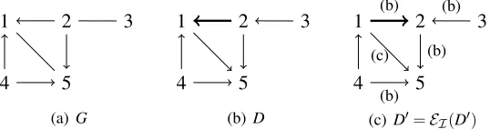
Figure 7: GraphsG, D, D′ andEI(D′) illustrating a possible turning step of GIES for the family of targetsI={/0,{4}}and the parameters(u,v,C) = (1,2,{3})(notation of Proposition 34). The arrow 2 1 isI-essential inD. Figure (c): arrow configurations in parentheses, see Definition 14.
Chickering (2002a) has already proposed a turning step for essential arrows in the observational case; however, he did not provide necessary and sufficient conditions specifying all possible turning steps as Proposition 34 does.
Lemma 35 Let G, u, v, C, D and D′be as in Proposition 34, and let H be the graph that we get by orienting all edges of TG(v)and TG(u)as in D and by turning the edge(v,u). Then H is a partial I-essential graph of D′.
To construct aG′∈ EEEI(G)out ofG, we must possibly orienttwochain components ofGinstead of one (Lemma 35). In the example of Figure 7, we see that it is indeed not sufficient to orient the edges ofTG(v) alone in order to get a partialI-essential graph of G′. The arrow 1 5 is notI
-essential inD, hence 5∈TG(1). However, the same arrow isI-essential inD′and hence also present
inEI(D′).
Despite the fact that we need to orient the edges ofTG(v)andTG(u)to get a partialI-essential
graph ofD′,EI(D′)is nevertheless determined by the orientation of edges adjacent tov(determined by the cliqueC) alone. This comes from the fact that inD, defined as in Proposition 34, all arrows ofD[TG(u)]must point away fromu.
Corollary 36 Let G, u, v, C, D and D′ be as in Proposition 34. Then the score difference∆S:=
S(D′;T,X)−S(D;T,X)can be calculated as follows:
∆S = s(v,paG(v)∪C∪ {u};T,X) +s(u,paG(u)\ {v};T,X) −s(v,paG(v)∪C;T,X)−s(u,paG(u);T,X).
The entire turning step, for essential and non-essential arrows, is shown in Algorithm 5.
4.4 Discussion
Every step in the forward, backward and turning phase of GIES is characterized by a triple(u,v,C),
where u andv are different vertices andC is a clique in the neighborhood ofv. To identify the
highest scoring movement from oneI-essential graphGto a potential successor inEEE+I(G),EEE−I(G) orEEEI(G), respectively, one potentially has to examine all cliques in the neighborhood neG(v)of
all verticesv∈[p]. The time complexity of any (forward, backward or turning) step applied to an
ofG. By restricting GIES toI-essential graphs with a bounded vertex degree, the time complexity
of a step of GIES is polynomial in p; otherwise, it is in the worst case exponential. We believe,
however, that GIES is in practice much more efficient than this worst-case complexity suggests. Some evidence for this claim is provided by the runtime analysis of our simulation study, see Section 5.2.
A heuristic approach to guarantee polynomial runtime of a greedy search has been proposed by Castelo and Koˇcka (2003) for the observational case. Their Hill Climber Monte Carlo (HCMC) algorithm operates in DAG space, but to account for Markov equivalence, the neighborhood of a number of randomly chosen DAGs equivalent to the current one is scanned in each greedy step.
Input :G= ([p],E):I-essential graph;(T,X): interventional data forI
Output:G′∈ EEEI, orG
∆Smax←0;
foreachv∈[p]do
foreachu∈neG(v)do // Consider arrows that are not I-essential for turning
N←neG(u)∩adG(v);
foreachclique C⊂neG(v)\ {u}do // Proposition 31(i) ifC\N6=/0and{u,v}separates C and N\C in G[TG(v)]then
// Proposition 31(ii) and (iii)
∆S←s(v,paG(v)∪C∪ {u};T,X) +s(u,paG(u)∪(C∩N);T,X);
∆S←∆S−s(v,paG(v)∪C;T,X)−s(u,paG(u)∪(C∩N)∪ {v};T,X); if∆S>∆Smaxthen
∆Smax←∆S;
(umax,vmax,Cmax)←(u,v,C);
foreachu∈chG(v)do // Consider I-essential arrows for turning
N←neG(v)∩adG(u);
foreachclique C⊂neG(v)with N⊂Cdo // Proposition 34(i) and (ii) if6 ∃path from v to u in G[[p]\(C∪neG(u))]−(v,u)then // Proposition 34(iii)
∆S←s(v,paG(v)∪C∪ {u};T,X) +s(u,paG(u)\ {v};T,X);
∆S←∆S−s(v,paG(v)∪C;T,X)−s(u,paG(u);T,X);
if∆S>∆Smaxthen
∆Smax←∆S;
(umax,vmax,Cmax)←(u,v,C);
if∆Smax>0then
ifvmax umax∈Gthen
σu:=LexBFS((umax, . . .),E[TG(umax)]); Orient edges ofG[TG(umax)]according toσ;
σv:=LexBFS((Cmax,vmax, . . .),E[TG(vmax)]); elseσv:=LexBFS((Cmax,vmax,umax, . . .),E[TG(vmax)]); Orient edges ofG[TG(vmax)]according toσv;
Turn edge(vmax,umax)inG;
returnReplaceUnprotected(I,G); // See Algorithm 1 else returnG;
The equivalence class of the current DAG is explored by randomly turning “covered arrows”, that is, arrows whose reversal does not change the Markov property. In our (interventional) notation, an arrow is covered if and only if it isnotstronglyI-protected (Definition 14). By limiting the number of covered arrow reversals, a polynomial runtime is guaranteed at the cost of potentially lowering the probability of investigating a particular successor inEEE+I(G),EEEI−(G)orEEEI(G), respectively. HCMC hence enables a fine tuning of the trade-off between exploration of the search space and runtime, or between greediness and randomness.
The order of executing the backward and the turning phase seems somewhat arbitrary. In the analysis of the steps performed by GIES in our simulation study (Section 5.2), we saw that the turning phase can generally only augment the score when very few backward steps were executed before. For this reason, we believe that changing the order of the backward and the turning phase would have little effect on the overall performance of GIES.
As already discussed by Chickering (2002b) for the observational case, caching techniques can markedly speed up GES; the same holds for GIES. The basic idea is the following: in a forward step, the algorithm evaluates a lot of triples(u,v,C)to choose the best one,(umax,vmax,Cmax)(lines 1 to 9 in Algorithm 3). After performing the forward move corresponding to(umax,vmax,Cmax), many of the triples evaluated in the step before are still valid candidates for next step in the sense of Proposition 25 and lead to the same score difference as before (see Corollary 26). Caching those values avoids unnecessary reevaluation of possible forward steps. The same holds for the backward and the turning phase; since the forward step is most frequently executed, a caching strategy in this phase yields the highest speed-up though.
We emphasize that the characterization of “neighboring”I-essential graphs inEEE+I(G),EEE−I(G)or
EEEI(G), respectively, by triples(u,v,C)is of more general interest for structure learning algorithms, for example for the design of sampling steps of an MCMC algorithm. Also the beforementioned HCMC algorithm could be extended to interventional data by generalizing the notion of “covered arcs” using Definition 14.
The prime example of a score equivalent and decomposable score function is the Bayesian infor-mation criterion (BIC) (Schwarz, 1978) which we used in our simulations (Section 5). It penalizes the complexity of causal models by their number of free parameters (ℓ0penalization); this number is the sum of free parameters of the conditional densities in the Markov factorization (Definition 1), which explains the decomposability of the score. Using different penalties, for example,ℓ2 penal-ization, can lead to a non-decomposable score function. GIES can also be adapted to such score functions; the calculation of score differences becomes computationally more expensive in this case since it cannot be done in a local fashion as in Corollaries 26, 29, 32 and 36.
GIES only relies on the notion of interventional Markov equivalence, and on a score function that can be evaluated for a given class of causal models. As we mentioned in Section 2.1, we believe that interventional Markov equivalence classes remain unchanged for models that do not have a strictly positive density. For this reason it should be safe to also apply GIES to such a model class.
5. Experimental Evaluation
We evaluated the GIES algorithm on simulated interventional data (Section 5.2) and onin silico
In both cases, we restricted our considerations toGaussiancausal models as summarized in Section 5.1.
5.1 Gaussian Causal Models
Consider a causal model(D,f) with a Gaussian density of the formN(0,Σ). The observational Markov property of such a model translates to a set oflinearstructural equations
Xi=
p
∑
j=1
βi jXj+εi,εi
indep.
∼ N(0,σ2i), 1≤i≤p, (5)
whereβi j=0 if j∈/paD(i). When the DAG structureDis known, the covariance matrixΣcan be
parameterized by theweight matrix
B:= (βi j)ip,j=1∈B(D):={A= (αi j)∈Rp×p|αi j =0 if j∈/paD(i)}
that assigns a weight βi j to each arrow j i∈D, and the vector of error covariances σ2 :=
(σ2
1, . . . ,σ2p):
Σ=Cov(X) = (1−B)
−1diag(σ2)(
1−B)
−T. This is a consequence of Equation (5).
We always assume Gaussian intervention variablesUI (see Section 2.1). In this case, not only
the observational density f is Gaussian, but also the interventional densities f(x|doD(XI=UI)).
An interventional data set(T,X)as defined in Equation (2) then consists ofnindependent, but not identically distributed Gaussian samples.
We use theBayesian information criterion(BIC) as score function for GIES:
S(D;T,X):=sup{ℓD(B,σ2;T,X)|B∈B(D),σ2∈R>p0} −
kD
2 log(n),
whereℓDdenotes the log-likelihood of the density in Equation (3):
ℓD(B,σ2;T,X) := n
∑
i=1
logf X(i)|doD(XT(i()i) =UT(i))
(6)
=
n
∑
i=1 h
∑
j∈/T(i)
logf(X(ji)|Xpa(i)
D(j)) +
∑
j∈T(i)
log ˜f(X(ji))i
= −1
2
n
∑
i=1j∈/
∑
T(i)h logσ2
j+
1
σ2
j
X(ji)−BjX(i)
2i +C
= −1
2
p
∑
j=1 h
|{i| j∈/T(i)}|logσ2j+ 1
σ2
j i:j
∑
∈/T(i)
X(ji)−BjX(i)2
i +C,
where the constantCis independent of the parameters(B,σ2)of the model. Since Gaussian causal models with structureDare parameterized byB∈B(D)andσ2∈Rp
>0, we havekD=p+|E|free
parameters, whereE denotes the edge set ofD. It can be seen in Equation (6) that themaximum
The DAG ˆDmaximizing the BIC yields aconsistentestimator for the true causal structureDin the sense thatP[Dˆ ∼ID]→1 in the limitn→∞as long as the true density fisfaithfulwith respect toD, that is,everyconditional independence relation of f is encoded in the Markov property ofD
(Hauser and B¨uhlmann, 2012). Note that the BIC score is even defined in the high-dimensional settingp>n; however, we only consider low-dimensional settings here.
5.2 Simulations
We simulated interventional data from 4000 randomly generated Gaussian causal models as de-scribed in Section 5.2.1. In Sections 5.2.2 and 5.2.3, we present our methods for evaluating GIES; the results are discussed in Section 5.2.4. As a rough summary, GIES markedly beat the conceptu-ally simpler greedy search over the space of DAGs as well as the original GES of Chickering (2002b) ignoring the interventional nature of the simulated data sets. Its learning performance could keep up with a provably consistent exponential time dynamic programming algorithm at much lower computational cost.
5.2.1 GENERATION OFGAUSSIANCAUSALMODELS
For some number pof vertices, we randomly generated Gaussian causal models parameterized by
a structureD, a weight matrixB∈B(D)and a vector of error covariancesσ2∈Rp
>0by a procedure slightly adapted from Kalisch and B¨uhlmann (2007):
1. For a given sparseness parameter s ∈(0,1), draw a DAG D with topological ordering
(1, . . . ,p)and binomially distributed vertex degrees with means(p−1). 2. Shuffle the vertex indices ofDto get a random topological ordering.
3. For each arrow j i∈D, drawβ′i j∼ U([−1,−0.1]∪[0.1,1])using independent realizations; for other pairs of (i,j), set β′i j =0 (see Equation (5)). This yields a weight matrixB′ = (β′i j)ip,j=1∈B(D)with positive as well as negative entries which are bounded away from 0. 4. Draw error variancesσ′2
i
i.i.d.
∼ U([0.5,1]).
5. Calculate the corresponding covariance matrixΣ′= (1−B
′)−1diag(σ′2)(
1−B
′)−T. 6. Set H:=diag((Σ′11)−1/2, . . . ,(Σ′
pp)−1/2), and normalize the weights and error variances as
follows:
B:=HB′H−1, (σ21, . . . ,σ2p)T:=H2(σ1′2, . . . ,σ′p2)T.
It can easily be seen that the corresponding covariance matrix fulfills
Σ= (1−B)
−1diag(σ2)(
1−B)
−T=HΣ′H, ensuring the desired normalizationΣii=1 for alli.
Steps 1 and 3 are provided by the functionrandomDAG()of the R-packagepcalg(Kalisch et al.,
2012).
We considered families of targets of the formI={/0,I1, . . . ,Ik}, whereI1, . . . ,Ikarekdifferent,
For a fixed sample sizen, we produced approximately the same number of data samples for each target in the familyI by using a level densityN((2, . . . ,2),(0.2)2
1m)in each case (see the model
in Equation (1)). With this choice and the aforementioned normalization of Σ, the mean values
of the intervention levels lay 2 standard deviations above the mean values of the observational marginal distributions. In total, we considered 4000 causal models and simulated 128 observational or interventional data sets from each of them by combining the following simulation parameters:
• (p,s)∈ {(10,0.2),(20,0.1),(30,0.1),(40,0.1)}with 1000 DAGs each.
• k=0,0.2p,0.4p, . . . ,pfor each value ofp; the first setting is purely observational.
• m∈ {1,2,4}.
• n∈ {50,100,200,500,1000,2000,5000,10000}.
In addition, we generated causal models with p∈ {50,100,200}(100 DAGs each) andp=500 (20
DAGs) with an expected vertex degree of 4 (which corresponds to a sparseness parameter of s=
4/(p−1)) and simulated 6 data sets for the parametersk=0.4 andn∈ {1000,2000,5000,10000,
20000,50000}from each of these models. We only used these additional data sets for the investi-gation of the runtime of GIES.
5.2.2 ALTERNATIVESTRUCTURE LEARNINGALGORITHMS
We compare GIES with three alternative greedy search algorithms. The first one is the original GES of Chickering (2002b) which regards the complete interventional data set as observational (that is, ignores the listT of an interventional data set(T,X)as defined in Equation (2)). The second one,
which we call GIES-NT (for “no turning”), is a variant of GIES that stops after the first forward
and backward phase and lacks the turning phase. The third algorithm, called GDS for “greedy DAG search”, is a simple greedy algorithm optimizing the same score function as GIES, but working
on the space of DAGs instead of the space of I-essential graphs; GDS simply adds, removes or
turns arrows of DAGs in the forward, backward and turning phase, respectively. Furthermore,
for p≤20, we compare with a dynamic programming (DP) approach proposed by Silander and
Myllym¨aki (2006), an algorithm that finds a global optimum of any decomposable score function on the space of DAGs. Because of the exponential growth in time and memory requirements, we
could not calculate DP estimates for models with p≥30 variables. For GDS and DP, we examine
theI-essential graph of the returned DAGs.
5.2.3 QUALITYMEASURES FORESTIMATEDESSENTIAL GRAPHS
Thestructural Hamming distanceor SHD (Tsamardinos et al., 2006; we use the slightly adapted
version of Kalisch and B¨uhlmann, 2007) is used to measure the distance between an estimatedI
-essential graph ˆGand a trueI-essential graph or DAGG. IfAand ˆAdenote the adjacency matrices ofGand ˆG, respectively, the SHD betweenGand ˆGreads
SHD(G,Gˆ ):=
∑
1≤i<j≤p
1−1
{(Ai j=Aˆi j)∧(Aji=Aˆji)}
.
The SHD between ˆG and G is the sum of the numbers of false positives of the skeleton, false
vertices which are adjacent in ˆGbut not in Gcount as one false positive, two vertices which are adjacent inGbut not in ˆGas one false negative. Two vertices which are adjacent in bothGand ˆG, but connected with different edge types (that is, by a directed edge in one graph, by an undirected one in the other; or by directed edges with different orientations in both graphs) constitute awrongly orientededge.
5.2.4 RESULTS ANDDISCUSSION
As we mentioned in Section 3.1, the undirected edges in theI-essential graphEI(D)of some causal structureDare the edges with unidentifiable orientation. The number of undirected edges inEI(D) analyzed in the next paragraph is therefore a good measure for the identifiability ofD. Later on, we study the performance of GIES and compare it to the other algorithms mentioned in Section 5.2.2.
Identifiability under Interventions
In Figure 8, the number of non-I-essential arrows is plotted as a function of the numberkof non-empty intervention targets (k=|I| −1, see Section 5.2.1). With single-vertex interventions at 80% of the vertices, the majority of the DAGs used in the simulation are completely identifiable; with target sizem=2 orm=4, this is already the case fork=0.6pork=0.4p, respectively. For the small target sizes used, the identifiability underktargets of sizemis similar to the identifiability underk·msingle-vertex targets.
A certain prudence is advisable when interpreting Figure 8 since the number of orientable edges also reflects the characteristics of the generated DAGs. Nevertheless, the plots show that the
iden-0 2 4 6 8 (18) (5) (82) (10) (51) (0) p = 10
0 5 10 15 (9) (27) (104) (30) (142) (0) p = 20
0 5 10 15 20 (5) (11) (19) (63) (160) (0) p = 30
0 5 10 15 20 (2) (20) (27) (95)(164) (0) p = 40
target size 1 0 2 4 6 8 (18) (1) (3) (51) (0) (0) 0 5 10 15 (9) (10) (28) (202) (23)(77) 0 5 10 15 20 (5) (8) (116) (20)(155) (39) 0 5 10 15 20 (2) (11) (6) (246)(188)(132) target size 2 0 2 4 6 8 (18) (7) (160)
(0) (0) (0)
0 2 6 10
0 5 10 15 (9) (30) (114) (54) (0) (0)
0 4 12 20
0 5 10 15 20 (5) (113) (206)
(20) (0) (0)
0 6 18 30
0 5 10 15 20 (2) (4) (7) (102) (12) (0)
0 8 24 40
target
size
4
Number of intervention targets (k)
Num b er of n on-I -essen tial arro ws
Figure 9: SHD between I-essential graph ˆGestimated fromn=1000 data points and true DAG
Das a function of the numberkof single-vertex intervention targets. “Oracle estimates” denote the respective trueI-essential graphEI(D), the best possible estimate under some family of targetsI(see also Figure 8). DP estimates are missing in the two lower plots.
tifiability of causal models increases quickly even with few intervention targets. In regard of appli-cations this is an encouraging finding since it illustrates that even a small number of intervention experiments can strongly increase the identifiability of causal structures.
Performance of GIES
Figure 9 shows the structural Hamming distance between true DAGDand estimatedI-essential
graph ˆGfor different algorithms as a function of the numberkof intervention targets. Single-vertex interventions are considered; for larger targets, the overall picture is comparable (data not shown).
In 10 out of 12 cases forp≤20, the median SHD values of GIES and DP estimates are equal; in the
remaining cases, too, GIES yields estimates of comparable quality—at much lower computational costs.
In parallel with the identifiability, the estimates produced by the different algorithms improve for growingk. This illustrates that interventional data arising from different intervention targets carry
more information about the underlying causal model than observational data of the same sample
size.
For complete interventions, that is, k=p, every DAG is completely identifiable and hence its
ownI-essential graph. Therefore, GDS and GIES are exactly the same algorithm in this case. With
shrinkingk, the performance of GDS compared to that of GIES gets worse. On the other hand,
GES coincides with GIES in the observational case (k=0). For growing k, the estimation