Quantifying Uncertainty in Random Forests via Confidence
Intervals and Hypothesis Tests
Lucas Mentch [email protected]
Giles Hooker [email protected]
Department of Statistical Science Cornell University
Ithaca, NY 14850, USA
Editor:Bin Yu
Abstract
This work develops formal statistical inference procedures for predictions generated by su-pervised learning ensembles. Ensemble methods based on bootstrapping, such as bagging and random forests, have improved the predictive accuracy of individual trees, but fail to provide a framework in which distributional results can be easily determined. Instead of aggregating full bootstrap samples, we consider predicting by averaging over trees built on subsamples of the training set and demonstrate that the resulting estimator takes the form of a U-statistic. As such, predictions for individual feature vectors are asymptoti-cally normal, allowing for confidence intervals to accompany predictions. In practice, a subset of subsamples is used for computational speed; here our estimators take the form of incomplete U-statistics and equivalent results are derived. We further demonstrate that this setup provides a framework for testing the significance of features. Moreover, the in-ternal estimation method we develop allows us to estimate the variance parameters and perform these inference procedures at no additional computational cost. Simulations and illustrations on a real data set are provided.
Keywords: trees, u-statistics, bagging, subbagging, random forests
1. Introduction
paper, it is worth noting that this subbagging procedure—suggested by Andonova et al. (2002) for use in model selection—was shown by Zaman and Hirose (2009) to outperform traditional bagging in many situations.
We consider a general supervised learning framework in which an outcome Y ∈ R is predicted as a function of d features X = (X1, ..., Xd) by the function E[Y|X] = F(X). We also allow binary classification so long as the model predicts the probability of success, as opposed to a majority vote, so that the prediction remains real valued. Additionally, we assume a training set {(X1, Y1), ...,(Xn, Yn)} consisting of n independent examples from
the process that is used to produce the prediction function ˆF. Throughout the remainder of this paper, we implicitly assume that the dimension of the feature spacedremains fixed, though nothing in the theory provided prohibits a growing number of features so long as our other explicit conditions on the statistical behavior of trees are met.
Statistical inference proceeds by asking the counterfactual question, “What would our results look like if we regenerated these data.” That is, if a new training set was generated and we reproduced ˆF, how different might we expect the predictions to be? To illustrate, consider the hypothesis that the featureX1 does not contribute to the outcome at any point in the feature space:
H0:∃F1 s.t. F(x1, ..., xd) =F1(x2, ..., xd) ∀(x1, ..., xd)∈ X
A formal statistical test begins by calculating a test statistict0 =t((X1, Y1), . . . ,(Xn, Yn))
and asks, “If our data was generated according toH0 and we generated a new training set and recalculated t, what is the probability that this new statistic would be larger than t0?” That is, we are interested in estimatingP(t > t0|H0). In most fields, a probability of less than 0.05 is considered sufficient evidence to reject the assumption that the data was generated according to H0. Of course, a 0.05 chance can be obtained by many methods (tossing a biassed coin, for example) so we also seek a statistictsuch that when H0 is false, we are likely to reject. This probability of correctly rejecting H0 is known as the power of the test, with more powerful tests clearly being more useful.
Here we propose to conduct the above test by comparing predictions generated by ˆF and ˆF1. Before doing so however, we consider the simpler hypothesis involving the value of a prediction:
H00 :F(x1, . . . , xp) =f0.
Though often of less scientific importance, hypotheses of this form allow us to generate confidence intervals for predictions. These intervals are defined to be those values off0 for which we do not have enough evidence to reject H00. In practice, we choose f0 to be the prediction ˆF(x1, ..., xp) generated by the ensemble method in order to provide a formalized
notion of plausible values of the prediction, which is, of course, of genuine interest. Our results begin here because the statistical machinery we develop will provide a distribution for the values of the prediction. This allows us to address H00, after which we can combine these tests to address hypotheses likeH0.
PAC theory provides a uniform bound on the difference between the true error and observed training error of a particular estimator, also referred to as a hypothesis. In this framework, err(F) is some error of the function F which is estimated byerr(Fc ) based on the data. A bound is then found forP(supF∈F|err(Fc )−err(F)|> ) whereF is some class of functions that includes ˆF. Since this bound is uniform overF, it applies to ˆF and we might think of comparingerr( ˆc F) with err( ˆc F1) using such bounds. While appealing, these bounds provide the accuracy of our estimate of err( ˆF) but do not account for how the trueerr( ˆF) might change when ˆF is reproduced with new training data. The uniformity of these bounds could be used to account for the uncertainty in ˆF if it is chosen to minimizeerr(Fc ) overF, but this is not always the case, for example, when using tree-based methods. We also expect the same uniformity to make PAC bounds conservative, thereby resulting in tests with lower power than those we develop.
Our analysis relies on the structure of subsample-based ensemble methods, specifically making use of classic U-statistic theory. These estimators have a long history (see, for example, original work by Kendall (1938) or Wilcoxon (1945), or Lee (1990) which has a modern overview), frequently focussed on rank-based non-parametric tests, and have been shown to have an asymptotically normal sampling distribution by Hoeffding (1948). Our application to subsample ensembles requires the extension of these results to some new cases as well as methods to estimate the asymptotic variance, both of which we provide.
U-statistics have traditionally been employed in the context of statistical parameter es-timation. From this classical statistical perspective, we treat ensemble-tree methods like bagging and random forests as estimators and thus the limiting distributions and inference procedures we develop are with respect to the expected prediction generated by the ensem-ble. That is, given a particular prediction point x∗, our limiting normal distributions are centered at the expected ensemble-based prediction atx∗ and not necessarily F(x∗). Such forms of distributional analysis are common in other nonparametric regression settings—see Eubank (1999) Section 4.8, for example. More details on appropriate interpretations of the results are provided throughout the paper, in particular in Section 4.1.
sets. However, no rates of convergence have been developed that could be applied to analyze the ensemble methods we consider here.
Beyond these consistency efforts, mathematical analyses of ensemble learners has been somewhat limited. Sexton and Laake (2009) propose estimating the standard error of bagged trees and random forests using jackknife and bootstrap estimators. Recently, Wager et al. (2014) proposed applying the jackknife and infinitesimal jackknife procedures introduced by Efron (2014) for estimating standard errors in random forest predictions. Chipman et al. (2010) have received significant attention for developingBART, a Bayesian “sum-of-trees” statistical model for the underlying regression function that allows for pointwise posterior inference throughout the feature space as well as estimates for individual feature effects. Recently, Bleich et al. (2014) extended the BART approach by suggesting a permutation-based approach for determining feature relevance and by introducing a procedure to allow variable importance information to be reflected in the prior.
The layout of this paper is as follows: we demonstrate in Section 2 that ensemble meth-ods based on subsampling can be viewed as U-statistics. In Section 3 we provide consistent estimators of the limiting variance parameters so that inference may be carried out in prac-tice. Inference procedures, including a test of significance for features, are discussed in Section 4. Simulations illustrating the limiting distributions and inference procedures are provided in Section 5 and the inference procedures are applied to a real data set provided by Cornell University’s Lab of Ornithology in Section 6.
2. Ensemble Methods as U-statistics
We begin by introducing the subbagging and subsampled random forest procedures that result in estimators in the form of U-statistics. In both cases, we provide an algorithm to make the procedure explicit.
2.1 Subbagging
We begin with a brief introduction to U-statistics; see Lee (1990) for a more thorough
treatment. Let Z1, ..., Zn iid
∼ FZ,θ where θ is the parameter of interest and suppose that
there exists an unbiased estimatorh of θ that is a function of k≤n arguments. Then we can write
θ=Eh(Z1, ..., Zk)
and without loss of generality, we may further assume thath is permutation symmetric in its arguments since any given h may be replaced by an equivalent permutation symmetric version. The minimum variance unbiased estimator for θis given by
Un=
1
n k
X
(i)
h(Zi1, ..., Zik) (1)
ζ1,k =cov(h(Z1, ..., Zk), h(Z1, Z 0
2, ..., Z
0
k)) (2)
and Z20, ..., Zk0 iid∼ FZ,θ. The 1 in the subscript comes from the fact that there is 1 example
in common between the two subsamples. In general, ζc,k denotes a covariance in the form
of (2) withc examples in common.
Given infinite computing power and a consistent estimate of ζ1,k, Hoeffding’s original
result is enough to produce a subbagging procedure with asymptotically normal predictions. Suppose that as our training set, we observe Z1 = (X1, Y1), ..., Zn = (Xn, Yn)
iid
∼ FX,Y
whereX = (X1, ..., Xd) is a vector of features andY ∈Ris the response. Fixk≤nand let (Xi1, Yi1), ...,(Xik, Yik) be a subsample of the training set. Given a feature vector x
∗ ∈ X where we are interested in making a prediction, we can write the prediction atx∗ generated by a tree that was built using the subsample (Xi1, Yi1), ...,(Xik, Yik) as a functionTx∗ from
(X ×R)× · · · ×(X ×R) toR. Taking all nksubsamples, building a tree and predicting at x∗ with each, we can write our final subbagged prediction at x∗ as
bn(x∗) =
1
n k
X
(i)
Tx∗((Xi
1, Yi1), ...,(Xik, Yik)). (3)
by averaging the nk
tree-based predictions. Treating each ordered pair as one of kinputs into the function Tx∗, the estimator in (3) is in the form of a U-statistic since tree-based
estimators produce the same predictions independent of the order of the training data. Thus, provided the distribution of predictions atx∗ has a finite second moment and ζ1,k >0, the
distribution of subbagged predictions at x∗ is asymptotically normal. Note that in this context,ζ1,k is the covariance between predictions atx∗ generated by trees trained on data
sets with 1 sample in common. Of course, building nk
trees is compuationally infeasible for even moderately sized training sets and an obvious substantial improvement in computationally efficiency can be achieved by building and averaging over only mn < nk
trees. In this case, the estimator in (3), appropriately scaled, is called an incomplete U-statistic. When the mn subsamples
are selected uniformly at random with replacement from the nk possibilities, the resulting incomplete U-statistic remains asymptotically normal; see Janson (1984) or Lee (1990) page 200 for details.
Though more computationally efficient, there remains a major shortcomming with this approach: the number of samples used to build each tree, k, remains fixed as n→ ∞. We would instead like kto grow with nso that trees can be grown to a greater depth, thereby presumably producing more accurate predictions. Incorporating this, our estimator becomes
bn,kn,mn(x
∗) = 1 mn
X
(i) Tx∗,k
n((Xi1, Yi1), ...,(Xikn, Yikn)). (4)
Statistics of this form were discussed by Frees (1989) and called Infinite Order U-statistics (IOUS) in the complete case, when mn = knn
and goes on to develop sufficient conditions for consistency and asymptotic normality when-evermn grows faster thann. In contrast, the theorem below introduces a central limit
the-orem for estimators of the same form as in (4) but with respect to their individual means Ebn,kn,mn(x
∗) and covers all possible growth rates ofm
n with respect ton. In this context,
only minimal regularity conditions are required for asymptotic normality. We begin with an assumption on the distribution of estimates for the general U-statistic case.
Condition 1: Let Z1, Z2, ... iid∼ FZ with θkn = Ehkn(Z1, ..., Zkn) and define h1,kn(z) =
Ehkn(z, Z2, ..., Zkn)−θkn. Then for all δ >0,
lim
n→∞ 1 ζ1,kn
Z
|h1,kn(Z1)|≥δ
√
nζ1,kn
h21,kn(Z1)dP = 0.
This condition serves to control the tail behavior of the predictions and allows us to satisfy the Lindeberg condition needed to obtain part(i) of Theorem 1 below.
Theorem 1 Let Z1, Z2, ...
iid
∼ FZ and let Un,kn,mn be an incomplete, infinite order
U-statistic with kernel hkn that satisfies Condition 1. Let θkn = Ehkn(Z1, ..., Zkn) such that
Eh2kn(Z1, ..., Zkn) ≤ C < ∞ for all n and some constant C, and let lim
n
mn = α. Then as
long as lim√kn
n = 0 and limζ1,kn 6= 0,
(i) ifα= 0, then
√
n(U√n,kn,mn−θkn)
k2
nζ1,kn
d
→ N(0,1).
(ii) if0< α <∞, then
√
mn(Un,kn,mn−θkn)
q
k2n
αζ1,kn+ζkn,kn
d
→ N(0,1).
(iii) ifα=∞, then
√
mn(U√n,kn,mn−θkn)
ζkn,kn
d
→ N(0,1).
Condition 1, though necessary for the general U-statistic setting, is a bit obscure. How-ever, in our regression context, when the regression function is bounded and the errors have exponential tails, a more intuitive Lipschitz-type condition given in Proposition 1 is sufficient. Though stronger than necessary, this alternative condition allows us to satisfy the Lindeberg condition and is reasonable to expect of any supervised learning method.
Proposition 1: For a bounded regression function F, if there exists a constant c such that for all kn≥1,
h((X1, Y1), ...,(Xkn, Ykn),(Xkn+1, Ykn+1))−h((X1, Y1), ...,(Xkn,Ykn),(Xkn+1, Y
∗
kn+1))
≤cYkn+1−Y
∗
kn+1
where Ykn+1 =F(Xkn+1) +kn+1, Y
∗
kn+1 =F(Xkn+1) +
∗
kn+1, and where kn+1 and
∗
kn+1
A number of important aspects of these results are worth pointing out. First, note from Theorem 1 that the trees are built with subsamples that are approximately square root of the size of the full training set. This condition is not necessary for the proof, but ensures that the variance of the U-statistic in part (i) converges to 0 as is typically the case in central limit theorems. By maintaining this relatively small subsample size, we can build many more trees and maintain a procedure that is computationally equivalent to traditional bagging based on full bootstrap samples. Also note that no particular assumptions are placed on the dimension d of the feature space; the number of features may grow withn so long as the stated conditions remain satisfied.
The final condition of Theorem 1, that limζ1,kn 6= 0, though not explicitly controllable,
should be easily satisfied in many cases. As an example, suppose that the terminal node size is bounded by T so that trees built with larger training sets are grown to greater depths. Then if the form of the response is Y = F(X) + where has variance σ2, ζ1,kn will be
bounded below by σ2/T. Finally, note that the assumption of exponential tails on the distribution of regression errors in Proposition 1 is stronger than necessary. Indeed, so long askn=o(
√
n), we need only insist that nP >
√
n→0.
The proofs of Theorem and Proposition 1 are provided in Appendix A. The subbagging algorithm that produces asymptotically normal predictions at each point in the feature space is provided in Algorithm 1.
Algorithm 1 Subbagging Load training set
Select size of subsamples knand number of subsamples mn
for iin 1 to mn do
Take subsample of sizekn from training set
Build tree using subsample Use tree to predict atx∗ end for
Average the mn predictions to get final estimate bn,kn,mn(x
∗)
Note that this procedure is precisely the original bagging algorithm suggested by Breiman, but with proper subsamples used to build trees instead of full bootstrap samples. In Section 3, we provide consistent estimators for the limiting variance parameters in Theorem 1 so that we may carry out inference in practice.
We would also like to acknowledge similar work currently in progress by Wager (2014). Wager builds upon the potential nearest neighbor framework introduced by Lin and Jeon (2006) and seeks to provide a limiting distribution for the case where many trees are used in the ensemble, roughly corresponding to our result (i) in Theorems 1 and 2. The author considers only an idealized class of trees based on the assumptions in Meinshausen (2006) as well as additional honesty and regularity conditions that allow kn to grow at a faster rate,
three cases discussed in Theorems 1 and 2 and we provide a consistent means for estimating each corresponding variance.
2.2 Random Forests
The distributional results described above for subbagging do not insist on a particular tree building method. So long as the trees generate predictions that satisfy minimal regularity conditions, the experimenter is free to use whichever building method is preferred. The sub-bagging procedure does, however, require that each tree in the ensemble is built according to the same method.
This insistence on a uniform, non-randomized building method is in contrast with ran-dom forests. The original ranran-dom forests procedure suggested by Breiman (2001b) dictates that at each node in each tree, the split may occur on only a randomly selected subset of features. Thus, we may think of each tree in a random forest as having an additional ran-domization parameter ω that determines the eligible features that may potentially be split at each node. In a general U-statistic context, we can write thisrandom kernel U-statistic as
Uω;n,kn,mn =
1 mn
X
(i) h(ωi)
kn (Zi1, ..., Zikn) (5)
so that we can write a random forest estimator as
rn,kn,mn(x
∗ ) = 1
mn
X
(i) T(ωi)
x∗,k
n((Xi1, Yi1), ...,(Xikn, Yikn)).
Due to this additional randomness, random forests and random kernel U-statistics in general do not fit within the framework developed in the previous section so we develop new theory for this expanded class. Suppose ω1, ..., ωmn
iid
∼ Fω and that these
randomiza-tion parameters are selected independently of the original sample Z1, ..., Zn. Consider the
statistic
Uω∗;n,kn,mn =Eω
1 mn
X
(i) h(ωi)
kn (Zi1, ..., Zikn)
so that Uω∗;n,k
n,mn = EωUω;n,kn,mn. Taking the expectation with respect to ω, the kernel
becomes fixed and hence Uω∗;n,k
n,mn conforms to the non-random kernel U-statistic theory.
Thus,Uω∗;n,kn,mnis asymptotically normal in both the complete and incomplete cases, as well as in the complete and incomplete infinite order cases, by Theorem 1. Given this asymp-totic normality ofUω∗;n,k
n,mn, in order to retain asymptotic normality of the corresponding
random kernel version, we need only show that
√
n(Uω∗;n,kn,mn−Uω;n,kn,mn)
P
→0.
Theorem 2 Let Uω;n,kn,mn be a random kernel U-statistic of the form defined in equation
(5) such that Uω∗;n,kn,mn satisfies Condition 1 and suppose that Eh2kn(Z1, ..., Zkn) < ∞ for
all n, lim√kn
n = 0, and lim n
mn = α. Then, letting β index the subsamples, so long as
limζ1,kn 6= 0 and
lim
n→∞E
h(kω)
n(Zβ1, ..., Zβkn)−Eωh
(ω)
kn(Zβ1, ..., Zβkn)
2
6
=∞,
Uω;n,kn,mn is asymptotically normal and the limiting distributions are the same as those
provided in Theorem 1.
Note that the variance parameters ζ1,kn and ζkn,kn in the context of random kernel
U-statistics are still defined as the covariance between estimates generated by the (now random) kernels. Thus, in the specific context of random forests, these variance parameters correspond to the covariance between predictions generated by trees, but each tree is built according to its own randomization parameterωand this covariance is taken overωas well. The final condition of Theorem 2 that
lim
n→∞E
h(kω)
n(Zβ1, ..., Zβkn)−Eωh
(ω)
kn(Zβ1, ..., Zβkn)
2
6
=∞,
simply ensures that the randomization parameter ω does not continually pull predictions from the same subsample further apart as n → ∞. This condition is satisfied, for exam-ple, if the response Y is bounded and should also be easily satisfied for any reasonable implementation of random forests.
The subsampled random forest algorithm that produces asymptotically normal predic-tions is provided in Algorithm 2. As with subbagging, this subsampled random forest algorithm is exactly a random forest with subsamples used to build trees instead of full bootstrap samples.
Algorithm 2 Subsampled Random Forest Load training set
Select size of subsamples knand number of subsamples mn
for iin 1 to mn do
Select subsample of sizekn from training set
Build tree based on randomization parameter ωi
Use this tree to predict atx∗ end for
Average the mn predictions to obtain final estimate rn,kn,mn(x
∗)
3. Estimating the Variance
The limiting distributions provided in Theorem 1 depend on the unknown mean parameter θkn =EUn,kn,mn as well as the unknown variance parameters ζ1,kn and ζkn,kn. In order for
us to be able to use these distributions for statistical inference in practice, we must establish consistent estimators of these parameters. It is obvious that we can use the sample mean— i.e. the prediction from our ensemble—as a consistent estimate of θkn, but determining an
appropriate variance estimate is less straightforward.
In equation (2) of the previous section, we defined ζc,kn as the covariance between
two instances of the kernel with c shared arguments, so the sample covariance between predictions may serve as a consistent estimator for both ζ1,kn and ζkn,kn. However, in
practice we find that this often results in estimates close to 0, which may then lead to an overall negative variance estimate.
It is not difficult to show - see Lee (1990) page 11 for details - that an equivalent expression for ζc,kn is given by
ζc,kn =var
E hkn(Z1, ..., Zkn)|Z1 =z1, ..., Zc=zc
.
To estimateζc,kn for our tree-based ensembles, we begin by selectingcobservations ˜z1, ...,z˜c,
which we refer to as initial fixed points, from the training set. We then select several subsamples of size kn from the training set, each of which must include ˜z1, ...,z˜c, build a
tree with each subsample, and record the mean of the predictions atx∗. LetnM C (MC for
“Monte Carlo”) denote the number of subsamples drawn so that this average is taken over nM C predictions. We then repeat the process fornz˜initial sets of fixed points and take our final estimate of ζc,kn as the variance over the nz˜ final averages, yielding the estimator
ˆ
ζc,kn =var
1 nM C
nM C
X
i=1 Tx∗,k
n(Sz˜(1),i), ..., 1 nM C
nM C
X
i=1 Tx∗,k
n(Sz˜(nz˜),i) !
where ˜z(j)denotes thejthset of initial fixed points andSz˜(j),idenotes theithsubsample that includes ˜z(j)(which is used here as shorthand for the argument to the tree functionTx∗,k
n).
Now, since we assume that the orginal data in the training set is i.i.d., the random variables 1
nM C
PnM C
i=1 Tx∗,k
n(Sz˜(1),i) are also i.i.d. and since the sample variance is a U-statistic, ˆζc,kn is a consistent estimator. The algorithm for calculating ˆζ1,kn is provided in Algorithm 3.
Note that when c =kn, each of the subsamples is identical so we need only use nM C = 1
which simplifies the estimation procedure forζkn,kn. The procedure for calculating ˆζkn,kn is
provided in Algorithm 4.
Choosing the values of nz˜ and nM C will depend on the situation. The number of
iterations required to accurately estimate the variance depends on a number of factors, including the tree building method and true underlying regression function. Of course, ideally these estimation parameters should be chosen as large as is computationally feasible. In our simulations, we find that in most cases, only a relatively small number of initial fixed point sets are needed, but many more Monte Carlo samples are often necessary for accurate estimation. In most cases, we used an nM C of at least 500. Recall that because our trees
Algorithm 3 ζ1,kn Estimation Procedure
for iin 1 to nz˜ do
Select initial fixed point ˜z(i) forj in 1 to nM C do
Select subsample Sz˜(i),j of size kn from training set that includes ˜z(i)
Build tree using subsampleSz˜(i),j Use tree to predict at x∗
end for
Record average of thenM C predictions
end for
Compute the variance of thenz˜ averages
Algorithm 4 ζkn,kn Estimation Procedure
for iin 1 to nz˜ do
Select subsample of sizekn from training set
Build tree using subsample this subsample Use tree to predict atx∗
end for
Compute the variance of thenz˜ predictions
3.1 Internal vs. External Estimation
The algorithms for producing the subbagged or subsampled random forest predictions as well as the above algorithms for estimating the variance parameters are all that is needed to perform statistical inference. We can begin with Algorithm 1 or 2 to generate the predictions, followed by Algorithms 3 and 4 to estimate the variance parameters ζ1,kn and
ζkn,kn. This procedure of running these 3 algorithms seperately is what we will refer to as
the external variance estimation method, since the the variance parameters are estimated outside of the orginal ensemble. By contrast, we could instead generate the predictions and estimate the variance parameters in one procedure by taking the mean and variance of the predictions generated by the trees used to estimateζ1,kn. Algorithm 5 outlines the steps in
this internal variance estimation method.
Algorithm 5 Internal Variance Estimation Method for iin 1 to n˜z do
Select initial fixed point ˜z(i) forj in 1 to nM C do
Select subsample Sz˜(i),j of size kn from training set that includes ˜z(i)
Build tree using subsampleSz˜(i),j
Use tree to predict at x∗ and record prediction end for
Record average of thenM C predictions
end for
Compute the variance of thenz˜ averages to estimate ζ1,kn
Compute the variance of all predictions to estimate ζkn,kn
Compute the mean of all predictions to estimate θkn
4. Inference Procedures
In this section, we describe the inference procedures that may be carried out after performing the estimation procedures.
4.1 Confidence Intervals
In Section 2, we showed that predictions from subbagging and subsampled random forests are asymptotically normal and in Section 3 we provided consistent estimators for the pa-rameters in the limiting normal distributions. Thus, given a training set, we can estimate the approximate distribution of predictions at any given feature vector of interest x∗. To produce a confidence interval for predictions at x∗, we need only estimate the variance parameters and take quantiles from the appropriate limiting distribution. Formally, our confidence interval is [LB, U B] where the lower and upper bounds, LB and U B, are the α/2 and 1−α/2 quantiles respectively of the normal distribution with mean ˆθkn and
vari-ance kn2
ˆ
αζˆ1,kn+ ˆζkn,kn where ˆζ1,kn and ˆζkn,kn are the variance estimates and ˆα=n/mn. This
limiting distribution is that given in result (ii) of Theorem 1 which is the distribution we recommend using in practice.
As mentioned in the introduction, these confidence intervals can also be used to address hypotheses of the form
H0 : θkn =c
H1 : θkn 6=c.
Formally, we can define the test statistic
t= ˆ θkn−c
sd(ˆθkn)
1− α
2 | θkn = c] = α. However, this testing procedure is equivalent to simply checking
whethercis within the calculated confidence interval: ifcis in the confidence interval, then we fail to reject this hypothesis that the true mean prediction is equal to c, otherwise we reject.
Finally, recall that these confidence intervals are for the expected predictionθknand not
necessarily for the true value of the underlying regression function θ =F(x∗). If the tree building method employed is consistent so thatθkn
P
→θ, then as the sample size increases, the tree should be (on average) producing more accurate predictions, but in order to claim that our confidence intervals are asymptotically valid forθ, we need for this convergence to occur at rate of√n or faster. However, in general, the rate of convergence will depend on not only the tree-building method and true underlying regression function, but also on the location of the prediction point within the feature space.
Note that Theorems 1 and 2 apply not only to tree-based ensembles, but to any estimator that can be written in the form of an infinite order U-statistic, as in equation (4). Some of these ensembles may be straightforward to analyze, but for others, such as random forest predictions near the edge of the feature space, it may be difficult to establish a universal rate of consistency. However, even when √n-consistency cannot be guaranteed, these intervals still provide valuable information not currently available with existing tools. In these cases, the confidence interval provides a reasonable range of values for where the prediction might fall if the ensemble was recomputed using a new training set; areas of the feature space where confidence intervals are relatively large indicate regions where the ensemble is particularly unstable.
Compare this, for example, to the standard approach of withholding some (usually small) portion of the training set and comparing predictions made at these hold-out points to the corresponding known responses. Such an approach provides some information as to the accuracy of the learner at specific locations throughout the feature space, but says nothing about thestability of these predictions. Thus, instead of relying only on measures of overall goodness-of-fit such as MSE or SSE, these intervals allow users to investigate prediction variability at particular points or regions and in this sense, can be seen as a measure of how much the accuracy of predictions at that point is due to chance.
4.2 Tests of Significance
The limiting distributions developed in Theorems 1 and 2 also allow us a way to test the significance of features. In many situations, data are recorded for a large number of features but a sparse true regression structure is suspected. Suppose that the training set consists of d features, X1, ..., Xd and consider a reduced set X(R) ⊂ {X1, ..., Xd}. Let xTEST =
{x1, ...,xN} be a set of feature vectors where we are interested in making predictions.
Also, letg denote the function that maps feature vectors to their corresponding true mean prediction and letg(R)denote the same type of function that maps from the reduced feature space. That is, for a particular prediction point of interest x∗, g(x∗) is the true mean prediction θkn generated by trees built using the full feature space, and g
(R)(x∗) is the true mean prediction θk(R)
n generated by trees that are only permitted to utilize features
g(xi) =g(R)(xi) so that we can determine the predictive influence of features not inX(R).
More formally, we would like to test the hypothesis
H0:g(xi) =g(R)(xi) ∀xi ∈xTEST (6) H1:g(xi)6=g(R)(xi) for somexi∈xTEST.
Rejecting this null hypothesis means that a feature not in the reduced feature space X(R) makes a significant contribution to the prediction at at least one of the test points.
To perform this test with a training set of size n, we take mn subsamples, each of size
kn, and build a tree with each subsample. Denote these subsamples S1, ..., Smn and for a
given feature vector xi, let ˆg(xi) denote the average over the predictions at xi generated
from the mn trees. Then, using the same subsamples S1, ..., Smn, again build a tree with
each, but using only those features in X(R), and let ˆg(R)(xi) be the average prediction at
xi generated by these trees. Finally, define the difference function
ˆ
D(xi) = ˆg(xi)−gˆ(R)(xi)
as the difference between the two ensemble predictions. Note that we can write
ˆ
D(xi) = ˆg(xi)−gˆ(R)(xi)
= 1 mn
X
(j)
Txi,kn(Sj)−
1 mn
X
(j) Tx(R)
i,kn(Sj)
= 1 mn
X
(j)
Txi,kn(Sj)−T
(R)
xi,kn(Sj)
so that this difference function is a U-statistic. Thus, if we have only a single test point of interest, ˆD is asymptotically normal, so ˆD2 is asymptotically χ21 and we can use ˆD2 as a test statistic.
However, it is more often the case that we have several test points of interest. In this case, define ˆD to be the vector of observed differences in the predictions
ˆ
D= D(x1), ...,ˆ D(xˆ N)
so that, provided a joint distribution exists with respect to Lebesgue measure, ˆD has a multivariate normal distribution with mean vector
µ=
g(x1)−g(R)(x1), ..., g(xN)−g(R)(xN)
T
which we estimate with
ˆ µ= ˆDT
as well as a covariance matrix Σ. This covariance matrix has parameters Σ1,kn and Σkn,kn,
parameters can be obtained by simply replacing the variance calculation in Algorithms 3 and 4 with a covariance. For clarity, the procedure for obtaining ˆΣ1,kn is provided in
Algorithm 6 in Appendix C.
Finally, combining these predictions to form a consistent estimator ˆΣ we have that
ˆ
µTΣˆ−1µˆ ∼χ2N
underH0. Thus, in order to test the hypothesis in (6), we compare the test statistic ˆµTΣˆ−1µˆ to the 1−α quantile of theχ2N distribution to produce a test with type 1 error rate α. If our test statistic is larger than this critical value, we reject the null hypothesis.
4.3 Further Testing Procedures
This setup, though straightforward, may not always definitively decide the significance of features. In some cases, even randomly generated features that are unrelated to the response can be reported significant. Depending on the building method, tree-based algorithms may take advantage of additional randomness in features even when the particular values of those features do not directly contribute to the response. For this reason, we also recommend repeating the testing procedure by comparing predictions generated using the full data set to predictions generated by a data set with randomly generated values—commonly obtained by permuting the values in the training set—for the features not in the reduced feature set to test hypostheses of the form
H0 :g(xi) =g(RAN D)(xi) ∀xi ∈xTEST
H1 :g(xi)6=g(RAN D)(xi) for somexi ∈xTEST.
The testing procedure remains exactly the same except that to calculate the second set of trees, we simply substitute the reduced training set for a training set with the same number of features, but with randomized values taking the place of the original values for the additional features. Rejecting this null hypothesis allows us to conclude that not only do the additional features not in the reduced training set make a significant contribution to the predictions, but that the contribution is significantly more than could be obtained simply by adding additional randomness.
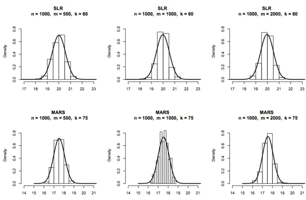
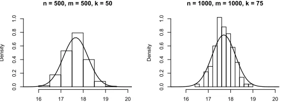
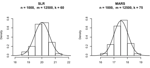
Figure 1: Histograms of subbagged predictions at x1 = 10 in the SLR case (top row) and atx1 =· · ·=x5 = 0.5 in the MARS case (bottom row). The total sample size, number of subsamples, and size of each subsample are denoted by n,m, and k, respectively in the plot titles.
5. Simulations
We present here a small simulation study in order to illustrate the limiting distributions derived in Section 2 and also to demonstrate the inference procedures proposed in the previous section. We consider two different underlying regression functions:
1. g(x1) = 2x1; X = [0,20]
2. g(x) = 10 sin(πx1x2) + 20(x3−0.05)2+ 10x4+ 5x5; X = [0,1]5
The first function corresponds to simple linear regression (SLR) and was chosen for sim-plicity and ease of visualization. The second was initially considered by Friedman (1991) in development of the Multivariate Adaptive Regression Spline (MARS) procedure and was recently investigated by Biau (2012). In each case, features were selected uniformly at
ran-dom from the feature spaces and responses were sampled fromg(x) +, whereiid∼ N(0,10), to form the training sets.
5.1 Limiting Distributions
We begin by illustrating the distributions of subbagged predictions. In the SLR case, predictions were made at x1 = 10 and in the MARS case, predictions were made atx1 =
· · · = x5 = 0.5. The histograms of subbagged predictions are shown in Figure 1. Each histogram is comprised of 250 simulations.
MARS n = 1000, m = 1000, k = 200
D
en
si
ty
15 16 17 18 19 20 21
0.0
0.1
0.2
0.3
0.4
0.5
0.6
MARS n = 1000, m = 1000, k = 1000
D
en
si
ty
16 18 20 22
0.0
0.1
0.2
0.3
0.4
0.5
0.6
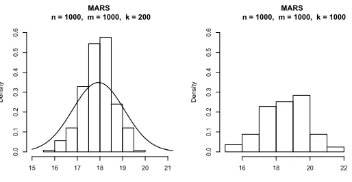
Figure 2: Histograms of subbagged predictions with larger subsample sizekand full boot-strap samples. Predictions are made atx1 =· · ·=x5 = 0.5.
rpart function in R, with the additional restriction that at least 3 observations per node
were needed in order for the algorithm to consider splitting on that node. Overlaying each histogram is the density obtained by estimating the parameters in the limiting distribution. In each case, we take the limiting distribution to be that given in result(ii) of Theorem 1; namely that the predictions are normally distributed with mean Ebn,k,m(x∗) and variance
1
α k2 mζ1,k+
1
mζk,k.
The mean Ebn,k,m(x∗) = θk was estimated as the empirical mean across the 250
sub-bagged predictions. To estimateζk,k, 5000 new subsamples of sizekwere selected and with
each subsample, a tree was built and used to predict at x1 = 10 and ˆζk,k was taken as
the empirical variance between these predictions. To estimateζ1,k, we follow the procedure
in Algorithm 3 with nz˜ = 50 and nM C = 1000 in the SLR cases and with nz˜ = 250 and nM C = 1000 in the MARS cases. Note that since we are only interested in verifying the
distributions of predictions, the variance parameters are estimated only once for each case and not for each ensemble.
It is worth noting that the same variance estimation procedure with n˜z = 250 and
nM C= 250 lead to an overestimate of the variance, so we reiterate that using a large nM C
seems to provide better results, even when nz˜ is relatively small. In each case, we use mn as a plug-in estimate for α = limmn. We also repeated this procedure and generated the distribution of predictions according to the internal variance estimation method described in Algorithm 5. Details and histograms are provided in Appendix D. These distributions appear to be the same as when the subsamples are selected uniformly at random, as in the external variance estimation method.
Note that the distributional results in Theorem 1 require lim√k
n = 0, so in practice,
-- -- ----- --- --- --- --- ---- --- -- -- -- ---- -- --- -- - --- ----- --- -- ---- -- -- --- --- -- ----- --- --- --- -- ---- -- -- ----- -- ---- -- -- --- -- -- -- --- ----- -- -- --- -- -- ---- -- --- ---- -- -- --- -- -- -
--0 50 100 150 200 250
16
20
24
Confidence Intervals for SLR Case n=200, m=200, k=30
- --- -- -- - -- -- ---- --- --- - -- ----------- -- -- -- -- --- ---- -- -- -- --- --- --- --- -- -- -------- -- --- -- --- --- -- ---- --- --- - ---- ----- -- -- --- ---- -- - --- -- ---- --- --- ----
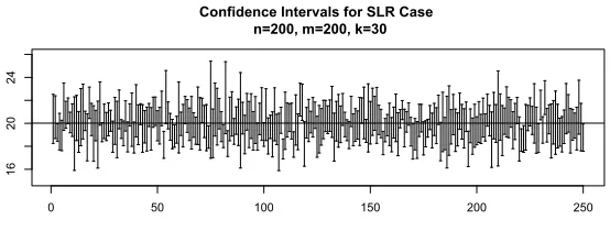
-Figure 3: Confidence Intervals for subbagged predictions.
look increasingly further from normal as kincreases. The histograms in Figure 2 show the distribution of subbagged predictions in the MARS case with n=m = 1000 and k= 200 and also with n=m =k= 1000 so that we are using full bootstrap samples to build the ensembles in the latter case. The parameters in the limiting distribution are estimated in exactly the same manner as with the smallerkfor the case wherek= 200. In the bootstrap case, we cannot follow our subbagging procedure exactly since the bootstrap samples used to build each tree in the ensemble must be taken with replacement, so we do not attempt to estimate the variance. These distributions look less normal and we begin to overestimate the variance in the case where k= 200.
5.2 Confidence Intervals
We move now to building confidence intervals for predictions and examine their coverage probabilities. We begin with the SLR case, with n = 200, m = 200, and k = 30 and as above, predict at x1 = 10. To build the confidence intervals, we generate 250 data sets and with each data set, we produce a subbagged ensemble, estimate the parameters in the limiting distribution, and take the 0.025 and 0.975 quantiles from the estimated limiting normal distribution to form an approximate 95% confidence interval. The mean of this limiting normalθk was estimated as the mean of the predictions generated by the ensemble.
The variance parameterζk,k was estimated by drawing 500 new subsamples, not necessarily
used in the ensemble, and calculating the variance between predictions generated by the resulting 500 trees andζ1,k was estimated externally usingn˜z = 50 and nM C = 250.
In order to assess the coverage probability of our confidence intervals, we first need to estimate the true mean predictionθkatx1 = 10 that would be generated by this subbagging ensemble. To estimate this true mean, we built 1000 subbagged ensembles and took the mean prediction generated by these ensembles, which we found to be 20.02 - very close to the true underlying value of 20. In this case, we found a coverage probability of 0.912, which means that 228 of our 250 confidence intervals contained our estimate of the true mean prediction. These confidence intervals are shown in Figure 3. The horizontal line in the plot is at 20.02 and represents our estimate of the true expected prediction.
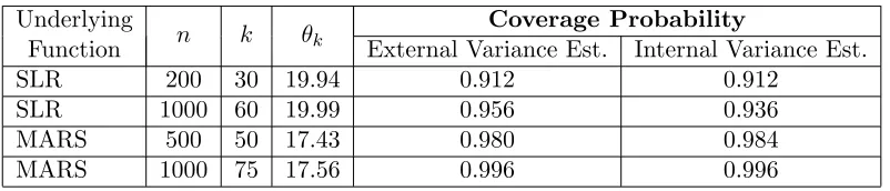
are shown in Table 1. The parameters in the limiting distributions were estimated externally in exactly the same fashion, using n˜z = 50 and nM C = 250 to estimateζ1,k. These slightly
higher coverage probabilities mean that we are overestimating the variance, which is likely due to smaller values of the estimation parametersnz˜ andnM C being used to estimateζ1,k.
Underlying
Function n k θk
Coverage Probability
External Variance Est. Internal Variance Est.
SLR 200 30 19.94 0.912 0.912
SLR 1000 60 19.99 0.956 0.936
MARS 500 50 17.43 0.980 0.984
MARS 1000 75 17.56 0.996 0.996
Table 1: Coverage probabilities
We also repeated this procedure for generating confidence intervals using the internal variance estimation method. The resulting coverage probabilities are remarkably similar to the external variance estimation method and are shown in Table 1. These ensembles were built using n˜z = 50 andnM C = 250.
5.3 Hypothesis Testing
We now explore the hypothesis testing procedure for assessing feature significance. We focus on the MARS case, where our training set now consists of 6 features X1, ..., X6, but the responseY depends only on the first 5. The values of the additional featureX6are sampled uniformly at random from the interval [0,1] and independently of the first 5 features.
We begin by looking at the distribution of test statistics when the test set consists 41 equally spaced points between 0 and 1. That is, the first test point is x1 =· · · =x6 = 0, the second is x1 = · · · = x6 = 0.025, and so on so that the last test point is x1 = · · · = x6 = 1. For this test, we are interested in looking at the difference between trees built using all features and those built using only the first 5 so that in the notation in Section 4.2, X(R) ={X
1, ..., X5}. We ran 250 simulations with n= 1000, m= 1000, and k= 75 using a test set consisting of all 41 test points, the 20 central-most points, and the 5 central-most points. The parameter Σ1,k was estimated externally usingnz˜= 100 and nM C= 5000 and
Σk,k was estimated by taking the covariance of the difference in predictions generated by
5000 trees. These covariance parameters are estimated only once instead of within each ensemble since we are only interested in the distribution of test statistics. Histograms of the resulting test statistics along with an overlay of the estimated χ2 densities are shown in the top row of Figure 4.
MARS: 5 Evenly Spaced Points
0 5 10 15
0.00
0.05
0.10
0.15
MARS: 20 Evenly Spaced Points
10 20 30 40
0.00
0.02
0.04
0.06
MARS: 41 Evenly Spaced Points
20 40 60 80 100
0.00
0.01
0.02
0.03
0.04
0.05
MARS: 5 Central Points
0 5 10 15 20 25 30
0.00
0.05
0.10
0.15
MARS: 20 Central Points
10 20 30 40 50
0.00
0.02
0.04
0.06
0.08
MARS: 41 Central Points
20 40 60 80
0.00
0.02
0.04
0.06
Figure 4: Histograms of simulated test statistics with estimatedχ2 overlay. The top row of histograms involve test points equally spaced between 0 and 1 and the bottom row corresponds to points randomly selected from the interior of the feature space.
Figure 4. Note that the bottom row appears to be a better fit and thus there appears to be some bias occuring when test points are selected near the edges of the feature space.
To check the alpha level of the test—the probability of incorrectly rejecting the null hypothesis—we simulated 250 new training sets and used the test set consisting of 41 randomly selected central points. For each training set, we built full and reduced subbagged estimates, allowed and not allowed to utilize X6 respectively, estimated the parameters, and performed the hypothesis test. For each ensemble, the variance parameter Σ1,k was
estimated externally using n˜z= 50 and nM C = 1000 and Σk,k was estimated externally on
an independently generated set of trees.
In this setup, none of the 250 simulations resulted in rejecting the null hypothesis, so our empirical alpha level was 0. A histogram of the resulting test statistics is shown on the left of Figure 5; the critical value, the 0.95 quantile of the χ2
41, is 56.942. Thus, as with the confidence intervals, we are being conservative. Recall that our confidence interval simulations with n = 1000, m = 1000, and k = 75 predicting at x = (0.5, ...,0.5) captured our true value 99.6% of the time, so this estimate of 0, though conservative, is not necessarily unexpected. We also repeated this procedure using an internal variance estimate with nz˜ = 50 and nM C = 1000 and found an alpha level of 0.14. The histogram of test
statistics resulting from the internal variance estimation method is shown on the right in Figure 5. Here we see that the correlation introduced by not taking an i.i.d. selection of subsamples to build the ensemble may be slightly inflating the test statistics.
5.4 Random Forests
External Variance Estimate
10 20 30 40 50
0.00
0.01
0.02
0.03
0.04
0.05
0.06
0.07
Internal Variance Estimate
0 20 40 60 80 100 120
0.000
0.005
0.010
0.015
0.020
0.025
Figure 5: Histograms of simulated test statistics
n = 500, m = 500, k = 50
D
en
si
ty
16 17 18 19 20
0.0
0.2
0.4
0.6
0.8
1.0
n = 1000, m = 1000, k = 75
D
en
si
ty
16 17 18 19 20
0.0
0.2
0.4
0.6
0.8
1.0
Figure 6: Histograms of random forest predictions at x1 =· · · = x5 = 0.5 with estimated normal density overlaid.
well. The histograms in Figure 6 show the distribution of predictions generated by subsam-pled random forests atx1 =· · ·=x5 = 0.5 when the true underlying function is the MARS function. These trees were grown using the randomForest function in R with the ntree
argument set to 1. At each node in each tree, 3 of the 5 featuresX1, ..., X5 were selected at random as candidates for splits and we insisted on at least 2 observations in each terminal node. The histograms show the empirical distribution of 250 subsampled random forest predictions and the overlaid density is the limiting normalN(Ern,k,m(x∗),α1k
2
mζ1,k+
1
mζk,k)
with the variance parameters estimated externally. Our estimate of the mean of this dis-tribution was taken as the empirical mean of the 250 predictions. Our estimate ofζk,k was
taken as the empirical variance of predictions across 5000 new trees and the estimate for ζ1,k was calculated withn˜z = 250 andnM C= 2000.
6. Real Data
0 10000 20000 30000 40000
JAN FEB MAR APR MAY JUN JUL AUG SEP OCT NOV DEC
Presence Absence
Figure 7: Monthly counts of Indigo Bunting observations.
on citizens, referred to as birders, to submit reports of bird observations. Location, bird species observed and not observed, effort level, and number of birds of each species observed are just a few of the variables participants are asked to provide. In addition to the data contained in these reports, landcover characteristics as reported in the 2006 United States National Land Cover Database are also available so that information about the local terrain may be used to help predict species abundance.
For our analysis, we restrict our attention to observations (and non-observations) of the Indigo Bunting species. For the first part of our analysis, we further restrict our attention to observations made during the year 2010. A little more than 400,000 reports of either presence or absence of Indigo Buntings were recorded during 2010 and the data set consists of 23 features. Like many species, the abundance of Indigo Buntings is known to fluctuate throughout the year, so we have two primary goals: (1) to produce confidence intervals for monthly abundance and (2) to show that the feature ‘month’ is significant for predicting abundance.
A presence/absence plot of Indigo Buntings by month is shown in Figure 7. A few features of this plot are worth pointing out. Most obviously, there are many more absence observations each month than presence observations. This makes sense because each time a birder submits a report, they note when Indigo Buntings are not present. Next, we see that this species is only observed during the warmer months, so month seems highly significant for predicting abundance. Finally, we see that all months have a large number of reports, so we need not worry about underreporting issues throughout the year.
- -
--
-- -
--
-External Variance Estimate Internal Variance Estimate
- -
--
-- -
--
-JAN FEB MAR APR MAY JUN JUL AUG SEP OCT NOV DEC
0.02
0.04
0.06
0.08
0.1
0.12
0.14
Ab
un
da
nce
Figure 8: Monthly confidence intervals for Indigo Bunting abundance.
the square root of the training set size. We build a total of m = 5000 trees and take the variance of these predictions at each point to be our estimates of ζk,k. We use an external
estimate with n˜z = 250 and nM C = 5000 to estimate ζ1,k. For each tree built, we require
a minimum of 20 observations to consider splitting an internal node. We also repeat this procedure using an internal estimate of variance with n˜z = 250 andnM C = 5000.
The confidence intervals are shown in Figure 8. Note that the pattern seen in Figure 7 is mirrored in the confidence interval plot: the confidence intervals are higher during months where more positive observations are recorded. It is also interesting to note that the width of the confidence intervals is larger during months of higher abundance. Observe in Figure 7 that even for months with many positive observations reported, many more negative observations are also reported. Thus, for these months there are likely a number of trees in the ensemble with nearly all positive or negative observations so we expect a higher variance in predictions. For months when very few positive observations are made, nearly all observations in the terminal node will be abscence observations, thus resulting in a very small variance and much narrower confidence intervals. Based on a visual inspection of the confidence intervals, there appears to be a clear significant difference in abundance between certain months, but we need to account for correlations in our predictions so we also conduct hypothesis tests.
We conduct these formal tests for the significance of month, following the procedure in Section 4.2. To perform this test, we randomly selected 20 points from the training set as the test set and calculated the test statistic based on an internal variance estimate with nz˜ = 250 and nM C = 5000. We calculated a test statistic of 4233.10 and a critical
test statistic of 58.02 which, though significantly smaller than the test statistic calculated on the original training set, is still significant. To ensure that the randomized months we selected did not add any accidental structure, we compared predictions generated using this training set to those generated by another training set, also with randomized months. Here we find a test statistic of only 2.36 and thus there is no significant difference between these predictions, so the trees are simply taking advantage of additional randomness. Finally, we test for a difference in predictions generated by the original training set and those generated by the training set with random values of month. In this case, we calculated a test statistic of 2336.14 which is highly significant so we can conclude that month is significant for predicting abundance and the contribution to the prediction is significantly more than would be expected by simply adding a random feature to the model.
This significant effect of month comes as no surprise as Indigo Buntings are known to be a migratory species. However, many scientists also believe that migrations may change from year to year and thus year may also be significant for predicting abundance. For this test, we used the full training data set consisting of approximately 1 million observations from 2004 to 2010 and as a test set, randomly selected 20 observations from the training set. Given this larger training set, we increased our subsample size tok= 1000 and our Monte Carlo sample size tonM C = 8000 and again performed the tests using the internel variance
estimation method. In the first setup where we test predictions from the full training set against predictions generated from the training set without year, we find a test statistic of 94.43 which means that year is significant for making predictions as it is larger than the critical value of 31.41. However, as was the case in testing the significance of month, we find that a randomly generated year feature is also significant with a test statistic of 52.51. Following in the same manner as above, we compare predictions from two training sets, each with a randomized year feature, and we find no significant difference in these predictions with a test statistic of only 4.70. Finally, we test for a difference in predictions between the full training set and a data set with random year and find that there is a significant difference in these predictions with a test statistic of 109.72. Thus, as was the case with month, we can conclude that year is significant for predicting abundance and the contribution to the prediction is significantly more than would be expected by simply adding a random feature to the model.
7. Discussion
statisti-cian’s concern for formalized inference. Our hope is that this work be seen as something of a bridge between Breiman’s two cultures.
The distributions and procedures we discuss apply to a very general class of supervised learning algorithms. We focus on bagging and random forests with tree-based base learners due to their popularity, but any supervised ensemble method that satisfies the conditions in Theorems 1 and 2 will generate predictions that have these limiting distributions and the inference procedures can be carried out in the same way. By the same reasoning, our procedures also make no restrictions on the tree-building method.
There are also some small modifications that can be made to our procedure which would still allow for an asymptotically normal limiting distribution. First, we assumed that our subsamples were selected with replacement so that in theory, the same subsample could be selected multiple times. This choice was based primarily on the fact that ensuring the exact subsample was not taken twice would typically require extra computational work. However, even for relatively small data sets, the probability of selecting the same subsample more than once is very small, and not surprisingly, the limiting distributions remain identical when the subsamples are taken without replacement. Furthermore, we also did not allow repeat observations within subsamples, which made the resulting estimator a U-statistic. Had we selected the subsamples themselves with replacement, our estimator would be a V-statistic—a closely related class of estimators introduced by von Mises (1947)—and similar theory could be developed. It is also worth pointing out that in practice, we always selected the same number of subsamplesmnand subsample sizekn for each prediction pointx∗ but
in theory, these could be chosen differently for each point of interest and the same can be said of the estimation parametersnz˜ and nM C. However, choosing different values of these
parameters for different prediction points involves significantly more bookkeeping and we advise against it in practice.
Our approach also raises some issues. Perhaps most obviously, the parameter in our inference procedures is the expected prediction generated by trees built in the prescribed fashion, as opposed to the true value of the underlying regression function,F(x∗). Though some tree-building methods have been shown to be consistent, the bias introduced may not be negligible so we have to be careful about interpreting our results. It may be possible to employ a residual bootstrap to try and correct for bias and we plan to explore this in future work. Another open question that we hope to address in future work is how to select the test points when testing feature significance. In the eBird application, we randomly selected points from the training set, but it would be beneficial to investigate optimal strategies for selecting both the number and location of test points. Finally, the distributional results we provide could potentially allow us to test more complex hypotheses about the structure of the underlying regression function, for example, the interaction between covariates.
Acknowledgments
Appendix A.
We present here the proofs of the theorems provided in Section 2. We begin with a lemma from Lee (1990).
Lemma 3 (Lee 1990, Lemma A, page 201) Leta1, a2, ...be a sequence of constants such that limn→∞ n1Pni=1ai = 0andlimn→∞ n1Pni=1a2i =σ2 and let the random variablesM1, ..., Mn
have a multinomial distribution, multinomial(mn;m1n, ...,m1n). Then as mn, n → ∞, the
limiting distribution of
m−1n /2
n
X
i=1
ai(Mi−mn/n)
is N(0, σ2).
Additionally, it will be useful to have the limiting distribution of complete infinite order U-statistics, which we provide in the lemma below.
Lemma 4 Let Z1, Z2, ...iid∼ FZ and let Un,kn be a complete, infinite order U-statistic with
kernelhkn satisfying Condition 1 andθkn =Ehkn(Z1, ..., Zkn) such thatEh
2
kn(Z1, ..., Zkn)≤
C <∞ for alln and some constant C andlim√kn
n = 0. Then
√
n(Un,kn−θkn)
p k2
nζ1,kn
d
→ N(0,1).
The proof of Lemma 3 is provided in Lee (1990) page 201. The proof of Lemma 4 follows in exactly the same fashion as the proof of result(i) in Theorem 1 below. We take advantage of these lemmas in the following proofs.
Theorem 1 Let Z1, Z2, ... iid∼ FZ and let Un,kn,mn be an incomplete, infinite order
U-statistic with kernel hkn that satisfies Condition 1. Let θkn = Ehkn(Z1, ..., Zkn) such that
Eh2kn(Z1, ..., Zkn) ≤ C < ∞ for all n and some constant C, and let lim
n
mn = α. Then as
long as lim√kn
n = 0 and limζ1,kn 6= 0,
(i) ifα= 0, then
√
n(U√n,kn,mn−θkn)
k2
nζ1,kn
d
→ N(0,1).
(ii) if0< α <∞, then
√
mn(Un,kn,mn−θkn)
q
k2n
αζ1,kn+ζkn,kn
d
→ N(0,1).
(iii) ifα=∞, then
√
mn(U√n,kn,mn−θkn)
ζkn,kn
d
Proof:
(i) Suppose first that α= 0. In the interest of clarity, we follow the H´ajek projection method discussed in Van der Vaart (2000) chapters 11 and 12. Define the H´ajek projection of Un,kn,mn−θkn as
ˆ
Un,kn,mn =
n
X
i=1
E(Un,kn,mn−θkn |Zi)−(n−1)E(Un,kn,mn−θkn)
=
n
X
i=1
E(Un,kn,mn−θkn |Zi)
so that for each term in the sum, we have
E(Un,kn,mn−θkn |Zi) =E
1 mn
X
β
hkn(Zβ1, ..., Zβkn)−θkn
Zi
= 1 mn
X
β
E hkn(Zβ1, ..., Zβkn)−θkn
Zi
(7)
where, in keeping with the notation in Van der Vaart (2000), we letβ index the subsamples. Define h1,kn(x) = Ehkn(x, Z2, ..., Zkn)−θkn and let W be the number of subsamples that
contain i. Since we assume that the subsamples are selected uniformly at random with replacement,
W ∼Binom mn, n−1
kn−1
n k
!
so we can rewrite (7) as
1 mn
X
β
E
E(hkn(Zβ1, ..., Zβkn)−θkn|Zi)
W
= 1 mnE
(W h1,kn(Zi))
= 1 mn
mn
n−1
kn−1
n k
!
h1,kn(Zi)
!
= kn
nh1,kn(Zi)
so that taking the sum yields
ˆ
Un,kn,mn =
kn
n
n
X
i=1
Now we establish the asymptotic normality of ˆUn,kn,mn. Define the triangular array
kn1h1,kn1(Z1), . . . , kn1h1,kn1(Zn1)
kn1+1h1,kn1+1(Z1), . . . , kn1+1h1,kn1+1(Zn1+1)
. .
. .
. .
kn1+jh1,kn1+j(Z1), . . . , kn1+jh1,kn1+j(Zn1+j)
so that for each variable in the array, we have
E(knh1,kn(Zi)) =kn(θkn−θkn) = 0
and
var(knh1,kn(Zi)) =k
2
nvar(h1,kn(Zi)) =k
2
nζ1,kn
and thus the row-wise sum of the variances is
s2n=
n
X
i=1
var(knh1,kn(Zi)) =nk
2
nζ1,kn.
Forδ >0, the Lindeberg condition is given by
lim
n→∞
n
X
i=1 1 nk2
nζ1,kn
Z
|knh1,kn(Zi)|≥δkn √
nζ1,kn
k2nh21,kn(Zi)dP
= lim
n→∞
n
X
i=1 1 nζ1,kn
Z
|h1,kn(Zi)|≥δ √
nζ1,kn
h21,kn(Zi)dP
≤ lim
n→∞1≤maxi≤n
1 ζ1,kn
Z
|h1,kn(Zi)|≥δ √
nζ1,kn
h21,kn(Zi)dP
= lim
n→∞ 1 ζ1,kn
Z
|h1,kn(Z1)|≥δ
√
nζ1,kn
h21,kn(Z1)dP (8) = 0
by Condition 1, and thus the Lindeberg condition is satisfied. Thus, by the Lindeberg-Feller central limit theorem,
P
jknh1,kn(Zj)
sn
d
→ N(0,1)
or, rewriting,
√
nUˆn,kn,mn
p k2
nζ1,kn
d
Now, we need to compare the limiting variance ratio of Un,kn,mn and its H´ajek projection
ˆ
Un,kn,mn. For incomplete U-statistics of fixed rank, Blom (1976) showed that the variance
of the incomplete U-statisticUm consisting ofm subsamples selected uniformly at random
with replacement is given by
ζk
mn
+
1− 1
mn
var(U)
whereU is the complete U-statistic analogue. Extending this result to our situation where kand m may both depend on n, we have
var(Un,kn,mn) =
ζkn,kn
mn
+
1− 1
mn
var(Un,kn)
where the variance of the complete U-statisticUn,kn is given by
kn
X
c=1
kn!2
c!(kn−c)!2
(n−kn)(n−kn−1)· · ·(n−2kn+c+ 1)
n(n−1)· · ·(n−kn+ 1)
ζc,kn.
The details of this calculation are described in Van der Vaart (2000) page 163. Thus, looking at the limit of the variance ratio, we have
lim
n→∞
var(Un,kn,mn)
var( ˆUn,kn,mn)
! = lim n→∞ ζkn,kn
mn +
1−m1
n
var(Un,kn)
k2
n
nζ1,kn
= lim
n→∞
n ζkn,kn
mnk2nζ1,kn
+ lim
n→∞
1− 1
mn
lim
n→∞
n var(Un,kn)
k2
nζ1,kn
= 0 + lim
n→∞
n var(Un,kn)
k2
nζ1,kn
= lim
n→∞
Pkn
c=1
kn!2
c!(kn−c)!2
(n−kn)(n−kn−1)···(n−2kn+c+1)
(n−1)···(n−kn+1) ζc,kn
k2
nζ1,kn
= lim n→∞
kn!2
(kn−1)!2
(n−kn)(n−kn−1)···(n−2kn+2)
(n−1)···(n−kn+1) ζ1,kn
k2
nζ1,kn
= lim
n→∞
(n−kn)(n−kn−1)· · ·(n−2kn+ 2)
(n−1)· · ·(n−kn+ 1)
= 1.
Note that in the second line, lim n ζkn,kn
mnk2nζ1,kn
= 0 since mn
n →0,ζ1,kn 90 by assumption,
and ζkn,kn 9 ∞ since Eh
2
kn(Z1, ..., Zkn) is bounded. Finally, by Slutsky’s Theorem and
Theorem 11.2 in Van der Vaart (2000), we have
√
n(Un,kn,mn −θkn)
p k2
nζ1,kn
=
√
n(Un,kn,mn−θkn−Uˆn,kn,mn+ ˆUn,kn,mn)
p k2
=
√
n(Un,kn,mn−θkn−Uˆn,kn,mn)
p k2
nζ1,kn
+
√
nUˆn,kn,mn
p k2
nζ1,kn
where√n(Un,kn,mn−θkn−Uˆn,kn,mn)/
p k2
nζ1,kn
P
→0 and
√
nUˆn,kn,mn
p k2
nζ1,kn
d
→ N(0,1)
so that
√
n(Un,kn,mn−θkn)
p k2
nζ1,kn
d
→ N(0,1)
as desired.
(ii) &(iii) Now suppose α >0. We follow the proof technique in Lee (1990) page 200 which is based on the work of Janson (1984). Let S(n,kn) = {Si : i = 1, ..., knn
} denote the set of all possible subsamples of size kn. In the following work, we use the notation
(n, kn) in place of knn
in subscripts and summation notation. Consider the random vector Mn,kn = (MS1, ..., MS(n,kn)), where the i
th element denotes the number of times the ith
subsample appears inUn,kn,mn. Since the subsamples are selected uniformly at random with
replacement, Mn,kn ∼ multinomial(mn;
1 (n kn)
, ..., 1 (n kn)
). Let φn,kn,mn be the characteristic
function of √mn(Un,kn,mn −θkn) and let φ denote the limiting characteristic function of √
n(Un,kn −θkn) where Un,kn is the corresponding complete U-statistic. Additionally, let
φ(n,kM)
n,mn be the characteristic function of the random variable
m−1n /2 (n,k)
X
i=1
MSi−
mn n kn
hkn(Si)−θkn
Z1, ..., Zn. Then we have
φn,kn,mn(t) =E(exp[it √
mn(Un,kn,mn−θkn)])
=E
exp
itm−1n /2
(n,kn)
X
i=1
MSi(hkn(Si)−θkn)
=E E exp
itm−1n /2
(n,kn)
X
i=1
MSi(hkn(Si)−θkn)
Z1, ..., Zn
=E E exp "
itm−1n /2
(n,kn)
X
i=1
MSi+
mn n kn − mn n kn
× hkn(Si)−θkn
!#
Z1, ..., Zn