On Binary Embedding using Circulant Matrices
Felix X. Yu1 [email protected]
Aditya Bhaskara2 [email protected]
Sanjiv Kumar1 [email protected]
Yunchao Gong3 [email protected]
Shih-Fu Chang4 [email protected]
1
Google Research, New York, NY 10011
2
University of Utah, Salt Lake City, UT 84112
3
Snap, Inc., Venice, CA 90291
4
Columbia University, New York, NY 10027
Editor:Mikhail Belkin
Abstract
Binary embeddings provide efficient and powerful ways to perform operations on large scale data. However binary embedding typically requires long codes in order to preserve the discriminative power of the input space. Thus binary coding methods traditionally suffer from high computation and storage costs in such a scenario. To address this problem, we propose Circulant Binary Embedding (CBE) which generates binary codes by projecting the data with a circulant matrix. The circulant structure allows us to use Fast Fourier Transform algorithms to speed up the computation. For obtainingk-bit binary codes from d-dimensional data, our method improves the time complexity fromO(dk) toO(dlogd), and the space complexity fromO(dk) toO(d).
We study two settings, which differ in the way we choose the parameters of the circulant matrix. In the first, the parameters are chosen randomly and in the second, the parameters are learned using the data. For randomized CBE, we give a theoretical analysis comparing it with binary embedding using an unstructured random projection matrix. The challenge here is to show that the dependencies in the entries of the circulant matrix do not lead to a loss in performance. In the second setting, we design a novel time-frequency alternating optimization to learn data-dependent circulant projections, which alternatively minimizes the objective in original and Fourier domains. In both the settings, we show by extensive experiments that the CBE approach gives much better performance than the state-of-the-art approaches if we fix a running time, and provides much faster computation with negligible performance degradation if we fix the number of bits in the embedding.
Keywords: structured matrix, circulant matrix, dimensionality reduction, binary em-bedding, FFT
1. Introduction
Sketching and dimensionality reduction have become powerful and ubiquitous tools in the analysis of large high-dimensional data sets, with applications ranging from computer vision, to biology, to finance. The celebrated Johnson-Lindenstrauss lemma says that
pro-c
jecting high dimensional points to a random O(logN)-dimensional space approximately preserves all the pairwise distances between a set ofN points, making it a powerful tool for nearest neighbor search, clustering, etc. This started the paradigm of designing low dimen-sional sketches (or embeddings) of high dimensional data that can be used for efficiently solving various information retrieval problems.
More recently, binary embeddings (or embeddings into {0,1}k or {−1,1}k) have been
developed for problems in which we care about preserving the angles between high di-mensional vectors (Li et al., 2011; Gong et al., 2013; Raginsky and Lazebnik, 2009; Gong et al., 2012b; Liu et al., 2011). The main appeal of binary embeddings stems from the fact that storing them is often much more efficient than storing real valued embeddings. Furthermore, operations such as computing the Hamming distance in binary space can be performed very efficiently either using table lookup, or hardware-implemented instructions on modern computer architectures.
In this paper, we study binary embeddings of high-dimensional data. Our goal is to address one of its main challenges: even though binary embeddings are easy to manipulate, it has been observed that obtaining high accuracy results requires the embeddings to be rather long when the data is high dimensional (Li et al., 2011; Gong et al., 2013; S´anchez and Perronnin, 2011). Thus in applications like computer vision, biology and finance (where high dimensional data is common), the task of computing the embedding is a bottleneck. The natural algorithms have time and space complexity O(dk) per input point in order to produce ak-bit embedding from ad-dimensional input. Our main contribution in this work is to improve these complexities to O(dlogd) for time andO(d) for space complexity.
Our results can be viewed as binary analogs of the recent work on fast Johnson-Lindenstrauss transform. Starting with the work of Ailon and Chazelle (Ailon and Chazelle, 2006), there has been a lot of beautiful work on fast algorithms for dimension reduction with the goal of preserving pairwise distances between points. Various aspects, such as exploiting sparsity, and using structured matrices to reduce the space and time complexity of dimension reduction, have been explored (Ailon and Chazelle, 2006; Matouˇsek, 2008; Liberty et al., 2008). But the key difference in our setting is that binary embeddings are
non-linear. This makes the analysis tricky when the projection matrices do not have
in-dependent entries. Binary embeddings are also better suited to approximate the angles between vectors (as opposed to distances). Let us see why.
The general way to compute a binary embedding of a data point x∈Rdis to first apply
a linear transformation Ax (for a k×d matrix A), and then apply a binarization step. We consider the natural binarization of taking the sign. Thus, for a point x, the binary embedding into {−1,1}dwe consider is
h(x) = sign(Ax), (1)
where A ∈ Rk×d as above, and sign(·) is a binary map which returns element-wise sign1.
How should one pick the matrixA? One natural choice, in light of the Johnson-Lindenstrauss lemma, is to pick it randomly, i.e., each entry is sampled from an independent Gaussian.
This data oblivious choice is well studied (Charikar, 2002; Raginsky and Lazebnik, 2009),
and has the nice property that for two data vectors x,y, the `1 distance between their
embeddings is proportional to the angle betweenx andy, in expectation (over the random entries in A). This is a consequence of the fact that for anyx,y∈Rd, if r is drawn from
N(0,1)d,
Pr[signhx,ri= signhy,ri] = ∠(x,y)
π . (2)
Other data oblivious methods have also been studied in the literature, by choosing dif-ferent distributions for the entries ofA. While these methods do reasonably well in practice, the natural question is if adapting the matrix to the data allows us to use shorter codes (i.e., have a smaller k) while achieving a similar error. A number of such data-dependent tech-niques have been proposed with different optimization criteria such as reconstruction error (Kulis and Darrell, 2009), data dissimilarity (Norouzi and Fleet, 2012; Weiss et al., 2008), ranking loss (Norouzi et al., 2012), quantization error after PCA (Gong et al., 2012a), and pairwise misclassification (Wang et al., 2010). As long as data is relatively low dimensional, these methods have been shown to be quite effective for learning compact codes.
However, theO(kd) barrier on the space and time complexity barrier prevents them from being applied with very high-dimensional data. For instance, to generate 10K-bit binary codes for data with 1M dimensions, a huge projection matrix will be required needing tens of GB of memory.2
In order to overcome these computational challenges, Gong et al. (2013) proposed a
bilinear projectionbased coding method. The main idea here is to reshape the input vector
xinto a matrixZ, and apply a bilinear projection to get the binary code:
h(x) = sign(RT1ZR2). (3)
When the shapes of Z,R1,R2 are chosen appropriately3, the method has time and space
complexitiesO(d√k) andO(√dk) respectively. Bilinear codes make it feasible to work with data sets of very high dimensionality and have shown good results for a variety of tasks.
1.1 Our results
In this work, we propose a novel technique, called Circulant Binary Embedding (CBE), which is even faster than the bilinear coding. The main idea is to impose a circulant
(described in detail in Section 3) structure on the projection matrixA in (1). This special structure allows us to compute the product Ax in time O(dlogd) using the Fast Fourier Transform (FFT), a tool of great significance in signal processing. The space complexity is also just O(d), making it efficient even for very high dimensional data. Table 1 compares the time and space complexity for the various methods outlined above.
Given the efficiency of computing the CBE, two natural questions arise: how good is the obtained embedding for various information retrieval tasks? and how should we pick the parameters of the circulant A?
In Section 4, we study the first question forrandomCBE, i.e., when the parameters of the circulant are picked randomly (independent Gaussian, followed by its shifts). Specifically,
2. In the oblivious case, one can generate the random entries of the matrix on-the-fly (with fixed seeds) without needing to store the matrix, but this increases the computational time even further.
3. Specifically,Z∈R
√
d×√d
,R1,R2∈R
√
k×√d
Method Time Space Time (optimization) Unstructured O(dk) O(dk) O(N d2k)
Bilinear O(d√k) O(√dk) O(N d√k) Circulant (k≤d) O(dlogd) O(d) O(N dlogd) Circulant (k > d) O(klogd) O(k) O(N klogd)
Table 1: Comparison of the time and space complexities. dis the input dimensionality, and
kis the output dimensionality (number of bits). N is the number of instances used for learning data-dependent projection matrices. See Section 3.3 for discussions on k < dand k > d.
we analyze theangle estimatingproperty of binary embeddings (Eq.(1)), which is the basis for its use in applications. Under mild assumptions, we show that using a random circulant
Ahas the same qualitative guarantees as using fully randomA. These results provide some of the few theoretical guarantees we are aware of, for non-linear circulant-based embeddings. We defer the formal statements of our results to Section 4, Theorems 3 and 4. We note that in independent and very recent work, Choromanska et al. (Choromanska et al., 2016) obtain a qualitatively similar analysis of CBE, however the bounds are incomparable to ours.
In Section 5, we study the second question, i.e., learning data-dependent circulant matri-ces. We propose a novel and efficient algorithm, which alternatively optimizes the objective in the original and frequency domains.
Finally in Section 7, we study the empirical performance of circulant embeddings via extensive experimentation. Compared to the state-of-the-art, our methods improve the performance dramatically for a fixed computation time. If we instead fix the number of bits in the embedding, we observe that the performance degradation is negligible, while speeding up the computation many-fold (see Section 7).
2. Background and related work
The lemma of Johnson and Lindenstrauss (Johnson and Lindenstrauss, 1984) is a fun-damental tool in the area of sketching and dimension reduction. The lemma states that if we have N points in d-dimensional space, projecting them to an O(logN) dimensional space (independent ofd!) preserves all pairwise distances. One way of doing the projection is by a random Gaussian matrix. Formally,
Lemma 1 (Johnson Lindenstrass lemma) Let S be a set of N points in Rd. Let A∈
Rk×dbe a matrix whose entries are drawn i.i.d from N(0,1). Then with probability at least
1−2N2e−(2−3)k/4
(1−)kx−yk2≤
1
√
kkA(x−y)k2 ≤(1 +)kx−yk2 (4)
Whenk=O(logN/2), the probability above can be made arbitrarily close to 1. The result has also been shown to be optimal even if the projection can be chosen data-dependently (Larsen and Nelson, 2016). Due to the simplicity and theoretical support, random pro-jection based dimensionality reduction has been applied in broad applications including approximate nearest neighbor research (Indyk and Motwani, 1998), dimensionality reduc-tion in databases (Achlioptas, 2003), and bi-Lipschitz embeddings of graphs into normed spaces (Frankl and Maehara, 1988).
However a serious concern in a few applications is the dependence of kon the accuracy (O(1/2)). The space and time complexity of dimension reduction areO(kd), if the compu-tation is done in the natural way. Are there faster methods whenkis reasonably large? As mentioned earlier, the line of work starting with (Ailon and Chazelle, 2006) aims to improve the time and space complexity of dimension reduction. This led to work showing Johnson-Lindenstruss-type guarantees with structured matrices (with some randomness), including Hadamard matrices along with a sparse random Gaussian matrix (Ailon and Chazelle, 2006), sparse matrices (Matouˇsek, 2008), and Lean Walsh Transformations (Liberty et al., 2008). The advantage of using structured matrices is that the space and computation cost can be dramatically reduced, yet the distance preserving property remains to be competitive.
In this context, randomized circulant matrices (which are also the main tool in our work) have been studied, starting with the works (Hinrichs and Vyb´ıral, 2011; Vyb´ıral, 2011). The dimension reduction comprises of random sign flips followed by multiplication by a randomized circulant matrix. For d-dimensional input, reducing the dimension to k
for k < d has time complexity O(dlogd) and space complexity O(d), independent of k. Proving bounds similar to Lemma 1 turns out to be much more challenging because the entries of the projection matrix are now highly dependent, and thus concentration bounds are hard to prove. The first analysis (Hinrichs and Vyb´ıral, 2011) showed that reducing toO(log3N/2) dimensions (compared toO(logN/2) in Lemma 1) preserves all pairwise distances with high probability. This was improved toO(log2N/2) in (Vyb´ıral, 2011), and furthermore toO(log(1+δ)N/2) in (Zhang and Cheng, 2013), using matrix-valued Bernstein inequalities. These works provide the motivation for our theoretical results, however the key difference for us is the binarization step, which is highly non-linear. Thus we need to develop new machinery for our analysis.
Binary embeddings. Recently, structured matrices used in the context of the fast JL
transform (a combination of Hadamard and sparse random Gaussian matrices) have also been studied for binary embedding (Dasgupta et al., 2011), and more recently (Yi et al., 2015). In particular, Yi et al. (2015) showed that the method can achieve distance pre-serving error with O(logN/2) bits and O(dlogd) computational complexity, for N points (N √d). In this work, we study the application of using the circulant matrix for bi-nary embedding. The work extends and provides theoretical justification for our previous conference paper on this topic (Yu et al., 2014).
3. Circulant Binary Embedding
Let us start by describing our framework and setting up the notation that we use in the rest of the paper.
3.1 The Framework
We will now describe our algorithm for generatingk-bit binary codes fromd-dimensional real vectors. We start by discussing the case k = d and move to the general case in Section 3.3. The key player is the circulant matrix, which is defined by a real vector
r= (r0, r1,· · · , rd−1)T (Gray, 2006).
Cr:=
r0 rd−1 . . . r2 r1 r1 r0 rd−1 r2
..
. r1 r0 . .. ...
rd−2 . .. ... rd−1 rd−1 rd−2 . . . r1 r0
. (5)
Let D be a diagonal matrix with each diagonal entry σi, i = 0,· · ·, d−1, being a
Rademacher variable (±1 with probability 1/2):
D=
σ0 σ1
σ2
. ..
σd−1
. (6)
Forx∈Rd, its d-bit Circulant Binary Embedding (CBE) withr∈
Rd is defined as:
h(x) = sign(CrDx), (7)
whereCr is defined as above. Note that applyingD toxis equivalent to applying a random sign flip to each coordinate of x. The necessity of such an operation is discussed in the introduction of Section 4. Since sign flipping can be carried out as a preprocessing step for each input x, here onwards for simplicity we will drop explicit mention of D. Hence the binary code is given ash(x) = sign(Crx).
3.2 Computational Complexity
The main advantage of a circulant based embedding is that it can be computed quickly using the Fast Fourier Transform (FFT). The following is a folklore result, whose proof we include for completeness.
Proposition 2 For a d-dimensional vectorxand anyr∈ <d, thed-bit CBEsign(C
r(Dx))
can be computed using O(d) space andO(dlogd) time.
Proof The space complexity comes only from the storage of the vectorr and the signsD
The main property of a circulant matrix is that for any vectory∈Rd, we can compute
Cry in timeO(dlogd). This is because
Cr=Fd−1 diag(Fdr) Fd, (8)
whereFdis the matrix corresponding to the Discrete Fourier Transform (DFT) of periodicity
N, i.e., whose (i, j)th entry is given by
Fd(i, j) =ωij, (9)
where ω is the Nth root of unity e−2πι/N. The celebrated Fast Fourier Transform algo-rithm (Oppenheim et al., 1999) says that for anyz ∈Rd, we can compute Fdz and Fd−1z
in time O(dlogd), using O(d) space. This immediately implies that we can compute Cry within the same space and time complexity bounds.
3.3 Generalizing to k6=d
The computation above assumed that number of bits we produce (k) is equal to the input dimension. Let us now consider the general case.
When k < d, we still use the circulant matrix R ∈ Rd×d with d parameters, but the
output is set to be the first kelements in (7). This is equivalent to the operation
Φ(x) := sign(Cr,kDx), (10)
whereCr,k the so-called partial circulant matrix, which is Cr truncated to krows. We note that CBE with k < d is not computationally more efficient than that withk=d.
Whenk > d, using a singlercauses repetition of bits, so we propose usingCrfor multiple
r, and concatenating their output. This gives the computational complexityO(klogd), and space complexity O(k). Note that as the focus of this paper is on binary embedding on high-dimensional data, from here onwards, we assume k≤ d. The k > d case is useful in other applications such as neural network (Cheng et al., 2015) and kernel approximation (Yu et al., 2015).
3.4 Choosing the Parameters r
We have presented the general framework as well as its space and computation efficiency in this section. One critical question left unanswered is how to decide the parameter r. As mentioned in the introduction, we consider two solutions. In Section 4, we study the randomized version, where each element ofris independently sampled from a unit Gaussian distribution. This is inspired by the popular Locality Sensitive Hashing (simhash) approach. Section 5 introduces an optimized version, where the parameters are optimized based on training data and an distance preserving objective function.
4. Randomized CBE – A Theoretical Analysis
matrixCr,k, forr∼ N(0,1)d. The embedding we consider for an x∈Rd is given by
Φ(x) := sign(Cr,kDx). (11)
As before,Dis a diagonal matrix of signs. Hence the embedding uses 2dindependent ‘units’ of randomness.
Now, for any two vectors x,y∈Rd, we have that
E
1
2kkΦ(x)−Φ(y)k1
= ∠(x,y)
π , (12)
implying that the random variable (1/2k)kΦ(x)−Φ(y)k1 provides an estimate for θ/π, whereθ:=∠(x,y).
We present two main results. In the first, we bound the variance of the above angle estimate for given x,y. We compare with the variance in the fully independent case, i.e., when we consider the embedding sign(Ax), whereAis ak×dmatrix with all entries being independent (and unit normal). In this case, the variance of the estimator in Eq. (12) is equal to 1kπθ 1− θ
π
.4
We show that using a circulant matrix instead of A above has a similar dependence on
k, as long as the vectors are well spread. Formally,
Theorem 3 Let x,y∈Rd, such that max{kxk
∞/kxk2,kyk∞/kyk2} ≤ρ, for some
param-eter ρ < 1, and set θ = ∠(x,y). The variance of the averaged hamming distance of k-bit code generated by randomized CBE is
var
1
2kkΦx−Φyk1
≤ 1
k θ π
1− θ
π
+ 32ρ. (13)
The variance above is over the choice of rand the random signs D.
Remark. For typical vectors inRd, we havekxk∞/kxk2 to be O(logd/
√
d). Further, by using the idea from Ailon and Chazelle (Ailon and Chazelle, 2006), we can pre-process the data by multiplying it with a randomly signed Hadamard matrix, and guarantee such an
`∞ bound with high probability.5 Therefore the second term becomes negligible for large d. The above result suggests that the angle preservation performance of CBE (in term of the variance) is as good as LSH for high-dimensional data.
Our second theorem gives a large-deviation bound for the angle estimate, also assuming that the vectors are well-spread. This will then enable us to obtain a dimension reduction theorem which preserves all angles up to an additive error.
Theorem 4 Letx,y∈Rdwith∠(x,y) =θ, and supposemax{kxk
∞/kxk2,kyk∞/kxk2} ≤
ρ, for some parameter ρ. Now consider the k-dimensional CBE Φx,Φy of x,y respectively,
for some k < d. Suppose ρ≤ 16klog(θ2k/δ). For any δ >0, we have:
Pr
1
2kkΦx−Φyk1− θ π
> 4 log(√k/δ)
k
< δ. (14)
4. We are computing the variance of an average of i.i.d. Bernoulli random variables which take value 1
with probabilityp=θ/π.
5. However, applying this pre-processing leads todensevectors, which may be memory intensive for some
applications. In this case, dividing the co-ordinates into blocks of size ∼ k2 and performing the
Qualitatively, the condition on ρ is similar to the one we implicitly have in Theorem 3. Unless ρ=o 1kθπ(1− θπ), the additive term dominates, so for the bound to be interesting, we need this condition on ρ.
We observe that Theorem 4 implies a Johnson-Lindenstrauss type theorem.
Corollary 5 Suppose we have N vectors u0,u1, . . . ,uN−1 in Rd, and define
ρij = max{kuik∞/kuik2,kujk∞/kujk2}, θij =∠(ui,uj). (15) Let >0 be a given accuracy parameter and let k=Clog2n/2. Then for all i, j such that ρij <
θ2
ij
16klog(2kN2), we have
1
2kkΦi−Φjk1− θij
π
< , (16)
with probability at least 3/4.
Proof We can set δ = 1/2N2 in Theorem 4 and then take a union bound over all N2
choices of pairsi, jto obtain a failure probability≤1/4. Further, for our choice ofk, setting
C= 144 and assuming N is large enough thatk < N, we have
4 log(k/)
√
k <
12δlogN
√
C·logN < . (17)
In the remainder of the section, we will prove the above theorems. We start with Theorem 3, whose proof will give a basic framework for that of Theorem 4.
4.1 Variance of the angle estimator
For a vector x and an index i, we denote by s→i(x) the vector shifted by i positions:
thejth entry ofs→i is the ((j−i)modd)’th entry of x. Further, let us define
Fi =
1−sign(s→i(r)TDx) sign(s→i(r)TDy)
2 −
θ
π. (18)
where s→i(·) is defined as the operator circularly shifting a vector by i elements6. By
definition, we have
var
1
2kkΦx−Φyk1
=var
"
1
k
k
X
i=1
Fi
#
. (19)
6. The above comes with a slight abuse of notation, where the first column (instead of row) of the projection
Without loss of generality, we assume kxk2,kyk2= 1 (since we only care about the angle). The mean of each Fi is zero, and thusE[k1Pki=1Fi] = 0. Thus the variance is equal to
var
"
1
k
k−1
X i=0 Fi # =E 1 k2
k−1
X
i=0
Fi
!2
(20)
=E
" Pk−1
i=0 Fi2+
P
i6=jFiFj
k2
#
= 1
k2
k·EF12+
X
i6=j
E(FiFj)
= 1 k θ π
1− θ
π
+ 1
k2
X
i6=j
E(FiFj). (21)
The last step is based on variance of the fully independent case: the variance of a Bernoulli random variable which takes value 1 with probabilityp=θ/π is πθ 1−θ
π
.
To prove the theorem, it suffices to show that E(FiFj)≤32ρ for alli6=j. Without loss
of generality, we can assume thati= 0, and considerE(F0Fj). By definition, it is equal to
E
1−sign(rTDx) sign(rTDy)
2 −
θ π
1−sign(s→j(r)TDx) sign(s→j(r)TDy)
2 −
θ π
.
The trick now is to observe that
s→j(r)Tx=rTs→(d−j)(x). (22)
Thus settingt=d−j, we can write the above as
E
1−sign(rTDx) sign(rTDy)
2 −
θ π
1−sign(rTs
→t(Dx)) sign(rTs→t(Dy))
2 −
θ π
.
The key idea is that we expect the vectors→t(Dx) to be nearly orthogonal to the space
containing Dx,Dy. This is because D is a diagonal matrix of random signs, and x and y
are vectors with small`∞ norm. We show this formally in Lemma 7.
Why does this help? Suppose for a moment that u :=s→t(Dx) and v:=s→t(Dy) are
both orthogonal to span{Dx,Dy}. Then for a random Gaussian r, the random variables sign(rTu) sign(rTv) and sign(rTDx) sign(rTDy) are independent, because the former de-pends only on the projection of r onto span{u,v}, while the latter depends only on the projection ofronto span{Dx,Dy}. Now if these two spaces are orthogonal, the projections of a Gaussian vector onto these spaces are independent (this is a fundamental property of multidimensional Gaussians). This implies that the expectation of the product above is equal to the product of the expectations, which is zero (each expectation is zero).
The key lemma (see below) now says that even if u and v as defined above are nearly
Lemma 6 Let a,b,u,v be unit vectors in Rd such that ∠(a,b) =∠(u,v) = θ, and let Π
be the projector onto span{a,b}. Suppose max{kΠuk,kΠvk}=δ <1. Then we have
E
1−sign(rTa) sign(rTb)
2 −
θ π
1−sign(rTu) sign(rTv)
2 −
θ π
≤2δ. (23)
Here, the expectation is over the choice ofr.
The proof of the above lemma is moved to Appendix A.1.
We use the lemma with a =Dx and b =Dy. To show Theorem 3, we have to prove that
E[max{kΠuk,kΠvk}]≤16ρ, (24)
where Π,u,vare defined as in the statement of Lemma 6. The expectation now is over the choice ofD. This leads us to our next lemma.
Lemma 7 Letp,q∈Rdbe vectors that satisfykpk
2 = 1andkqk∞< ρfor some parameter
ρ, and suppose D := diag(σ0, σ1, . . . , σd−1), where σi are random ±1 signs. Then for any
0< t < d, we have
Pr[hDp, s→t(Dq)i> γ]≤e−γ
2/8ρ2
. (25)
Note that the probability is over the choice of D.
The proof of the above lemma is moved to Appendix A.2. We remark that the lemma only assumes thatp is a unit vector, it need not have a small `∞ norm.
We can now complete the proof of our theorem. As noted above, we need to show (24). To recall, Π is the projector onto span{Dx,Dy}, and we need to bound:
E[max{kΠuk,kΠvk}]≤E[kΠuk] +E[kΠvk]. (26)
Letx,z be an orthonormal basis for span{x,y}; then it is easy to see that for any diagonal
D with ±1 entries on the diagonal, Dx,Dz is an orthonormal basis for span{Dx,Dy}. Thus
E[kΠuk]≤E[|hu,Dxi|+|hu,Dzi|]. (27)
Now by Lemma 7,
Pr[|hu,Dxi|> tρ]≤e−t2/4. (28) Integrating over t, we get E[|hu,Dxi|]≤4ρ. Thus we can bound the LHS of (26) by 16ρ,
completing the proof of the theorem.
4.2 The Johnson-Lindenstrauss Type Result
Next, we turn to the proof of Theorem 4, where we wish to obtain a strong tail bound. At a high level, the argument consists of two steps:
• First, show that with probability 1− over the choice of D, the k translates of x,y
satisfy certain orthogonality properties (this is in the same spirit as Lemma 7).
Next will will show the two steps respectively. Throughout this section, we denote by
X0, X1, . . . , Xk−1 the k shifts ofDx, i.e.,Xi =s→(i)(Dx); define Y0, . . . , Yk−1 analogously
as shifts ofDy. We will also assume thatρ < 16klog(θ2k/δ). The structure we require is formally the following.
Definition 8 ((γ, k)-orthogonality) Two sequences of k unit vectors X0, X1, . . . , Xk−1
and Y0, Y1, . . . , Yk−1 are said to be (γ, k)-orthogonal if there exists a decomposition (for
every i)
Xi=ui+ei ; Yi =vi+fi (29) satisfying the following properties:
1. ui and vi are both orthogonal to span{uj,vj :j6=i}. 2. maxi{keik,kfik}< γ.
The lemma of the first step, as described earlier, is the following:
Lemma 9 Let x,y be unit vectors with kxk∞,kyk∞ ≤ρ, and θ=∠(x,y), and let Xi, Yi
be rotations of Dx,Dy respectively (as defined earlier). Then w.p. 1−δ over the choice of
D, the vectors (Xi, Yi)ik=1 are (γ, k) orthogonal, for γ = 4
√
ρ.
The proof of the lemma is quite technical, and is moved to Appendix A.3.
Now suppose we have that the shifts Xi, Yi satisfy (γ, k)-orthogonality for someγ >0.
Supposeui,vi,ei,fi are as defined earlier. (γ, k)-orthogonality gives us thatkeik,kfik< γ,
which is 1. Roughly speaking, we use this to say that most of the time, sign(hr, Xii = hr,uii). Thus determining if sign(hr, Xii) = sign(hr, Yii) is essentially equivalent to
de-termining if sign(hr,uii) = sign(hr,vii). But the latter quantities, by orthogonality, are
indepedent! (because the signs depend only on the projection of r onto the span of ui,vi,
which is independent for different i).7 The main lemma of the second step is the following:
Lemma 10 Let(Xi, Yi)ki=1be a set of vectors satisfying(γ, k)-orthogonality and∠(Xi, Yi) =
θ for all i. Then for any δ >0 andk >max{1/γ,log(4/δ)}, we have
Pr
"
1
k
X
i
(signhr, Xii 6= signhr, Yii)−
θ π
> γ·(12 log(2k/δ))
#
<1−δ. (30)
The probability here is over the choice of r.
The proof is deferred to Appendix A.4.
We can now complete the proof of Theorem 4. It essentially follows using Lemma 9 and Lemma 10. Note that we can apply Lemma 10 because the angle betweenXi andYi is also
θ for eachi (since they are shifts ofx,y).
Formally, using the value of γ defined in Lemma 9, we have that the vectors Xi, Yi
are (γ, k) orthogonal with probability 1−δ. Conditioned on this, the probability that the conclusion of Lemma 10 holds with probability 1−δ. Thus the overall probability of success is at least 1−2δ. The theorem is thus easily proved by plugging in the value of γ from Lemma 9, together withρ <1. This completes the proof of the Theorem.
5. Optimized Binary Embedding
In the previous section, we showed the randomized CBE has LSH-like angle preserving properties, especially for high-dimensional data. One problem with the randomized CBE method is that it does not utilize the underlying data distribution while generating the matrix R. In the next section, we propose to learn R in a data-dependent fashion, to minimize the distortions due to circulant projection and binarization.
The study in this section is closely related to data-dependent binary embeddings (Wang et al., 2010; Gong et al., 2012a, 2013). Different from the above works, the projection matrix has a circulant structure instead of being unstructured. The method is also related to data-dependent dimensionality reduction techniques such as PCA. Although it has been shown that the Johnson Lindenstrauss bound is tight even in the data-dependent setting (Larsen and Nelson, 2016), it is expected that optimization can improve the result of CBE: CBE differs from conventional dimensionality reduction by using the circulant structure and binarization; the data dependent bound is based on a worst case scenario of the data, whereas we study the empirical performance on real large-scale data sets.
We propose data-dependent CBE (CBE-opt), by optimizing the projection matrix with a novel time-frequency alternating optimization. We consider the following objective function in learning the d-bit CBE. The extension of learning k < d bits will be shown in Section 5.2.
argmin B,r
||B−XRT||2
F +λ||RRT −I||2F (31)
s.t. R= circ(r),
where X ∈ RN×d, is the data matrix containing n training points: X = [x
0,· · ·,xN−1]T,
and B∈ {−1,1}N×d is the corresponding binary code matrix.8
In the above optimization, the first term minimizes distortion due to binarization. The second term tries to make the projections (rows of R, and hence the corresponding bits) as uncorrelated as possible. In other words, this helps to reduce the redundancy in the learned code. If R were to be an orthogonal matrix, the second term will vanish and the optimization would find the best rotation such that the distortion due to binarization is minimized. However, being a circulant matrix, R, in general, will not be orthogonal9. A similar objective has been used in previous works including (Gong et al., 2012a, 2013) and (Wang et al., 2010).
5.1 The Time-Frequency Alternating Optimization
The above is a difficult non-convex combinatorial optimization problem. In this section we propose a novel approach to efficiently find a local solution. The idea is to alternatively optimize the objective by fixingr, andB, respectively. For a fixedr, optimizingB can be easily performed in the input domain (“time” as opposed to “frequency”). For a fixed B, the circulant structure ofRmakes it difficult to optimize the objective in the input domain.
8. If the data is`2normalized, we can setB∈ {−1/√d,1/√d}N×d
to makeBandXRT more comparable.
This does not empirically influence the performance.
9. We note that the rank of the circulant matrices can range from 1 (an all-1 matrix) tod (an identity
Hence we propose a novel method, by optimizingrin the frequency domain based on DFT. This leads to a very efficient procedure.
For a fixed r. The objective is independent on each element of B. Denote Bij as the
element of thei-th row andj-th column ofB. It is easy to show thatBcan be updated as:
Bij =
(
1 ifRj·xi ≥0
−1 ifRj·xi <0
, (32)
i= 0,· · ·, N −1. j = 0,· · · , d−1.
For a fixed B. Define ˜ras the DFT of the circulant vector ˜r:=F(r). Instead of solving
rdirectly, we propose to solve ˜r, from which rcan be recovered by IDFT.
Key to our derivation is the fact that DFT projects the signal to a set of orthogonal basis. Therefore the`2 norm can be preserved. Formally, according to Parseval’s theorem, for any t∈Cd (Oppenheim et al., 1999),
||t||22 = (1/d)||F(t)||22. (33)
Denote diag(·) as the diagonal matrix formed by a vector. Denote <(·) and =(·) as the real and imaginary parts, respectively. We use Bi· to denote the i-th row of B. With
complex arithmetic, the first term in (31) can be expressed in the frequency domain as:
||B−XRT||2F = 1
d
N−1
X
i=0
||F(BTi·−Rxi)||22 (34)
=1
d
N−1
X
i=0
||F(BTi·)−r˜◦ F(xi)||22=
1
d
N−1
X
i=0
||F(BTi·)−diag(F(xi))˜r||22
=1
d
N−1
X
i=0
F(BTi·)−diag(F(xi))˜r
T
F(BTi·)−diag(F(xi))˜r
=1
d
h
<(˜r)TM<(˜r) +=(˜r)TM=(˜r) +<(˜r)Th+=(˜r)Tgi+||B||2F,
where,
M= diag
N−1
X
i=0
<(F(xi))◦ <(F(xi)) +=(F(xi))◦ =(F(xi)), (35)
h=−2
N−1
X
i=0
<(F(xi))◦ <(F(BTi·)) +=(F(xi))◦ =(F(BTi·)), (36)
g= 2
N−1
X
i=0
=(F(xi))◦ <(F(BTi·))− <(F(xi))◦ =(F(BTi·)). (37)
The above can be derived based on the following fact. For anyQ∈Cd×d,s,t∈
||s−Qt||2
2 = (s−Qt)H(s−Qt) (38)
=sHs−sHQt−tHQHs+tHQHQt
=<(s)T<(s) +=(s)T=(s)−2<(t)T(<(Q)T<(s) +=(Q)T=(s))
+ 2=(t)T(=(Q)T<(s)− <(Q)T=(s)) +<(t)T(<(Q)T<(Q) +=(Q)T=(Q))<(t)
+=(t)T(<(Q)T<(Q) +=(Q)T=(Q))=(t) + 2<(t)T(=(Q)T<(Q)− <(Q)T=(Q))=(t).
For the second term in (31), we note that the circulant matrix can be diagonalized by DFT matrix Fdand its conjugate transposeFHd. Formally, forR= circ(r),r∈Rd,
R= (1/d)FHddiag(F(r))Fd. (39)
Let Tr(·) be the trace of a matrix. Therefore,
||RRT −I||2F =||1
dF
H
d(diag(˜r)Hdiag(˜r)−I)Fd||2F (40)
= Tr
1
dF
H
d(diag(˜r)Hdiag(˜r)−I)H(diag(˜r)Hdiag(˜r)−I)Fd
= Tr
(diag(˜r)Hdiag(˜r)−I)H(diag(˜r)Hdiag(˜r)−I)
=||˜rH ◦˜r−1||2
2=||<(˜r)2+=(˜r)2−1||22.
Furthermore, asris real-valued, additional constraints on ˜rare needed. For anyu∈C, denote u as its complex conjugate. We have the following result (Oppenheim et al., 1999): For any real-valued vector t∈Cd,F(t)
0 is real-valued, and
F(t)d−i =F(t)i, i= 1,· · · ,bd/2c. (41)
From (34) −(41), the problem of optimizing ˜rbecomes
argmin
˜
r
<(˜r)TM<(˜r) +=(˜r)TM=(˜r) +<(˜r)Th
+=(˜r)Tg+λd||<(˜r)2+=(˜r)2−1||22 (42)
s.t. =(˜r0) = 0
<(˜ri) =<(˜rd−i), i= 1,· · ·,bd/2c
=(˜ri) =−=(˜rd−i), i= 1,· · ·,bd/2c.
The above is non-convex. Fortunately, the objective function can be decomposed, such that we can solve two variables at a time. Denote the diagonal vector of the diagonal matrixMas
m. The above optimization can then be decomposed to the following sets of optimizations.
argmin
˜
r0
m0˜r02+h0r0˜ +λd r˜02−12, s.t. ˜r0= ˜r0. (43) argmin
˜
ri
(mi+md−i)(<(˜ri)2+=(˜ri)2) + 2λd <(˜ri)2+=(˜ri)2−1
2
In (43), we need to minimize a 4thorder polynomial with one variable, with the closed form solution readily available. In (44), we need to minimize a 4th order polynomial with two variables. Though the closed form solution is hard to find (requiring solution of a cubic bivariate system), a local minimum can be found by gradient descent, which in practice has constant running time for such small-scale problems. The overall objective is guaranteed to be non-increasing in each step. In practice, we find that a good solution can be reached within just 5-10 iterations. Therefore in practice, the proposed time-frequency alternating optimization procedure has running time O(N dlogd).
5.2 Learning with Dimensionality Reduction
In the case of learning k < dbits, we need to solve the following optimization problem:
argmin B,r
||BPk−XPTkRT||2F +λ||RPkPTkRT −I||2F (44)
s.t. R= circ(r),
in whichPk =
Ik O
O Od−k
,Ik is a k×k identity matrix, and Od−k is a (d−k)×(d−k)
all-zero matrix.
In fact, the right multiplication of Pk can be understood as a “temporal cut-off”, which
is equivalent to a frequency domain convolution. This makes the optimization difficult, as the objective in frequency domain can no longer be decomposed. To address this issue, we propose a simple solution in whichBij = 0,i= 0,· · ·, N−1, j=k,· · ·, d−1 in (31). Thus,
the optimization procedure remains the same, and the cost is also O(N dlogd). We will show in experiments that this heuristic provides good performance in practice.
6. Discussion
6.1 Limitations of the Theory for Long Codes
As was shown in earlier works (Li et al., 2011; Gong et al., 2013; S´anchez and Perronnin, 2011) and as we see in our experiments (Section 7), long codes are necessary for high-dimensional data for all binary embedding methods, either randomized or optimized.
However, when the code length is too large, our theoretical analysis is not optimal. For instance, consider our variance bound when k > √d. Here the ρ term always dominates, because for any vector, we have ρ ≥ 1/√d (at least one entry of a unit vector is at least 1/√d). In numeric simulations, we see that the variance drops as 1/kfor a larger range ofk, roughly up tod. A similar behavior holds in Theorem 4, where the conditionρ≤ θ2
16klog(k/δ)
can hold only when k < O(√d/logd). It is an interesting open question to analyze the variance and other concentration properties for larger k.
6.2 Semi-supervised Extension
information in learning. This is achieved by adding an additional objective term J(R).
argmin B,r
||B−XRT||2F +λ||RRT −I||2F +µJ(R) (45)
s.t. R= circ(r),
J(R) = X
i,j∈M
||Rxi−Rxj||22−
X
i,j∈D
||Rxi−Rxj||22. (46)
Here M and D are the set of “similar” and “dissimilar” instances, respectively. The intuition is to maximize the distances between the dissimilar pairs, and minimize the dis-tances between the similar pairs. Such a term is commonly used in semi-supervised binary coding methods (Wang et al., 2010). We again use the time-frequency alternating opti-mization procedure of Section 5. For a fixed r, the optimization procedure to update B is the same. For a fixed B, optimizing ris done in frequency domain by expanding J(R) as below, with similar techniques used in Section 5.
||Rxi−Rxj||22= (1/d)||diag(F(xi)− F(xj))˜r||22. (47)
Therefore,
J(R) = (1/d)(<(˜r)TA<(˜r) +=(˜r)TA=(˜r)), (48)
whereA=A1+A2−A3−A4, and
A1 =
X
(i,j)∈M
<(diag(F(xi)− F(xj)))T<(diag(F(xi)− F(xj))), (49)
A2 =
X
(i,j)∈M
=(diag(F(xi)− F(xj)))T=(diag(F(xi)− F(xj))), (50)
A3 =
X
(i,j)∈D
<(diag(F(xi)− F(xj)))T<(diag(F(xi)− F(xj))), (51)
A4 =
X
(i,j)∈D
=(diag(F(xi)− F(xj)))T=(diag(F(xi)− F(xj))). (52)
Hence, the optimization can be carried out as in Section 5, where M in (34) is simply replaced byM+µA. The semi-supervised extension improves over the non-semi-supervised version by 2% in terms of averaged AUC on the ImageNet-25600 data set.
7. Experiments
the publicly available SIFT features, which are densely extracted at three different scales. We cluster the features into 200 centers and then aggregate them into VLAD vectors (J´egou et al., 2010) of 128 200 = 25, 600 dimensions. The ImageNet-51200 contains 100k images sampled from 100 random classes from ImageNet (Deng et al., 2009), each represented by a 51,200 dimensional VLAD vector generated by using 400 cluster centers. The third data set (ImageNet-25600) is another random subset of ImageNet containing 100K images in 25,600 dimensional space. All the vectors are normalized to be of unit norm.
We compare the performance of the randomized (CBE-rand) and learned (CBE-opt) versions of our circulant embeddings with the current state-of-the-art for high-dimensional data, i.e., bilinear embeddings. We use both the randomized (bilinear-rand) and learned (bilinear-opt) versions. Bilinear embeddings have been shown to perform similarly or better than another promising technique called Product Quantization (Jegou et al., 2011). Finally, we also compare against the binary codes produced by the baseline LSH method (Charikar, 2002), which is still applicable to 25,600 and 51,200 dimensional feature but with much longer running time and much more space. We also show an experiment with relatively low-dimensional feature (2048, with Flickr data) to compare against techniques that perform well for low-dimensional data but do not scale to high-dimensional scenario. Example techniques include ITQ (Gong et al., 2012a), SH (Weiss et al., 2008), SKLSH (Raginsky and Lazebnik, 2009), and AQBC (Gong et al., 2012b).
Following (Gong et al., 2013; Norouzi and Fleet, 2012; Gordo and Perronnin, 2011), we use 10,000 randomly sampled instances for training. We then randomly sample 500 instances, different from the training set as queries. The performance (recall@1-100) is evaluated by averaging the recalls of the query instances. The ground-truth of each query instance is defined as its 10 nearest neighbors based on`2 distance. For each data set, we
conduct two sets of experiments: fixed-time where code generation time is fixed and fixed-bits where the number of bits is fixed across all techniques. We also show an experiment where the binary codes are used for classification.
The proposed CBE method is found robust to the choice of λ in (31). For example, in the retrieval experiments, the performance difference forλ = 0.1, 1, 10, is within 0.5%. Therefore, in all the experiments, we simply fix λ = 1. For the bilinear method, in order to get fast computation, the feature vector is reshaped to a near-square matrix, and the dimension of the two bilinear projection matrices are also chosen to be close to square. Parameters for other techniques are tuned to give the best results on these data sets.
7.1 Computational Time
d Full projection Bilinear projection Circulant projection
215 5.44×10² 2.85 1.11
217 - 1.91×101 4.23
220 (1M) - 3.76×10² 3.77×101
224 - 1.22×10⁴ 8.10×10²
227 (100M) - 2.68×10⁵ 8.15×10³
Table 2: Computational time (ms) of full projection (LSH, ITQ, SHetc.), bilinear projection (Bilinear), and circulant projection (CBE). The time is based on a single 2.9GHz CPU core. The error is within 10%. An empty cell indicates that the memory needed for that method is larger than the machine limit of 24GB.
GPU shows up to 20 times speedup compared with CPU. In this paper, for fair comparison, we use same CPU based implementation for all the methods.
10 20 30 40 50 60 70 80 90 100 0 0.2 0.4 0.6 0.8 1 Recall
Number of retrieved points LSH Bilinear−rand Bilinear−opt CBE−rand CBE−opt
(a) #bit(CBE) = 3,200
10 20 30 40 50 60 70 80 90 100 0 0.2 0.4 0.6 0.8 1 Recall
Number of retrieved points LSH Bilinear−rand Bilinear−opt CBE−rand CBE−opt
(b) #bits(CBE) = 6,400
10 20 30 40 50 60 70 80 90 100 0 0.2 0.4 0.6 0.8 1 Recall
Number of retrieved points LSH Bilinear−rand Bilinear−opt CBE−rand CBE−opt
(c) #bits(CBE) = 12,800
10 20 30 40 50 60 70 80 90 100 0 0.2 0.4 0.6 0.8 1 Recall
Number of retrieved points LSH Bilinear−rand Bilinear−opt CBE−rand CBE−opt
(d) #bits(CBE) = 25,600
10 20 30 40 50 60 70 80 90 100 0 0.2 0.4 0.6 0.8 1 Recall
Number of retrieved points LSH Bilinear−rand Bilinear−opt CBE−rand CBE−opt
(e) # bits (all) = 3,200
10 20 30 40 50 60 70 80 90 100 0 0.2 0.4 0.6 0.8 1 Recall
Number of retrieved points LSH Bilinear−rand Bilinear−opt CBE−rand CBE−opt
(f) # bits (all) = 6,400
10 20 30 40 50 60 70 80 90 100 0 0.2 0.4 0.6 0.8 1 Recall
Number of retrieved points LSH Bilinear−rand Bilinear−opt CBE−rand CBE−opt
(g) # bits (all) = 12,800
10 20 30 40 50 60 70 80 90 100 0 0.2 0.4 0.6 0.8 1 Recall
Number of retrieved points LSH Bilinear−rand Bilinear−opt CBE−rand CBE−opt
(h) # bits (all) = 25,600
10 20 30 40 50 60 70 80 90 100 0 0.2 0.4 0.6 0.8 1 Recall
Number of retrieved points LSH Bilinear−rand Bilinear−opt CBE−rand CBE−opt
(a) #bits(CBE) = 3,200
10 20 30 40 50 60 70 80 90 100 0 0.2 0.4 0.6 0.8 1 Recall
Number of retrieved points LSH Bilinear−rand Bilinear−opt CBE−rand CBE−opt
(b) #bits(CBE) = 6,400
10 20 30 40 50 60 70 80 90 100 0 0.2 0.4 0.6 0.8 1 Recall
Number of retrieved points LSH Bilinear−rand Bilinear−opt CBE−rand CBE−opt
(c) #bits(CBE) = 12,800
10 20 30 40 50 60 70 80 90 100 0 0.2 0.4 0.6 0.8 1 Recall
Number of retrieved points LSH Bilinear−rand Bilinear−opt CBE−rand CBE−opt
(d) #bits(CBE) = 25,600
10 20 30 40 50 60 70 80 90 100 0 0.2 0.4 0.6 0.8 1 Recall
Number of retrieved points LSH Bilinear−rand Bilinear−opt CBE−rand CBE−opt
(e) # bits (all) = 3,200
10 20 30 40 50 60 70 80 90 100 0 0.2 0.4 0.6 0.8 1 Recall
Number of retrieved points LSH Bilinear−rand Bilinear−opt CBE−rand CBE−opt
(f) # bits (all) = 64,00
10 20 30 40 50 60 70 80 90 100 0 0.2 0.4 0.6 0.8 1 Recall
Number of retrieved points LSH Bilinear−rand Bilinear−opt CBE−rand CBE−opt
(g) # bits (all) = 12,800
10 20 30 40 50 60 70 80 90 100 0 0.2 0.4 0.6 0.8 1 Recall
Number of retrieved points LSH Bilinear−rand Bilinear−opt CBE−rand CBE−opt
(h) # bits (all) = 25,600
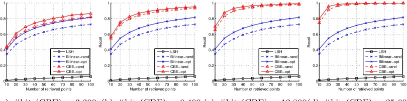
Figure 2: Recall on ImageNet-25600. The standard deviation is within 1%. First Row: Fixed time. “# bits” is the number of bits of CBE. Other methods are using fewer bits to make their computational time identical to CBE. Second Row: Fixed number of bits. CBE-opt/CBE-rand are 2-3 times faster than Bilinear-opt/Bilinear-rand, and hundreds of times faster than LSH.
7.2 Retrieval
The recalls of different methods are compared on the three data sets, shown in Figure 1 – 3. The top row in each figure shows the performance of different methods when the code generation time for all the methods is kept the same as that of CBE. For a fixed time, the proposed CBE yields much better recall than other methods. Even CBE-rand outperforms LSH and Bilinear code by a large margin. The second row compares the performance for different techniques with codes of same length. In this case, the performance of CBE-rand is almost identical to LSH even though it is hundreds of time faster. This is consistent with our analysis in Section 4. Moreover, CBE-opt/CBE-rand outperform Bilinear-opt/Bilinear-rand in addition to being 2-3 times faster.
10 20 30 40 50 60 70 80 90 100 0 0.2 0.4 0.6 0.8 1 Recall
Number of retrieved points LSH Bilinear−rand Bilinear−opt CBE−rand CBE−opt
(a) #bits(CBE) = 6,400
10 20 30 40 50 60 70 80 90 100 0 0.2 0.4 0.6 0.8 1 Recall
Number of retrieved points LSH Bilinear−rand Bilinear−opt CBE−rand CBE−opt
(b) #bits(CBE) = 12,800
10 20 30 40 50 60 70 80 90 100 0 0.2 0.4 0.6 0.8 1 Recall
Number of retrieved points LSH Bilinear−rand Bilinear−opt CBE−rand CBE−opt
(c) #bits(CBE) = 25,600
10 20 30 40 50 60 70 80 90 100 0 0.2 0.4 0.6 0.8 1 Recall
Number of retrieved points LSH Bilinear−rand Bilinear−opt CBE−rand CBE−opt
(d) #bits(CBE) = 51,200
10 20 30 40 50 60 70 80 90 100 0 0.2 0.4 0.6 0.8 1 Recall
Number of retrieved points LSH Bilinear−rand Bilinear−opt CBE−rand CBE−opt
(e) # bits (all) = 6,400
10 20 30 40 50 60 70 80 90 100 0 0.2 0.4 0.6 0.8 1 Recall
Number of retrieved points LSH Bilinear−rand Bilinear−opt CBE−rand CBE−opt
(f) # bits (all) = 12,800
10 20 30 40 50 60 70 80 90 100 0 0.2 0.4 0.6 0.8 1 Recall
Number of retrieved points LSH Bilinear−rand Bilinear−opt CBE−rand CBE−opt
(g) # bits (all) = 25,600
10 20 30 40 50 60 70 80 90 100 0 0.2 0.4 0.6 0.8 1 Recall
Number of retrieved points LSH Bilinear−rand Bilinear−opt CBE−rand CBE−opt
(h) # bits (all) = 51,200
Figure 3: Recall on ImageNet-51200. The standard deviation is within 1%. First Row: Fixed time. “# bits” is the number of bits of CBE. Other methods are using fewer bits to make their computational time identical to CBE. Second Row: Fixed number of bits. CBE-opt/CBE-rand are 2-3 times faster than Bilinear-opt/Bilinear-rand, and hundreds of times faster than LSH.
10 20 30 40 50 60 70 80 90 100 0 0.2 0.4 0.6 0.8 1 Recall
Number of retrieved points
LSH SKLSH ITQ SH AQBC BPBCr BPBC CBEr CBE
(a) # bits = 256
10 20 30 40 50 60 70 80 90 100 0 0.2 0.4 0.6 0.8 1 Recall
Number of retrieved points
LSH SKLSH ITQ SH AQBC BPBCr BPBC CBEr CBE
(b) # bits = 512
10 20 30 40 50 60 70 80 90 100
0 0.2 0.4 0.6 0.8 1 Recall
Number of retrieved points
LSH SKLSH ITQ SH AQBC Bilinear−rand Bilinear−opt CBE−rand CBE−opt
(c) # bits = 1,024
10 20 30 40 50 60 70 80 90 100
0 0.2 0.4 0.6 0.8 1 Recall
Number of retrieved points
LSH SKLSH ITQ SH AQBC Bilinear−rand Bilinear−opt CBE−rand CBE−opt
(d) # bits = 2,048
Figure 4: Performance comparison on relatively low-dimensional data (Flickr-2048) with fixed number of bits. CBE gives comparable performance to the state-of-the-art even on low-dimensional data as the number of bits is increased. However, these other methods do not scale to very high-dimensional data setting which is the main focus of this work.
10 20 30 40 50 60 70 80 90 100 Number of retrieved points 0.3
0.4 0.5 0.6 0.7 0.8 0.9 1
Recall
LSH CBE-rand CBE-opt FBE FJLT-0.05 FJLT-0.1
(a) # bits = 5,000
10 20 30 40 50 60 70 80 90 100 Number of retrieved points 0.3
0.4 0.5 0.6 0.7 0.8 0.9 1
Recall
LSH CBE-rand CBE-opt FBE FJLT-0.05 FJLT-0.1
(b) # bits = 10,000
10 20 30 40 50 60 70 80 90 100 Number of retrieved points 0.3
0.4 0.5 0.6 0.7 0.8 0.9 1
Recall
LSH CBE-rand CBE-opt FBE FJLT-0.05 FJLT-0.1
(c) # bits = 15,000
Figure 5: Recall on the Flickr-25600 data set. The methods compared are rand, CBE-opt, Fast Binary Embedding (FBE), Fast Johnson-Lindenstruss Transformation (FJLT) based methods and LSH. We follow the detailed setting of the FBE pa-per(Yi et al., 2015). In FJLT-p,p represents the percentage of nonzero elements in the sparse Gaussian matrix.
Johnson-Lindenstrss Transformation (FJLT). Similar to the circulant projection, FJLT has been used in dimensionality reduction (Ailon and Chazelle, 2006), deep neural networks (Yang et al., 2015), and kernel approximation (Le et al., 2013). Here, the binary code of
x∈Rdis generated as
h(x) = sign(PHDx), (53)
whereP∈Rk×dis a sparse matrix with the nonzeros entries generated iid from the standard
distribution. H ∈ Rd×d is the Hadamard matrix, and D ∈
Rd×d is a diagonal matrix
with random signs. Although the Hadamard transformation has computational complexity
O(dlogd) (the multiplication with H), this method is often slower than CBE due to the sparse Gaussian projection step (i.e., multiplication byP).
The second method we compare with is Fast Binary Embedding (FBE). It is a theo-retically sound method recently proposed in (Yi et al., 2015). FBE generates binary bits using a partial Walsh-Hadamard matrix and a set of partial Gaussian Toeplitz matrices. The method can achieve the optimal measurement complexityO(δ12 logN). Different from
Original LSH Bilinear-opt CBE-opt 25.59±0.33 23.49±0.24 24.02±0.35 24.55±0.30
Table 3: Multiclass classification accuracy (%) on binary coded ImageNet-25600. The bi-nary codes of same dimensionality are 32 times more space efficient than the original features (single-float).
7.3 Classification
Besides retrieval, we also test the binary codes for classification. The advantage is to save on storage, allowing even large scale data sets to fit in memory (Li et al., 2011; S´anchez and Perronnin, 2011). We follow the asymmetric setting of (S´anchez and Perronnin, 2011) by training linear SVM on binary code sign(Rx), and testing on the original Rx. Empirically, this has been shown to give better accuracy than the symmetric procedure. We use ImageNet-25600, with randomly sampled 100 images per category for training, 50 for validation and 50 for testing. The code dimension is set as 25,600. As shown in Table 3, CBE, which has much faster computation, does not show any performance degradation compared with LSH or bilinear codes in classification task.
8. Conclusion
We proposed a method of binary embedding for high-dimensional data. Central to our framework is to use a type of highly structured matrix, the circulant matrix, to perform the linear projection. The proposed method has time complexity O(dlogd) and space complexityO(d), while showing no performance degradation on real-world data compared with more expensive approaches (O(d2) orO(d1.5)). The parameters of the method can be randomly generated, where interesting theoretical analysis was carried out to show that the angle preserving quality can be as good as LSH. The parameters can also be learned based on training data with an efficient optimization algorithm.
Appendix A. Proofs of the Technical Lemmas
A.1 Proof of Lemma 6
For convenience, defineu⊥=u−Πu, and similarly define v⊥. From our earlier obser-vation about independence, we have that
E
1−sign(rTa) sign(rTb)
2 −
θ π
1−sign(rTu⊥) sign(rTv⊥)
2 −
θ π
= 0. (54)
Because the LHS is equal to the product of the expectations, and the first term is 0. Thus the quantity we wish to bound is
E
1−sign(rTa) sign(rTb)
2 −
θ π
sign(rTu) sign(rTv)−sign(rTu⊥) sign(rTv⊥) 2
Now by using the fact that E[XY] ≤ E[|X||Y|], together with the observation that the
quantity|(1−sign(rTa) sign(rTb))/2−θ/π|is at most 2, we can bound the above by
E
h
|sign(rTu) sign(rTv)−sign(rTu⊥) sign(rTv⊥)|i. (55)
This is equal to
2 Pr[sign(rTu) sign(rTv)6= sign(rTu⊥) sign(rTv⊥)], (56)
since the term in the expectation is 2 if the product of signs is different, and 0 otherwise. To bound this, we first observe that for any two unit vectorsx,ywith∠(x,y)≤, we have Pr[sign(rTx)6= sign(rTy)]≤/π. We can use this to say that
Pr[sign(rTu)6= sign(rTu⊥)] = ∠(u,u
⊥)
π . (57)
This angle can be bounded in our case by (π/2)·δ by basic geometry.10 Thus by a union bound, we have that
Pr[ sign(rTu)6= sign(rTu⊥)∨ sign(rTv)6= sign(rTv⊥)]≤δ. (58)
This completes the proof.
A.2 Proof of Lemma 7
Denoting the ith entry ofp by pi (so also forq), we have that
S :=hDp, s→t(Dq)i= d−1
X
i=0
σiσi+tpiqi+t. (59)
We note thatE[S] = 0, by linearity of expectation (ast >0,E[σiσi+t] = 0), thus the lemma
is essentially a tail bound onS. While we can appeal to standard tail bounds for quadratic forms of sub-Gaussian random variables (e.g. Hansen-Wright (Rudelson and Vershynin, 2013)), we give below a simple argument. Let us define
f(σ0, σ1, . . . , σd−1) =
d−1
X
i=0
piqi+tσiσi+t. (60)
We will view f as being obtained from a martingale as follows. Define
Qi :=f(σ0, σ1, . . . , σi,0, . . . ,0)−f(σ0, σ1, . . . , σi−1,0, . . . ,0). (61)
In this notation, we haveS =Q0+Q1+· · ·+Qd−1.
We have the martingale property that E[Qi|Q0, Q1, . . . , Qi−1] = 0 for all i, (because σi is ±1 with equal probability). Further, we have the bounded difference property, i.e.,
|Qi| ≤ |piqi+t|+|pi−tqi|. This implies that
|Qi|2 ≤2(p2iqi2+t+p2i−tq2i). (62)
Thus we can use Azuma’s inequality to conclude that for anyγ >0,
Pr[|X i
Qi−E[
X
i
Qi]|> γ]< e
− γ2
2·P
i2(p2iq2i+t+p2i−tqi2) =e
− γ2
8P2
ip2iqi2+t. (63)
We can now use the fact that P
ip2iq2i+t ≤ρ2
P
ip2i =ρ2 (sincekpk2 = 1 andkqk∞ ≤ρ).
This establishes the lemma.
A.3 Proof of Lemma 9
First, using Lemma 7 we have, for any i6=j andc >0,
Pr[|hXi, Yji|> c]< e−c
2/8ρ2
. (64)
We have a similar bound for Pr[|hXi, Xji|> c]. Thus by setting c = 4ρ
p
log(k/δ) (δ as in the statement of the lemma), we can take a union bound over all k2 choices of i6= j and conclude that w.p. at least 1−δ, we have
max
i6=j {|hXi, Xji|,|hXi, Yji|}<4ρ
p
log(k/δ). (65)
We now prove that whenever Eq. (65) holds, we obtain (γ, k) orthogonality for the desired
γ. Let us start with a basic fact in linear algebra.
Lemma 11 Let A be an d×k matrix with σk(A) ≥ τ, for some parameter τ. Then any
unit vector in the column span of A can be written as P
iαiAi, with
P
iα2i ≤1/τ2.
Proof By the definition ofσk, we have that for any αi, kPiαiAik22 ≥τ2
P
iα2i
. Thus for any unit vector P
iαiAi, we have
P
iα2i ≤1/τ2.
Now let B be the d×2k matrix whose columns are X1, Y1, X2, Y2, . . . , Xk, Yk in that
order. Consider the entries of BTB. Since Xi, Yi are unit vectors, the diagonals are all
1. The (2i−1,2i)th and (2i,2i−1)th entries are exactly cosθ, because the angle between
Xi, Yi isθ. The rest of the entries are of magnitude< η := 4ρ
p
log(k/δ).
Thus if we consider M = BTB−I (diagonal removed from BTB), we have −(cosθ+
kη)I M (cosθ+kη)I (diagonal dominance). Thus we conclude that BTB has all its eigenvalues ≥ 1−cosθ−kη. Since θ ∈ (0, π/2), we can use the standard inequality cosθ <1−θ2/2 to conclude that the eigenvalues are ≥θ2/2−kη. Now by our assumption
on ρ, we have thatkη < θ2/4. This implies that all the eigenvalues are ≥θ2/4.
Thus we have σ22k(B) ≥θ2/4. We prove now that this lets us obtain a decomposition that helps us prove (γ, k)-orthogonality. A crucial observation is the following.
Lemma 12 The projection of Xi onto span{X1, Y1, X2, Y2, . . . , Xi−1, Yi−1} has length at
most 2η
√ 2k
θ .
Proof LetS denote span{X1, Y1, . . . , Xi−1, Yi−1}. By definition, the squared of the length
of projection is equal to max{hy, Xii2 | y ∈ S andkyk2 = 1} (this is how the projection
To bound this, consider any unit vector y∈ S, and suppose we write it asP
j<iαjXj+
βjYj. Let B0 be the matrix that has columns Xj, Yj, j < i. Then it is straightforward to
see that σ2(i−1)(B0) ≥ σ2k(B) ≥ θ/2. Thus Claim 11 implies that
P
j<iαj2+βj2 ≤ 4/θ2.
This means that
hXi, yi2 =
X
j<i
αjhXj, Xii+βjhYj, Xii
2
(66)
≤ X
j<i
α2j +β2j X
j<i
hXj, Xii2+hYj, Xii2
(67)
≤ 4
θ2 ·(2i−2)η
2. (68)
(In the first step, we used Cauchy-Schwartz.) Taking square roots now gives the claim.
Now we perform the following procedure on the vectors (it is essentially Gram-Schmidt orthonormalization, with the slight twist that we deal withXi, Yi together):
1. Initialize: u1 =X1, e1 = 0, v1 =Y1, f1 = 0.
2. Fori= 2, . . . , k, we setui,vi to be the projections ofXi, Yi (respectively) orthogonal
to span{X1, Y1, . . . , Xi−1, Yi−1}. Setei=Xi−ui and fi=Yi−vi.
The important observation is that for any i, we have
span{uj,vj :j < i}= span{uj,vj,ej,fj :j < i}= span{Xj, Yj :j < i}. (69)
This is because by definition, ei,fi ∈span{Xj, Yj : j < i} for all i. Thus we have thatui
and vi satisfy the first condition in Definition 8. It just remains to analyze the lengths.
Now we can use Claim 12 to conclude that
keik22,kfik22< 8kη
2 θ2 =
128·kρ2log(k/δ)
θ2 . (70)
Once again, we use the bound on ρ to conclude that this quantity is at most 16ρ. This completes the proof of Lemma 9, withγ = 4√ρ.
A.4 Proof of Lemma 10
We start with a simple claim about the angle between ui and vi.
Lemma 13 For all i, we have ∠(ui,vi)∈(θ−πγ, θ+πγ).
Proof The angle between Xi and ui is at most sin−1(γ) < (π/2)γ. So also, the angle
between Yi and vi is at most (π/2)γ. Thus the angle between ui,vi is in the interval
(θ−πγ, θ+πγ) (by triangle inequality for the geodesic distance).
Letη >0 be a parameter we will fix later (it will be a constant timesγplog(k/δ)). For all i, we define the following events:
Ei : min{hr,uii,hr,vii}< η (71)
Fi : ¬Ei and signhr,uii 6= signhr,vii (72)
Lemma 14 For any i, we have
Pr[Ei]≤2η, (73)
Pr[Fi]∈
θ
π −πγ−2η, θ π
(74)
Proof The first inequality follows from the small ball probability of a univariate Gaussian
(since hr,uii is a Gaussian of unit variance), and the second follows from Claim 13 and (73).
We will set η to be larger than πγ, so the RHS in (74) can be replaced with (θ/π−
3η,θ/π). Furthermore, the events above for a given idepend onlyon the projection of rto
span{ui,vi}; thus they are independent for differenti. Let us abuse notation slightly and denote by Ei also the indicator random variable for the event Ei (so also Fi). Then by
standard Chernoff bounds, we have for anyτ >0,
Pr
"
X
i
Ei ≥2kη+kτ
#
< e−kτ
2
4η+τ, (75)
Pr
"
X
i
Fi6∈
kθ
π −3kη−kτ, kθ
π +kτ
#
<2e−kτ
2
θ+τ. (76)
Finally letH denote the event:
max
i {|hr,eii|,|hr,fii|} ≥η. (77)
For any i, sincekeik < γ, we have Pr[|hr,eii|> tγ]≤e−t2/2. We can use the same bound withfi, and take a union bound over all i, to conclude that Pr[H]≤2k·e−η
2/2γ2
.
Let us call a choice of r good if neither of the events in (75)-(76) above occur, and additionallyH does not occur. Clearly, the probability of anrbeing good is at least 1−δ, providedτ andηare chosen such that the RHS of the tail bounds above are all made≤δ/4.
Before setting these values, we note that for a good r,
1
k
X
i
1{signhr, Xii 6= signhr, Yii} ∈
θ
π −3η−τ, θ
π + 2η+ 2τ
. (78)
This is because whenever Fi∧ ¬H occurs, we have signhr, Xii 6= signhr, Yii, and thus the
LHS above is at least πθ −3η −τ. Also if we have ¬H, then the only way we can have signhr, Xii 6= signhr, Yii is if either Fi occurs, or if Ei occurs (in the latter case, it is not
necessary that the signs are unequal). Thus we can upper bound the LHS by πθ + 2η+ 2τ. Let us now set the values of η and τ. From the above, we need to ensure:
kτ2
4η+τ ≥log(4/δ),
kτ2
θ+τ ≥log(8/δ), and η2
2γ2 ≥log(4k/δ). (79)
Thus we setη= 2γplog(4k/δ), and
τ ≥max
(
2 log(8/δ)
k ,
r
2θlog(8/δ)
k ,
r
8ηlog(4/δ)
k
)
For the above inequality to hold, it suffices to set
τ ≥ 8 log(1√ /δ)
k . (81)
This gives the desired bound on the deviation in the angle.
References
Dimitris Achlioptas. Database-friendly random projections: Johnson-Lindenstrauss with binary coins. Journal of Computer and System Sciences, 2003.
Nir Ailon and Bernard Chazelle. Approximate nearest neighbors and the fast Johnson-Lindenstrauss transform. In ACM Symposium on Theory of Computing, 2006.
Moses S Charikar. Similarity estimation techniques from rounding algorithms. In ACM
Symposium on Theory of Computing, 2002.
Yu Cheng, Felix Xinnan Yu, Rogerio Feris, Sanjiv Kumar, Alok Choudhary, and Shih-Fu Chang. An exploration of parameter redundancy in deep networks with circulant projections. InIEEE International Conference on Computer Vision, 2015.
Anna Choromanska, Krzysztof Choromanski, Mariusz Bojarski, Tony Jebara, Sanjiv Ku-mar, and Yann LeCun. Binary embeddings with structured hashed projections. In
Inter-national Conference on Machine Learning, 2016.
Anirban Dasgupta, Ravi Kumar, and Tam´as Sarl´os. Fast locality-sensitive hashing. In
ACM SIGKDD Conference on Knowledge Discovery and Data Mining, 2011.
Jia Deng, Wei Dong, Richard Socher, Li-Jia Li, Kai Li, and Li Fei-Fei. Imagenet: A large-scale hierarchical image database. InIEEE Conference on Computer Vision and Pattern
Recognition, 2009.
Peter Frankl and Hiroshi Maehara. The johnson-lindenstrauss lemma and the sphericity of some graphs. Journal of Combinatorial Theory, Series B, 44(3):355–362, 1988.
Y. Gong, S. Lazebnik, A. Gordo, and F. Perronnin. Iterative quantization: A procrustean approach to learning binary codes for large-scale image retrieval. IEEE Transactions on
Pattern Analysis and Machine Intelligence, (99):1, 2012a.
Yunchao Gong, Sanjiv Kumar, Vishal Verma, and Svetlana Lazebnik. Angular quantization-based binary codes for fast similarity search. InAdvances in Neural Information
Process-ing Systems, 2012b.
Yunchao Gong, Sanjiv Kumar, Henry A Rowley, and Svetlana Lazebnik. Learning binary codes for high-dimensional data using bilinear projections. InIEEE Conference on
Com-puter Vision and Pattern Recognition, 2013.
Albert Gordo and Florent Perronnin. Asymmetric distances for binary embeddings. In