A Stochastic Algorithm for Feature Selection in Pattern Recognition

A Stochastic Algorithm for Feature Selection in Pattern Recognition

S´ebastien Gadat [email protected]

CMLA, ENS Cachan

61 avenue du pr´esident Wilson

CACHAN 94235 Cachan Cedex, FRANCE

Laurent Younes [email protected]

Center for Imaging Science The Johns Hopkins University 3400 N-Charles Street

Baltimore MD 21218-2686, USA

Editor: Isabelle Guyon

Abstract

We introduce a new model addressing feature selection from a large dictionary of variables that can be computed from a signal or an image. Features are extracted according to an efficiency criterion, on the basis of specified classification or recognition tasks. This is done by estimating a probability distributionPon the complete dictionary, which distributes its mass over the more efficient, or informative, components. We implement a stochastic gradient descent algorithm, using the probability as a state variable and optimizing a multi-task goodness of fit criterion for classifiers based on variable randomly chosen according toP. We then generate classifiers from the optimal distribution of weights learned on the training set. The method is first tested on several pattern recognition problems including face detection, handwritten digit recognition, spam classification and micro-array analysis. We then compare our approach with other step-wise algorithms like random forests or recursive feature elimination.

Keywords: stochastic learning algorithms, Robbins-Monro application, pattern recognition,

clas-sification algorithm, feature selection

1. Introduction

there are many applications for which detecting the pertinent explanatory variables is critical, and as important as correctly performing classification tasks. This is the case, for example, in biology, where describing the source of a pathological state is equally important to just detecting it (Guyon et al., 2002; Golub et al., 1999).

Feature selection methods are classically separated into two classes. The first approach (filter

methods) uses statistical properties of the variables to filter out poorly informative variables. This

is done before applying any classification algorithm. For instance, singular value decomposition or independent component analysis of Jutten and H´erault (1991) remain popular methods to limit the dimension of signals, but these two methods do not always yield relevant selection of variables. In Bins and Draper (2001), superpositions of several efficient filters has been proposed to remove irrelevant and redundant features, and the use of a combinatorial feature selection algorithm has provided results achieving high reduction of dimensions (more than 80 % of features are removed) preserving good accuracy of classification algorithms on real life problems of image processing. Xing et al. (2001) have proposed a mixture model and afterwards an information gain criterion and a Markov Blanket Filtering method to reach very low dimensions. They next apply classification algorithms based on Gaussian classifier and Logistic Regression to get very accurate models with few variables on the standard database studied in Golub et al. (1999). The heuristic of Markov Blanket Filtering has been likewise competitive in feature selection for video application in Liu and Render (2003).

The second approach (wrapper methods) is computationally demanding, but often is more accu-rate. A wrapper algorithm explores the space of features subsets to optimize the induction algorithm that uses the subset for classification. These methods based on penalization face a combinatorial challenge when the set of variables has no specific order and when the search must be done over its subsets since many problems related to feature extraction have been shown to be NP-hard (Blum and Rivest, 1992). Therefore, automatic feature space construction and variable selection from a large set has become an active research area. For instance, in Fleuret and Geman (2001), Amit and Geman (1999), and Breiman (2001) the authors successively build tree-structured classifiers con-sidering statistical properties like correlations or empirical probabilities in order to achieve good discriminant properties . In a recent work of Fleuret (2004), the author suggests to use mutual information to recursively select features and obtain performance as good as that obtained with a boosting algorithm (Friedman et al., 2000) with fewer variables. Weston et al. (2000) and Chapelle et al. (2002) construct another recursive selection method to optimize generalization ability with a gradient descent algorithm on the margin of Support Vector classifiers. Another effective ap-proach is the Automatic Relevance Determination (ARD) used in MacKay (1992) which introduce a learning hierarchical prior over weights in a Bayesian Network, the weights connected to irrelevant features are automatically penalized which reduces their influence near zero. At last, an interesting work of Cohen et al. (2005) use an hybrid wrapper and filter approach to reach highly accurate and selective results. They consider an empirical loss function as a Shapley value and perform an itera-tive ranking method combined with backward elimination and forward selection. This last work is not so far from the ideas we develop in this paper.

generate randomized classifiers, where the randomization is made on the variables rather than on the training set, an idea introduced by Amit and Geman (1997), and formalized by Breiman (2001). The selection algorithm and the randomized classifier will be tested on a series of examples.

The article is organized as follows. In Section 2, we describe our feature extraction model and the related optimization problem. Next, in Sections 3 and 4, we define stochastic algorithms which solve the optimization problem and discuss its convergence properties. In Section 5, we provide several applications of our method, first with synthetic data, then on image classification, spam de-tection and on microarray analysis. Section 6 is the conclusion and addresses future developments.

2. Feature Extraction Model

We start with some notations.

2.1 Primary Notation

We follow the general framework of supervised statistical pattern recognition: the input signal,

belonging to some set

I

, is modeled as a realization of a random variable, from which several

computable quantities are accessible, forming a complete set of variables (or tests, or features)

denoted

F

=_{δ1, . . .δ_|F_|}. This set is assumed to be finite, although |

F

| can be a very large

number, and our goal is to select the most useful variables. We denote δ(I) the complete set of

features extracted from an input signal I.

A classification task is then specified by a finite partition

C

=_{C1, . . .CN}of

I

; the goal is to

predict the class from the observationδ(I). For such a partition

C

and I_∈

I

, we write

C

(I)for the

class Cito which I belongs, which is assumed to be deterministic.

2.2 Classification Algorithm

We assume that a classification algorithm, denotedA, is available, for both training and testing. We

assume thatAcan be adapted to a subsetω_⊂

F

of active variables and to a specific classification

task

C

. (There may be some restriction on

C

associated toA, for example, support vector machines

are essentially designed for binary (two-class) problems.) In training mode,Auses a database to

build an optimal classifierA_ω,C :

I

_→

C

, such that

A

_ω,C(I) only depends onω(I). We shall drop

the subscript

C

when there is no ambiguity concerning the classification problem

C

. The test mode

simply consists in the application of

A

_ωon a given signal.

We will work with a randomized version of A, for which the randomization is with respect to

the set of variablesω(see Amit and Geman, 1997; Breiman, 2001, 1998). In the training phase, this

works as follows: first extract a collection_{ω(1), . . . ,ω(n)_{}of subsets of}

_F

_{, and build the classifiers}

A_ω(1), . . . ,A_ω(n). Then, perform classification in test phase using a majority rule for these n

clas-sifiers. This final algorithm will be denoted ¯A_C =A¯(ω(1)_{, . . . ,ω}(n)_,

_C

_{). It is run with fixedω}(i)_’s,

which are obtained during learning.

Note that in this paper, we are not designing the classification algorithm,A, for which we use

existing procedures; rather, we focus on the extraction mechanism creating the random subsets of

F

. This randomization process depends on the way variables are sampled from

F

, and we will

see that the design of a suitable probability on

F

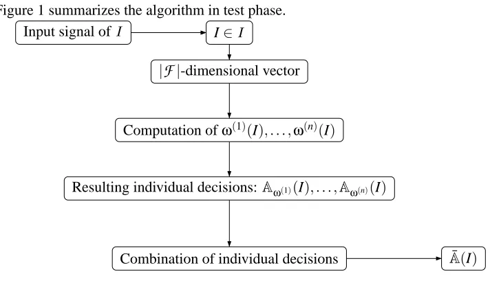
for this purpose can significantly improve the

Figure 1 summarizes the algorithm in test phase.

Input signal of

I

I_∈

I

|

F

|-dimensional vector

Computation ofω(1)(I), . . . ,ω(n)_(I)

Resulting individual decisions:A_ω(1)(I), . . . ,A_ω(n)(I)

Combination of individual decisions A¯(I)

Figure 1: Global algorithm in test phase.

2.3 Measuring the Performance of the AlgorithmA

The algorithmAprovides a different classifierA_ωfor each choice of a subsetω⊂

F

. We let q be

the classification error: q(ω,C) =P(A_ω(I)₆=

C

(I)), which will be estimated by

q?(ω,

C

) =_Pˆ₍A_ω(I)₆=

C

(I)) (1)

where ˆP is the empirical probability on the training set.

We shall consider two particular cases for a givenA.

• Multi-class algorithm: assume thatAis naturally adapted to multi-class problems (like a

q-nearest neighbor, or random forest classifier). We then let g(ω) =q?(ω,

C

)as defined above.

• Two-class algorithms: this applies to algorithms like support vector machines, which are

designed for binary classification problems. We use the idea of the one-against-all method:

denote by

Ci

the binary partition_{Ci,

I

_\Ci_}. We then denote:

g(ω) = 1

N N

∑

i=1

q?(ω,

Ci

)

which is the average classification rate of the one vs. all classifiers. This “one against all strategy” can easily be replaced by others, like methods using error correcting output codes (see Dietterich and Bakiri, 1995).

2.4 A Computational Amendment

The computation q?(ω,

C

), as defined in Equation (1), requires training a new classification

algo-rithm with variables restricted toω, and estimating the empirical error; this can be rather costly with

Because of this, we use a slightly different evaluation of the error. In the algorithm, each time

an evaluation of q?(ω,

C

) is needed, we use the following procedure (T being a fixed integer and

Ttrain

will be the training set):

1. Sample a subset

T1

of size T (with replacements) from the training set.

2. Learn the classification algorithm on the basis ofωand

T1

.

3. Sample, with the same procedure, a subset

T2

from the training set, and define ˆq_(T

1,T2)(ω,

C

)

to be the empirical error of the classifier learned via

T1

on

T2

.

Since

T1

and

T2

are independent, we will use ˆq(ω,C)defined by

ˆ

q(ω,

C

) =E_(T 1,T2)

h ˆ

q_(T

1,T2)(ω,C)

i

to quantify the efficiency of the subsetω, where the expectation is computed over all the samples

T1

,T2 of signals taken from the training set of size T . It is also clear that defining such a cost

function contributes in avoiding overfitting in the selection of variables. For the multiclass problem, we define

ˆ

g_T1,T2(ω) = 1

N N

∑

i=1

ˆ

q_(T

1,T2)(ω,

Ci

)

and we replace the previous expression of g by the one below:

g(ω) =E_T1,T2 ˆ

g_T1,T2(ω)

.

This modified function g will be used later in combination with a stochastic algorithm which will replace the expectation over the training and validation subsets by empirical averages. The

selection of smaller training and validation sets for the evaluation of ˆg_T1,T2 then represents a huge

reduction of computer time. The selection of the size of

T1

and

T2

depends on the size of the original

training set and of the chosen learning machine. It has so far been selected by hand.

In the rest of our paper, the notationE_ξ[.]will refer to the expectation usingξas the integration

variable.

2.5 Weighting the Feature Space

To select a group a variables which are most relevant for the classification task one can think first of

a hard selection method, that is, searchωsuch that

ˆ

q(ω,C) =arg min

ω∈F|ω| ˆ

q(ω,

C

).

But sampling all possible subsets (ωcovers

F

|ω|) may be untractable since_|

F

_|can be thousands

and_|ω_|ten or hundreds.

2.6 Feature Extraction Procedure

Consider a probability distributionPon the set of features

F

. For an integer k, the distributionP⊗k

corresponds to k independent trials with distributionP. We define the cost function

E

by

E

(P) =EP⊗kg(ω) =

∑

ω∈Fk

g(ω)P⊗k(ω). (2)

Our goal is to minimize this averaged error rate with respect to the selection parameter, which is

the probability distributionP. The relevant features will then be the set of variablesδ_∈

F

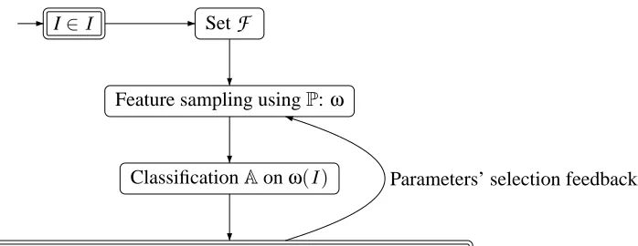
for which

P(δ) is large. The global (iterative) procedure that we propose for estimatingPis summarized in

Figure 2.

I_∈

I

Set

F

Feature sampling usingP:ω

ClassificationAonω(

I

)

Computing the mean performance g(ω)on the training set

Parameters’ selection feedback

Figure 2: Scheme of the procedure for learning the probabilityP.

Remark: We usePhere as a control parameter: we first make a random selection of features before

setting the learning algorithm. It is thus natural to optimize our way to select features from

F

and

formalize it as a probability distribution on

F

. The number of sampled features (k) is a

hyper-parameter of the method. Although we have set it by hand in our experiments, it can be estimated by cross-validation during learning.

3. Search Algorithms

We describe in this section three algorithmic options to minimize the energy

E

with respect to

the probability P. This requires computing the gradient of

E

, and dealing with the constraints

implied by the fact thatPmust be a probability distribution. These constraints are summarized in

the following notation.

We denote by

S

_F the set of all probability measures on

F

: a vectorPofR|F|belongs to

S

_F if

∑

δ∈F

P(δ) =1 (3)

and

∀δ∈

F

P(δ)_≥0. (4)

We define the projections of an element ofR|F| onto the closed convex sets

S

F and

H

F. Let

πSF(x)be the closest point of x∈R|F|in

S

F

πSF(x) =arg min

y∈SF

n

ky₋x_k22

o

and similarly

π_HF(x) =arg min

y_∈H_F

n

ky₋x_k22

o

=x₋ 1

|

F

|_δ

∑

_∈Fx(δ).

The latter expression comes from the fact that the orthogonal projection of a vector x onto a

hyper-plane is x_{− h}x,N_iN where N is the unit normal to the hyperplane. For

H

_F, N is the vector with all

coordinates equal to 1/p_|

F

_|.

Our first option will be to use projected gradient descent to minimize

E

, taking only constraint

(3) into account. This implies solving the gradient descent equation

dPt

dt =−πHF(∇

E

(Pt)) (5)

which is well-defined as long asP_{t ∈}

S

_F. We will also refer to the discretized form of (5),

P_n+1=P_n−ε_nπ_HF(∇

E

(P_n)) (6)

with positive(εn)n_∈N. Again, this equation can be implemented as long asPn∈

S

F. We will later

propose two new strategies to deal with the positivity constraint (4), the first one using the change

of variables P_7→logP, and the second being a constrained optimization algorithm, that we will

implement as a constrained stochastic diffusion on

S

F.

3.1 Computation of the Gradient

However, returning to (5), our first task is to compute the gradient of the energy. We first do it in the

standard case of the Euclidean metric on

S

_F, that is we compute∇P

E

(δ) =∂

E

/∂P(δ). Forω∈

F

k

andδ_∈

F

, denote by C(ω,δ)the number of occurrences ofδinω:

C(ω,δ) =_|{i_{∈ {}1, . . .k_{} |} ωi=δ}|.

C(ω, .)is then the_|

F

_|-dimensional vector composed by the set of values C(ω,δ),δ_∈

F

. Then, a

straightforward computation gives:

Proposition 1 IfPis any point of

S

F, then

∀δ∈

F

∇P

E

(δ) =

∑

ω∈Fk

C(ω,δ)P⊗k₍ω₎

P(δ) g(ω). (7)

Consequently, the expanded version of (6) is

P_n+1(δ) =P_n(δ)₋εn

∑

ω∈Fk

P⊗k(ω)g(ω) C(ω,δ)

P(δ) −

1

|

F

|µ

∑

_∈ω

C(ω,µ)

P(µ)

!

In the case whenP(δ) =0, then, necessarily C(ω,δ) =0 and the term C(ω,δ)/P(δ)is by convention equal to 0.

The positivity constraint is not taken in account here, but this can be dealt with, as described in the next section, by switching to an exponential parameterization. It is also be possible to design a constrained optimization algorithm, exploring the faces of the simplex when needed, but this is a rather complex procedure, which is harder to conciliate with the stochastic approximations we will describe in Section 4. This approach will in fact be computationally easier to handle with a constrained stochastic diffusion algorithm, as described in Section 3.3.

3.2 Exponential Parameterization and Riemannian Gradient

Define y(δ) =logP(δ)and

Y

=

(

y= (y(δ),δ_∈

F

) _|

∑

δ∈F

ey(δ)=1 )

which is in one-to-one correspondence with

S

F (allowing for the choice y(δ) =₋∞). Define

˜

E

(y) =

E

(P) =

∑

ω∈Fk

ey(ω1)+···+y(ωk)_g(ω_).

Then, we have:

Proposition 2 The gradient of

E

with respect to these new variables is given by:

∇y

E

˜(δ) =

∑

ω∈Fk

ey(ω1)+···+y(ωk)_C(ω_,δ_)g(ω_{). (9)}

We can interpret this gradient on the variables y as a gradient on the variablesPwith a

Rieman-nian metric

hu,v_iP=

∑

δ∈F

u(δ)v(δ)/P(δ).

The geometry of the space

S

_F with this metric D has the property that the boundary points∂

S

_F are

at infinite distance from any point into the interior of

S

F.

Denoting ˜∇for the gradient with respect to this metric, we have in fact, with y=logP:

˜

∇P

E

(δ) =∇_yE˜ =

∑

ω∈Fk

P⊗k(ω)C(ω,δ)g(ω).

To handle the unit sum constraint, we need to project this gradient on the tangent space to

Y

at

point y. Denoting this projection byπy, we have

πy(w) =w− hw|eyi/keyk2

where eyis the vector with coordinates ey(δ). This yields the evolution equation in the y variables

dyt(δ)

dt =−∇yt

E

˜(δ) +κte

where

κt=

∑

δ0_∈F

∇yt

E

˜(δ0)e

yt(δ0)

!

/

∑

δ0_∈F

e2yt(δ0)

!

does not depend onδ.

The associated evolution equation forPbecomes

dP_t(δ)

dt =−Pt(δ) ∇˜Pt

E

(δ)−κtPt(δ)

. (11)

Consider now a discrete time approximation of (11), under the form

P_n+1(δ) =Pn(δ)

Kn e

−εn(∇˜P_nE(δ)−κnPn(δ)) ₍₁₂₎

where the newly introduced constant Knensures that the probabilities sum to 1. This provides an

alternative scheme of gradient descent on

E

which has the advantage of satisfying the positivity

constraints (4) by construction.

• Start withP₀=

U

_{F 7−→}y0=logP0,

• Until convergence: ComputePn+1from Equation (12).

Remark: In terms of yn, (12) yields

yn+1(δ) =yn(δ)−εn ∇˜P_n

E

(δ)−κ_nP_n(δ)

−log Kn.

The definition of the constant Knimplies that

Kn=

∑

δ∈F

P_ne−εn(∇˜P_nE(δ)−κnPn(δ))_.

We can write a second order expansion of the above expression to deduce that

Kn=

∑

δ∈F

Pn(δ)−εnPn(δ) ∇˜P_n

E

(δ)−κ_nP_n(δ)

+Anε2_n=1+Anε2_n

since, by definition ofκn:

∑

δ∈F

P_n(δ)(∇˜P_nE(δ)−κ_nP_n(δ)) =0.

Consequently, there exists a constant B which depends on k and max(εn) such that, for all n,

|log Kn| ≤Bε2n.

3.3 Constrained Diffusion

The algorithm (8) can be combined with reprojection steps to provide a consistent procedure. We

implement this using a stochastic diffusion process constrained to the simplex

S

_F. The associated

stochastic differential equation is

dP_t=₋∇P_t

E

dt+

√_σ

where

E

is the cost function introduced in (2),σis a positive non-degenerate matrix on

H

F and dZt

is a stochastic process which accounts for the jumps which appear when a reprojection is needed.

In other words, d_|Zt|is positive if and only ifPthits the boundary∂

S

F of our simplex.

The rigorous construction of such a process is linked to the theory of Skorokhod maps, and can be found in works of Dupuis and Ishii (1991) and Dupuis and Ramanan (1999). Existence and uniqueness are true under general geometric conditions which are satisfied here.

4. Stochastic Approximations

The evaluation of∇

E

in the previous algorithms requires summing the efficiency measures g(ω)

over allωin

F

k. This is, as already discussed, an untractable sum. This however can be handled

using a stochastic approximation, as described in the next section.

4.1 Stochastic Gradient Descent

We first recall general facts on stochastic approximation algorithms.

4.1.1 APPLYING THEODE METHOD

Stochastic approximations can be seen as noisy discretizations of deterministic ODE’s (see Ben-veniste et al., 1990; Bena¨ım, 2000; Duflo, 1996). They are generally expressed under the form

Xn+1=Xn+εnF(Xn,ξn+1) +ε2nηn (13)

where Xn is the current state of the process,ξn+1 a random perturbation, andηna secondary error

term. If the distribution of ξn+1 only depends on the current value of Xn (Robbins-Monro case),

then one defines an average drift X_7→G(X)by

G(X) =E_ξ[F(X,ξ)]

and the Equation (13) can be shown to evolve similarly to the ODE ˙X=G(X), in the sense that the

trajectories coincide when(εn)n∈Ngoes to 0 (a more precise statement is given in Section 4.1.4).

4.1.2 APPROXIMATIONTERMS

To implement our gradient descent equations in this framework, we therefore need to identify two

random variables dnor ˜dnsuch that

E[dn] =πH_F[∇P_n

E

] and E

_˜

dn

=πyn

∇yn

E

˜

. (14)

This would yield the stochastic algorithm:

P_n+1=P_n−ε_ndnorPn+1=Pn e−εnd˜n

Kn .

¿From (7), we have:

∇P

E

(δ) =E_ω

C(ω,δ)g(ω)

P(δ)

Using the linearity of the projectionπ_HF, we get

π_HF(∇

E

(P)) (δ) =E_ω

π_HFC(ω, .)g(ω)

P(.)

(δ)

.

Consequently, following (14), it is natural to define the approximation term of the gradient descent (5) by:

dn=π_HF

_C(ω

n, .)qˆTn

1,T2n(ωn,

C

) P_n(.)

(15)

where the set of k featuresωnis a random variable extracted from

F

with lawPn⊗kand

T

1n,

T

2nare

independently sampled into the training set

T

.

In a similar way, we can compute the approximation term of the gradient descent based on (9) since

∇y

E

˜(δ) =Eω[g(ω)C(ω,δ)]

yielding

˜

dn=πyn

C(ωn, .)qˆTn

1,T2n(ωn,

C

))

whereπy is the projection on the tangent space

T Y

to the sub-manifold

Y

at point y, andωnis a

random variable extracted from

F

with the lawP⊗k

n .

By construction, we therefore have the proposition

Proposition 3 The mean effect of random variables dn and ˜dn is the global gradient descent, in other words:

E[dn] =π_HF (∇

E

(P_n))

and

E[dn˜] =πyn ∇

E

˜(yn)

.

4.1.3 LEARNING THEPROBABILITYMAP(Pn)n_∈N

We now make explicit the learning algorithms for Equations (5) and (10). We recall the definition of

C(ω,δ) =_|{i_{∈ {}1, . . .k_{} |} ωi=δ}|

whereδis a given feature andωa given feature subset of length k which is an hyperparameter (see

bottom of page 6). ˆq_T1,T2(ω,

C

), which is the empirical classification error on

T2

for a classifier

trained on

T1

using features inω.

•Euclidean gradient (Figure 3):

•Riemannian Gradient: For the Riemannian case, we have to give few modifications for the update

step (Figure 4).

The mechanism of the two former algorithms summarized by Figures 3,4 can be intuitively explained looking carefully at the update step. For instance, in the first case, at step n, one can see

that for all features ofδ_∈ωn, we substract fromPn(δ)amount proportional to the error performed

with ω and inversely proportional to P_n(δ) although for other features out of ωn, weights are a

little bit increased. Consequently, worst features with poor error of classification will be severely

Let

F

= (δ1, . . .δ_|F|), integers µ,T and a real numberα(stoping criterion)

n=0: defineP₀to be the uniform distribution

U

_F on

F

.

WhileP_n−bn/µc−P_n

∞>αandPn≥0:

Extractωnwith replacement from

F

k with respect toP⊗nk.

Extract

T

₁nand

T

₂nof size T with uniform independent samples over

Ttrain

.

Compute ˆq_Tn

1,T2n(ωn,

C

)and the drift vector dnwhere

dn(δ) =qˆ_Tn

1,T2n(ωn,

C

)

C(ωn,δ)

P_n(δ) −_µ

∑

_∈ω n

C(ωn,µ)

|

F

|P_n(µ)

!

.

UpdateP_n+1withP_n+1=P_n−ε_n.dn.

n_7→n+1.

Figure 3: Euclidean gradient Algorithm.

Remark We provide the Euclidean gradient algorithm, which is subject to failure (one weight might

become nonpositive) because it may converge for some applications, and in these cases, is much faster than the exponential formulation.

4.1.4 CONVERGENCE OF THEAPPROXIMATIONSCHEME

This more technical section can be skipped without harming the understanding of the rest of the paper. We here rapidly describe in which sense the stochastic approximations we have designed converge to their homologous ODE’s. This is a well-known fact, especially in the Robbins-Monro case that we consider here, and the reader may refer to works of Benveniste et al. (1990); Duflo (1996); Kushner and Yin (2003), for more details. We follow the terminology employed in the approach of Benaim (1996).

Fix a finite dimensional open set E. A differential flow(t,x)_7→φt(x)is a time-indexed family of

diffeomorphisms satisfying the semi-group conditionφt+h=φh◦φt andφ0=Id;φt(x)is typically

given as the solution of a differential equation dy_dt =G(y), at time t, with initial condition y(0) =x.

Asymptotic pseudotrajectories of a differential flow are defined as follows:

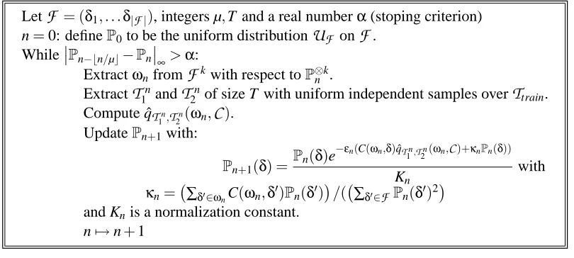
Let

F

= (δ1, . . .δ_|F_|), integers µ,T and a real numberα(stoping criterion)

n=0: defineP0to be the uniform distribution

U

F on

F

.

WhileP_n−bn/µc−P_n

_∞>α:

Extractωnfrom

F

k with respect toP⊗nk.

Extract

T

₁nand

T

₂nof size T with uniform independent samples over

Ttrain

.

Compute ˆq_Tn

1,T2n(ωn,

C

).

UpdatePn+1with:

P_n+1(δ) =Pn(δ)e

−εn(C(ωn,δ)qˆTn

1,T2n(ωn,C)+κn

P_n(δ₎₎

Kn

with

κn= ∑δ0_∈ωnC(ωn,δ0)Pn(δ0)

/( ∑_δ0_∈FPn(δ0)2

and Knis a normalization constant.

n_7→n+1

Definition 4 A map X :R+_7−→E is an asymptotic pseudotrajectory of the flowφif, for all positive numbers T

lim

t7→∞_0≤sup_h≤TkX(t+h)−φh(X(t))k=0.

In other words, the tails of the trajectory X asymptotically coincides, within any finite horizon T , with the flow trajectories.

Consider algorithms of the form

Xn+1=Xn+εnF(Xn,ξn+1) +ε2nηn+1

with Xn∈E,ξn+1a first order perturbation (such that the conditional distribution knowing all present

and past variables only depends on Xn), andηna secondary noise process. The variable Xncan be

linearly interpolated into a time-continuous process as follows: defineτn=

n

∑

k=1

εkand Xτn=Xn; then

let Xt be linear and continuous betweenτnandτn+1, for n≥0.

Consider the mean ODE

dx

dt =G(x) =Eξ[F(X,ξ)|X=x]

and its associated flowφ. Then, under mild conditions on F andηn, and under the assumption that

∑

n>0

ε1+α

n <∞for someα>0, the linearly interpolated process Xt is an asymptotic pseudotrajectory

of φ. We will consequently choose εn =ε/(n+C) where ε and C are positive constants fixed

at start of our algorithms. We can here apply this result with Xn=yn, ξn+1= (ωn,

T

1n,

T

2n) and

ηn+1=log Kn/ε2n for which all the required conditions are satisfied since for the Euclidean case,

whenωn∼P⊗nkand(

T1,T2

)∼

U

T⊗2T:

E_ωn[F(P_n,ωn)] =Eωn,T1,T2[dn(ωn,T1,T2)]

=E_ωn,T 1,T2

π_HFC(ωn, .)qˆT1,T2(ωn,

C

) P_n(.)

=E_ωn

"

π_HF C(ωn, .)ET1,T2

ˆ

q_T1,T2(ωn,

C

)

P_n(.)

!#

=E_ωn

π_HFC(ωn, .)qˆ(ωn,

C

) Pn(.)

E_ωn[F(P_n,ωn)] =πH_F(∇

E

(Pn)).

4.2 Numerical Simulation of the Diffusion Model

We use again (15) for the approximation of the gradient of

E

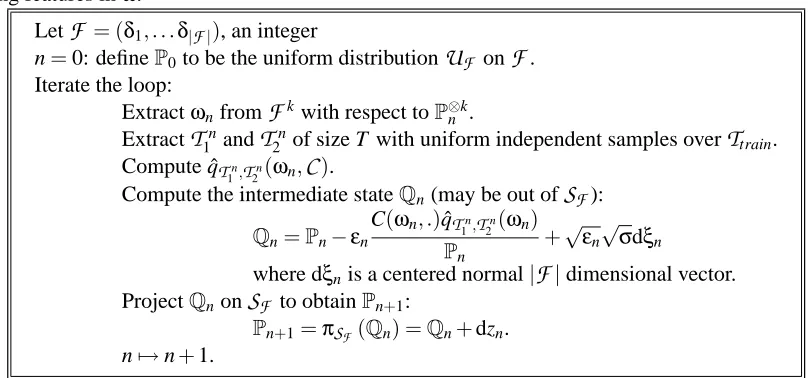
. The theoretical basis for the

conver-gence of this type of approximation can be found in Buche and Kushner (2001) and Kushner and Yin (2003), for example. A detailed convergence proof is provided in Gadat (2004).

This results in the following numerical scheme. We recall the definition of

and of ˆq_T1,T2(ω,

C

),which is the empirical classification error on

T2

for a classifier trained on

T1

using features inω.

Let

F

= (δ1, . . .δ_|F_|), an integer

n=0: defineP₀to be the uniform distribution

U

F on

F

.

Iterate the loop:

Extractωnfrom

F

k with respect toP⊗nk.

Extract

T

₁nand

T

₂nof size T with uniform independent samples over

Ttrain

.

Compute ˆq_Tn

1,T2n(ωn,

C

).

Compute the intermediate stateQ_n(may be out of

S

_F):

Q_n=P_n−ε_nC(ωn, .)qˆT

n

1,T2n(ωn)

P_n +

√_ε

n√σdξn

where dξnis a centered normal|

F

|dimensional vector.

ProjectQ_non

S

_F to obtainP_n+1:

P_n+1=π_SF(Q_n) =Q_n+dzn. n_7→n+1.

Figure 5: Constrained diffusion.

4.3 Projection on

S

_F

The natural projection on

S

_F can be computed in a finite number of steps as follows.

1. Define X0=X , if X0does not belong to the hyperplane

H

F, project first X0to

H

F:

X1=π_HF(X0).

2. – If Xk belongs to

S

_F, stop the recursion.

– Else, call Jkthe set of integers i such that X_ik_≤0 and define Xk+1by

∀i_∈Jk X_ik+1=0.

∀i_∈/Jk X_ik+1=X_ik+ 1

|

F

| − |Jk_| 1−

∑

j∈/Jk

Xk_j

!

.

One can show that the former recursion stops in at most|

F

|steps (see Gadat, 2004, chap. 4).

5. Experiments

This section provides a series of experimental results using the previous algorithms. Table 1 briefly summarizes the parameters of the several experiments performed.

5.1 Simple Examples

Data Set Dim. A Classes Training Set Test Set

Synthetic 100 N.N. 3 500 100

IRIS 4 CART 3 100 50

Faces 1926 SVM 2 7000 23000

SPAM 54 N.N. 2 3450 1151

USPS 2418 SVM 10 7291 2007

Leukemia 3859 SVM 2 72 /0

ARCENE 10000 SVM 2 100 100

GISETTE 5000 SVM 2 6000 1000

DEXTER 20000 SVM 2 300 300

DOROTHEA 100000 SVM 2 800 350

MADELON 500 N.N. 2 2000 600

Table 1: Characteristics of the data sets used in experiments.

5.1.1 SYNTHETICEXAMPLE

Data We consider_|

F

_|=100 ternary variables and 3 classes (similar results can be obtained with

more classes and variables). We let

I

=_{−1; 0; 1}f _{and the feature}δ

i(I)simply be the ith coordinate

of I_∈

I

. Let

G

be a subset of

F

. We define the probability distribution µ(;

G

)in

I

to be the one

for which all δin

F

are independent, δ(I) follows a uniform distribution on_{−1; 0; 1_} ifδ_6∈

G

andδ(I) =1 ifδ∈

G

. We model each class by a mixture of such distributions, including a small

proportion of noise. More precisely, for a class Ci, i=1,2,3, we define

µi(I) = q

3 µ(I;F

1

i ) +µ(I;

F

i2) +µ(I;

F

i3)

+ (1₋q)µ(I;/0)

with q=0.9 and

F

1

1 ={δ1;δ3;δ5;δ7},

F

12={δ1;δ5},

F

₁3={δ3;δ7},

F

1

2 ={δ2;δ4;δ6;δ8},

F

22={δ2;δ4},

F

23={δ6;δ8},

F

1

3 ={δ1;δ4;δ8;δ9},

F

32={δ1;δ8},

F

33={δ4;δ9}.

In other words, these synthetic data are generated with almost deterministic values on some vari-ables (which depends on the class the sample belongs to) and with a uniform noise elsewhere. We

expect our learning algorithm to put large weights on features in

F

_ijand ignore the other ones. The

algorithmAwe use in this case is an M nearest neighbour classification algorithm, with distance

given by

d(I1,I2) =

∑

δ∈ω

χ_{δ(I1)6=δ(I2)}.

This toy example is interesting because it is possible to compute the exact gradient of

E

for

small values of M and k=_|ω_|. Thus, we can compare the stochastic gradient algorithms with

the exact gradient algorithm and evaluate the speed of decay of

E

. Moreover, one can see in the

0.566 0.568 0.57 0.572 0.574 0.576 0.578 0.58

0 200 400 600 800 1000

Error rate

Iterates n

Exact Gradient Stochastic Exponential

0.44 0.46 0.48 0.5 0.52 0.54 0.56 0.58 0.6

0 200 400 600 800 1000

Error rate

Iterates n

Stochastic Exponential Stochastic Euclidean

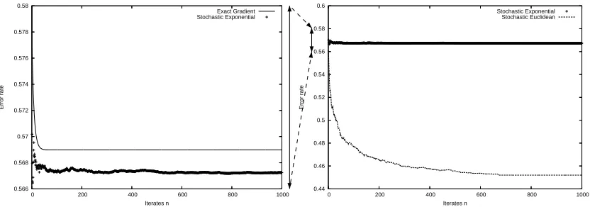
Figure 6: Note that the left and right figures are drawn on different scales. Left: Exact gradient descent (full line) vs. stochastic exponential gradient descent (dashed line) classification rates on the training set. Right: Stochastic Euclidean gradient descent (full line) vs. stochastic exponential gradient descent (dashed line) classification rates on the training set.

Results We provide in Figure 6 the evolution of the mean error

E

on our training set set against the computation time for exact and stochastic exponential gradient descent algorithms. The exact algorithm is faster but is quickly captured in a local minimum although exponential stochastic de-scent avoids more traps. Also shown in Figure 6, is the fact that the stochastic Euclidean method achieved better results faster than the exponential stochastic approach and avoided more traps than the exponential algorithm to reach lower error rates.

Note that Figure 6 (and similar plots in subsequent experiments) is drawn for the comparison of the numerical procedures that have been designed to minimize the training set errors. This does not relate to the generalization error of the final classifier, which is evaluated on test sets.

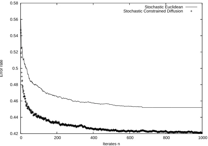
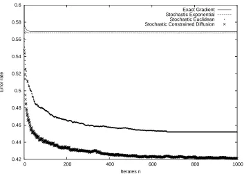
Finally, Figure 7 shows that the efficiency of the stochastic gradient descent and of the reflected diffusion are almost similar in our synthetic example. This has in fact always been so in our exper-iments: the diffusion is slightly better than the gradient when the latter converges. For this reason, we will only compare the exponential gradient and the diffusion in the experiments which follow. Finally, we summarize this instructive synthetic experiments in Figure 8. Remark that in this toy example; the exact gradient descent and the Euclidean stochastic gradient (first algorithm of Section 4.1.3) are almost equivalent.

In Figure 9, we provide the probabilities of the first 15 features in function of k=_|ω_|. (The

graylevel is proportional to the probability obtained at the limit).

Interpretation We observe that the features which are preferably selected are those which lie in

several subspaces

F

_ij, and which bring information for at least two classes. These are reusable

features, the knowledge of which being very precious information for the understanding of pattern

recognition problems. This result can be compared to selection methods based on information theory. One simple method is to select the variables which provide the most information to the class, and therefore minimize the conditional entropy (see Cover and Thomas, 1991) of the class given each variable. In this example, this conditional entropy is 1.009 for features contained in

0.42 0.44 0.46 0.48 0.5 0.52 0.54 0.56 0.58

0 200 400 600 800 1000

Error rate

Iterates n

Stochastic Euclidean Stochastic Constrained Diffusion

Figure 7: Stochastic Euclidean gradient descent (dashed line) vs. reflected diffusion (full line) clas-sification rate on the training set.

contained in two of these sets. This implies that this information-based criterion would correctly discard the non-informative variables, but fail to discriminate between the last two groups.

Remark finally that the features selected by OFW after the reusables ones are still relevant for the classification task.

5.1.2 IRIS DATABASE

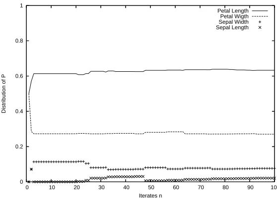
We use in this section the famous Fisher’s IRIS database where data are described by the 4 variables: “Sepal Length”, “Sepal Width”, “Petal Length” and “Petal Width”. Even though our framework is to select features in a large dictionary of variables, it will be interesting to look at the behavior of our algorithm on IRIS since results about feature selection are already known on this classical example. We use here a Classification and Regression Tree (CART) using the Gini index. We extract 2 variables at each step of the algorithm, 100 samples out of 150 are used to train our feature weighting procedure. The Figures 10 and 11 describe the behavior of our algorithms (with and without the noise term).

We remark here that for each one of our two approaches, we approximately get the entire weight on the last two variables “ Petal Length” (70%) and “Petal Width” (30%). This result is consistent with the selection performed by CART on this database since we obtain similar results as seen in Figure 12. Moreover, a selection based on the Fisher score reaches the same results for this very simple and low dimensional example.

The classification on Test Set is improved selecting two features (with OFW as Fisher Scoring)

0.42 0.44 0.46 0.48 0.5 0.52 0.54 0.56 0.58 0.6

0 200 400 600 800 1000

Error rate

Iterates n

Exact Gradient Stochastic Exponential Stochastic Euclidean Stochastic Constrained Diffusion

Figure 8: Comparison of the mean error rate computed on the test set with the 4 exact or stochastics gradient descents.

F

δ1 δ2 δ3 δ4 δ5 δ6 δ7 δ8 δ9 δ10 δ11 δ12 δ13 δ14 δ15 . . .

|ω|=2

|ω|=3

|ω|=4

Figure 9: Probability histogram for several values of_|ω_|.

of 4%. In this small low dimensional example, OFW quickly converges to the optimal weight and we obtain a ranking coherent with the selection performed by Fisher Score or CART.

5.2 Real Classification Problems

We now address real pattern recognition problems. We also compare our results with other algo-rithms: no selection method, Fisher scoring method, Recursive Feature Elimination method (RFE) of Guyon et al. (2002), L0-Norm for linear support vector machines of Weston et al. (2003) and Random Forests (RF) of Breiman (2001). We used for these algorithms Matlab implementations

provided by the Spider package for RFE and L0-SVM;1 and the random forest package of Leo

Breiman.2 _{In our experiments, we arbitrarily fixed the number of features per classifier (to 100}

for the Faces, Handwritten Digits and Leukemia data and to 15 for the email database). It would

be possible to also optimize it, through cross-validation, for example, once the optimalPhas been

0 0.2 0.4 0.6 0.8 1

0 10 20 30 40 50 60 70 80 90 100

Distribution of P

Iterates n

Petal Length Petal Wigth Sepal Width Sepal Length

Figure 10: Evolution with n of the distribution on the 4 variables using a stochastic Euclidean al-gorithm.

0 0.2 0.4 0.6 0.8 1

0 10 20 30 40 50 60 70 80 90 100

Distribution of P

Iterates n

Petal Length Petal Width Sepal Width Sepal Length

Figure 11: Evolution with n of the distribution on the 4 variables using a stochastic Euclidean dif-fusion algorithm.

computed (running this optimization online, while also estimatingPwould be too computationally

intensive). We have remarked in our experiments that the estimation ofPwas fairly robust to to

|

Petal.Length< 2.45

Petal.Width< 1.75 Petal.Length>=2.45

Petal.Width>=1.75 setosa

50/50/50

setosa 50/0/0

versicolor 0/50/50

versicolor 0/49/5

virginica 0/1/45

Figure 12: Complete classification tree of IRIS generated from recursive partitioning (CART im-plementation is using the rpart library of R).

5.2.1 FACEDETECTION

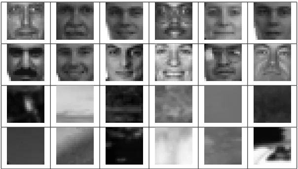
Experimental framework We use in this section the face database from MIT, which contains

19_×19 gray level images; samples extracted from the database are represented in Figure 13. The

database contains almost 7000 images to train and more than 23000 images to test.

The features in

F

are binary edge detectors, as developed in works of Amit and Geman (1999);

Fleuret and Geman (2001). This feature space has been shown to be efficient for classification in visual processing. We therefore have as many variables and dimensions as we have possible edge detectors on images. We perform among the whole set of these edge detectors a preprocessing step described in Fleuret and Geman (2001). We then obtain 1926 binary features, each one defined by its orientation, vagueness and localisation.

The classification algorithm Awhich is used here is an optimized version of Linear Support

Vector Machines developed by Joachims and Klinkenberg (2000); Joachims (2002) (with linear kernel).

Figure 13: Sample of images taken from MIT database.

1 2 3 4 5 6 7 8 9 10

20 30 40 50 60 70 80 90

Mean error rate

Number of Features k

Random Uniform Selection Stochastic Exponential

1 2 3 4 5 6 7 8 9 10

20 30 40 50 60 70 80 90

Mean error rate

Number of Features k

Random Uniform Selection Stochastic Constrained Diffusion

Figure 14: Left: Evolution with k of the average classification error of faces recognition on the

test set using a uniform law (dashed line) and P_∞(full line), learned with a stochastic

gradient method with exponential parameterization. Right: same comparison, for the constrained diffusion algorithm.

Our feature extraction method based on learning the distribution Pimproves significantly the

classification rate, particularly for weak classifiers (k=20 or 30 for example) as shown in Figure

14. We remark again that the constrained diffusion performs better than the stochastic exponential

gradient. We achieve a 1.6% error rate after learning with a reflected diffusion, or 1.7% with a

stochastic exponential gradient (2% before learning). The analysis of the most likely features (which are the most weighted variables) is also interesting, and occurs in meaningful positions, as shown in Figure 15.

Figure 16 shows a comparison of the efficiency (computed on the test set) of Fisher, RFE,

L0-SVM and our weighting procedure to select features; besides we have shown the performance ofA

without any selection and the best performance of Random Forests (as an asymptote).

We observe that our method is here less efficient with a small number of features (for 20 features

Figure 15: Representation of the main edge detectors after learning.

0 5 10 15 20 25

10 100 1000

Rate of Misclassification

Number of Features

Random Forest-1000 Trees Random Forest-100 Trees Fisher L0 OFW RFE Without Selection

Figure 16: Efficiency of several feature extractions methods for the faces database test set.

However, for a larger set of features, our weighting method is more effective than other methods

since we obtained 1.6% of misclassification for 100 features selected (2.7% for L0 selection and

The comparison with the Random Forest algorithm is more difficult to estimate: one tree

achieves 2.4% error but the length of this tree is more than 1000 and this error rate is obtained

by the 3 former algorithms using only 200 features. The final best performance on this database is

obtained using Random Forests with 1000 trees. We obtain then a misclassification rate of 0.9%.

5.2.2 SPAM CLASSIFICATION

Experimental framework This example uses a text database available at D.J. Newman and Merz (1998), which contains emails received by a research engineer from the HP labs, and divided into SPAM and non SPAM categories. The features here are the rates of appearance of some keywords (from a list of 57) in each text. As the problem is quite simple using the last 3 features of the previous list, we choose to remove these 3 variables (which depends on the number of capital letters in an email), we start consequently with a list of 54 features. We use here a 4-nearest neighbor algorithm and we extract 15 features at each step. The database is composed by 4601 messages and

we use 75% of the email database to learn our probabilityP_∞, representing our extraction method

while the 25% samples of data is left to form the test set.

0 0.05 0.1 0.15 0.2 0.25 0.3 0.35 0.4

0.1 0.12 0.14 0.16 0.18 0.2 0.22

Mean error rate

Time t

0 0.05 0.1 0.15 0.2 0.25 0.3 0.35 0.4

0.13 0.14 0.15 0.16 0.17 0.18 0.19 0.2 0.21 0.22

Time t

Mean error rate

Figure 17: Time evolution of the energy

E1

for the spam/email classification D.J. Newman and

Merz (1998) computed on the test set, using a stochastic gradient descent with an expo-nential parameterization (left) and with a constrained diffusion (right).

Results We plot the average error on the test set in Figure 17. On our test set, the method based on the exponential parameterization achieves better results than those obtained by reflected diffusion which is slower because of our Brownian noise. The weighting method is here again efficient in improving the performances of the Nearest Neighbor algorithm.

Moreover, we can analyze the words selected by our probability P_∞. In the next table, two

columns provide the features that are mainly selected. We achieve in a different way similar results to those noticed in Hastie et al. (2001) regarding the ranking importance of the words used for spam detection.

informa-Words favored for SPAM Frequency Words favored for NON SPAM Frequency

remove 8.8% cs 5.4%

business 8.7% 857 4.6%

[ 6% 415 4.4%

report 5.9% project 4.3%

receive 5.6% table 4.2%

internet 4.4% conference 4.2%

free 4.1% lab 3.9%

people 3.7% labs 3.2%

000 3.6% edu 2.8%

direct 2.3% 650 2.7%

! 1.2% 85 2.5%

$ 1% george 1.6%

Figure 18: Words mostly selected by P_∞ (exponential gradient learning procedure) for the

spam/email classification.

tions like phone numbers (“650”, “857”) or first name (“george”) are here favored to detect real email messages. The database did not provide access to the original messages, but the importance of the phone numbers or first name is certainly due to the fact that many non-spam messages are replies to previous messages outgoing from the mailbox, and would generally repeat the original sender’s signature, including its first name, address and phone number.

We compare next the performances obtained by our method with RFE, RF and L0-SVM. Figure 19 show relative efficiency of these algorithms on the spam database.

Without any selection, the linear SVM has more than 15% error rate while each one of the former feature selection algorithms achieve better results using barely 5 words. The best algorithm

is here the L0-SVM method, while the performance of our weighting method (7.47% with 20 words)

is located between RFE (11.1% with 20 words) and L0-SVM (4.47% with 20 words). In addition,

RF high performance is obtained using a small forest of 5 trees (not as deep as in the example of

faces recognition) and we obtain with this algorithm 7.24% of misclassification rate using trees of

size varying from 50 to 60 binary tests.

5.2.3 HANDWRITTENNUMBERRECOGNITION

Experimental framework A classical benchmark for pattern recognition algorithms is the classi-fication of handwritten numbers. We have tested our algorithm on the USPS database (Hastie et al., 2001; Sch¨olkopf and Smola, 2002): each image is a segment from a ZIP code isolating a single digit.

The 7291 images of the training set and 2007 of the test set are 16_×16 eight-bit grayscale maps,

with intensity between 0 and 255. We use the same feature set,

F

, as in the faces example. We

obtain a feature space

F

of 2418 edge detectors with one precise orientation, location and blurring

parameter. The classification algorithmAwe used is here again a linear support vector machine.

Results Since our reference wrapper algorithms (RFE and L0-SVM) are restricted to 2 class

prob-lems, we present only results obtained on this database with the algorithmAwhich is a SVM based

Figure 19: Efficiency of several feature extractions methods on the test set for the SPAM database.

Class

C0

C1

C2

C3

C4

C5

C6

C7

C8

C9

Image I

Figure 20: Sample of images taken from the USPS database.

The improvement of the detection rate is also similar to the previous example, as shown in Figure

21. We first plot the mean classification error rate before and after learning the probability mapP.

These rates are obtained by averaging g(ω)over samples of features uniformly distributed on

F

in

the first case, and distributed according toPin the second case. These numbers are computed on

training data and therefore serve for evaluation of the efficiency of the algorithm in improving the

energy function from

E1

(

U

F)to

E1

(P_∞). Figure 21 provides the variation of the mean error rate in

function of the number of features k used in eachω. The ratio between the two errors (before and

after learning) rates, is around 90% independently on the value of k.

Figure 22 provides the result of the classification algorithm (using the voting procedure) on the test set. The majority vote is based on 10 binary SVM-classifiers on each binary classification

problem Civs. I\Ci. The features are extracted first with the uniform distribution

U

F on

F

, then

using the finalP_∞.

The learning procedure significantly improves the performance of the classification algorithms.

3 4 5 6 7

40 50 60 70 80 90 100

Mean error rate

Number of Features k

Random Uniform Selection Stochastic Exponential 3 4 5 6 7

40 50 60 70 80 90 100

Mean error rate

Number of Features k

Random Uniform Selection Stochastic Constrained Diffusion

Figure 21: Mean error rate over the training set USPS for k varying from 40 to 100, before (dashed line) and after (full line) a stochastic gradient learning based on exponential parameter-ization (left) and constrained diffusion (right).

3 4 5 6 7 8 9

40 50 60 70 80 90 100

Mean error rate

Number of Features k

Random Uniform Selection Stochastic Exponential 3 4 5 6 7 8 9

40 50 60 70 80 90 100

Mean error rate

Number of Features k

Random Uniform Selection Stochastic Constrained Diffusion

Figure 22: Evolution with k of the mean error of classification on the test set, extraction based

on random uniform selection (dashed line) andP_∞selection (full line) for USPS data,

learning computed with stochastic gradient using exponential parameterization (left) and constrained diffusion (right).

class

Ci

, with 100 binary features per elementary classifier. The performance is not as good as

the one obtained by the tangent distance method of Simard and LeCun (1998) (2.7% error rate of

classification), but we here use very simple (edge) features. And the result is better, for example,

than linear or polynomial Support Vector Machines (8.9% and 4% error rate) computed without any

selection and than sigmoid kernels (4.1%) (see Sch ¨olkopf et al., 1995) with a reduced complexity

(measured, for example by the needed amount of memory).

Since the features we consider can be computed at every location in the image, it is interesting to visualize where the selection has occurred. This is plotted in Figure 23, for the four types of edges we consider (horizontal, vertical and two diagonal), with grey levels proportional to the value

Horizontal edges Vertical edges Diagonal edges “+π/4” Diagonal edges “₋π/4”

Figure 23: Representation of the selected features after a stochastic exponential gradient learning for USPS digits. Greyscales are proportional to weights of features

5.2.4 GENESELECTION FORLEUKEMIAAML-ALL RECOGNITION

Experimental framework We carry on our experiments with feature selection and classification for microarray data. We have used the Leukemia Database AML-ALL of Golub et al. (1999). We have a very small number of samples (72 signals) described by a very large number of genes. We run a preselection method to obtain the database used by Deb and Reddy (2003) that contains 3859

genes.3 Our algorithmAis here a linear support vector machines. As we face a numerical problem

with few samples on each class (AML and ALL), we decide to benchmark each of the algorithms we have tested using a 10-fold cross validation method.

0 0.02 0.04 0.06 0.08 0.1 0.12 0.14

0 100 200 300 400 500

Mean error rate

Time t

"leukemia"

Figure 24: Evolution of the mean energy

E

computed by the constrained diffusion method on the

training set with time for k=100.

Results Figure 24 shows the efficiency of our method of weighting features in reducing the mean

error

E

on the training set. We remark that with random uniform selection of 100 features, linear

support vector machines obtain a poor rate larger than 15% while learningP_∞, we achieve a mean

error rate less than 1%.

We now compare our result to RFE, RF and L0-SVM using the 10-fold cross validation method. Figure 25 illustrates this comparison between these former algorithms. In this example, we obtain

Figure 25: Efficiency of several feature extractions methods for the Leukemia database. Perfor-mances are computed using 10 CV.

better results without any selection, but in fact the classification of one linear SVM does not permit to rank features by importance effect on the classification task. We note here again that our weight-ing method is less effective for short size subsets (5 genes) while our method is competitive with larger subsets (20-25 genes). Here again, we note that L0-SVM outperforms RFE (like in the SPAM study Section 5.2.2). Finally, the Random Forest algorithm obtains results which are very irregular in connection with the number of trees as one can see in Figure 26.

5.2.5 FEATURESELECTIONCHALLENGE

We conclude our experiments with results on the Feature Selection Challenge described in Guyon

et al. (2004).4 Data sets cover a large field of the feature selection problem since examples are

Figure 26: Error bars of Random Forests in connection with the number of trees used computed by cross-validation.

taken in several areas (Microarray data, Digit classification, Synthetic examples, Text recognition and Drug discovery). Results are provided using the Balanced Error Rate (BER) obtained on the validation set rather than the classical error rate.

We first performed a direct Optimal Feature Weighting algorithm on theses data sets without

any feature preselection using a linear SVM for our base classifierA. For four of the five data sets

(DEXTER, DOROTHEA, GISETTE and MADELON) the numerical performances of the algorithm are significantly improved if a variable preselection is performed before running it. This preselection was based on the Fisher Score:

Fi=

(x1_{i −}xi)2+ (x2i −xi)2

1

n1−1 n1

∑

k=1

(x1_k,i−x1_i)2₊ 1 n2−1

n2

∑

k=1

(x2_k,i−x2_i)2 .

Here n1and n2are the numbers of samples of the training set of classes 1 and 2, x1i,x2i and xiassign

the mean of feature i on class 1, 2 and over the whole training set. We preselect the features with Fisher Score higher than 0.01.

We then perform our Optimal Feature Weighting algorithm with the new set of features obtained

by the Fisher preselection using forAa support vector machine with linear kernel. Figure 27 show

the decreasing evolution of the mean BER on the training set for each data sets of the feature selection challenge. One instantaneously can see that OFW is much more efficient on GISETTE or ARCENE than on other data sets since the evolution of mean BER is faster and have a larger amplitude.

For computational efficiency, our weight distribution Pis learned using a linear SVM for the

basic algorithm,A. Once this is done, an optimal nonlinear SVM is used for the final classification

0.1 0.12 0.14 0.16 0.18 0.2

0 10 20 30 40 50 60 70 80 90 100

Mean BER iterations n*1000 ’ber_arcene.train’ 0.05 0.06 0.07 0.08 0.09 0.1 0.11 0.12 0.13 0.14 0.15

0 10 20 30 40 50 60 70 80

Mean BER iterations n*1000 ’ber_dexter.train’ 0.27 0.275 0.28 0.285 0.29 0.295 0.3 0.305 0.31

0 50 100 150 200 250

Mean BER iterations n*1000 ’ber_dorothea.train’ 0.03 0.04 0.05 0.06 0.07 0.08 0.09 0.1

0 50 100 150 200 250 300

Mean BER iterations n*1000 ’ber_gisette.train’ 0.34 0.36 0.38 0.4 0.42 0.44

0 10 20 30 40 50 60 70 80 90 100

Mean BER

iterations n*1000

’ber_madelon.train’

Figure 27: Evolution with iterations n of the Balanced Error Rate on the training set.

cross validation procedure on the training set. Table 2 summarizes results obtained by our OFW

algorithm and, Linear SVM,5and others algorithms of feature selection (Transductive SVM of Wu

and Li (2006), combined filter methods with svm as F+SVM of Chen and Lin (2006) and FS+SVM of Lal et al. (2006), G-flip of Gilad-Bachrach et al. (2004), Information-Based Feature Selection of Lee et al. (2006), and analysis of redundancy and relevance (FCBF) of Yu and Liu (2004)). We select these methods since they are meta algorithms (as OFW method) whose aim is to optimize the feature subset entry of standard algorithms. These results are those obtained on the Validation Set since most of the papers previously cited do not report results on the Test Set. One can show that most of these methods outperform the performance of SVM without any selection.