In Search of Non-Gaussian Components of a High-Dimensional Distribution

(1)

In Search of Non-Gaussian Components of a

High-Dimensional Distribution

Gilles Blanchard [email protected]

Fraunhofer FIRST.IDA Kekul´estrasse 7 12489 Berlin, Germany and

CNRS, Universit´e Paris-Sud Orsay, France

Motoaki Kawanabe [email protected]

Fraunhofer FIRST.IDA Kekul´estrasse 7 12489 Berlin, Germany

Masashi Sugiyama [email protected]

Department of Computer Science Tokyo Institute of Technology

2-12-1, O-okayama, Meguro-ku, Tokyo, 152-8552, Japan

Vladimir Spokoiny [email protected]

Weierstrass Institute and Humboldt University Mohrenstrasse 39

10117 Berlin, Germany

Klaus-Robert M ¨uller [email protected]

Department of Computer Science University of Potsdam

August-Bebel-Strasse 89, Haus 4 14482 Potsdam, Germany

(2)

Abstract

Finding non-Gaussian components of high-dimensional data is an important preprocessing step for efficient information processing. This article proposes a new linear method to identify the “non-Gaussian subspace” within a very general semi-parametric framework. Our proposed method, called NGCA (non-Gaussian component analysis), is based on a linear operator which, to any arbitrary nonlinear (smooth) function, associates a vector belonging to the low dimensional non-Gaussian target subspace, up to an estimation error. By applying this operator to a family of dif-ferent nonlinear functions, one obtains a family of difdif-ferent vectors lying in a vicinity of the target space. As a final step, the target space itself is estimated by applying PCA to this family of vectors. We show that this procedure is consistent in the sense that the estimaton error tends to zero at a parametric rate, uniformly over the family, Numerical examples demonstrate the usefulness of our method.

1. Introduction

Suppose _{Xi}ni=1 are i.i.d. samples in a high dimensional space Rd drawn from an unknown

dis-tribution with density p(x). A general multivariate distribution is typically too complex to analyze directly from the data, thus dimensionality reduction is useful to decrease the complexity of the model (see Cox and Cox, 1994; Sch¨olkopf et al., 1998; Roweis and Saul, 2000; Tenenbaum et al., 2000; Belkin and Niyogi, 2003). Here, our point of departure is the following assumption: the high dimensional data includes low dimensional non-Gaussian components, and the other components are Gaussian. This assumption follows the rationale that in most real-world applications, the ‘sig-nal’ or ‘information’ contained in the high-dimensional data is essentially non-Gaussian, while the ‘rest’ can be interpreted as high dimensional Gaussian noise.

1.1 Setting and General Principle

We want to emphasize from the beginning that we do not assume the Gaussian components to be of

smaller order of magnitude than the signal components; all components are instead typically of the same amplitude. This setting therefore excludes the use of dimensionality reduction methods based

on the assumption that the data lies, say, on a lower dimensional manifold, up to some small noise. In fact, this type of methods addresses a different kind of problem altogether.

Under our modeling assumption, therefore, the task is to recover the relevant non-Gaussian components. Once such components are identified and extracted, various tasks can be applied in the data analysis process, say, data visualization, clustering, denoising or classification.

If the number of Gaussian components is at most one and all the non-Gaussian components are mutually independent, independent component analysis (ICA) techniques (see, e.g., Comon, 1994; Hyv¨arinen et al., 2001) are relevant to identify the non-Gaussian subspace. Unfortunately, however, this is often a too strict assumption on the data.

The framework we consider is on the other hand very close to that of projection pursuit (denoted PP in short in the sequel) algorithms (Friedman and Tukey, 1974; Huber, 1985; Hyv¨arinen et al., 2001). The goal of projection pursuit methods is to extract non-Gaussian components in a gen-eral setting, i.e., the number of Gaussian components can be more than one and the non-Gaussian components can be dependent.

(3)

possible directions of projection; the procedure can be repeated iteratively (over directions orthog-onal to the first ones already found) to find a higher dimensiorthog-onal projection of the data as needed.

However, it is known that some projection indices are suitable for finding super-Gaussian com-ponents (heavy-tailed distribution) while others are suited for identifying sub-Gaussian comcom-ponents (light-tailed distribution) (Hyv¨arinen et al., 2001). Therefore, traditional PP algorithms may not work effectively if the data contains, say, both super- and sub-Gaussian components.

To summarize: existing methods for the setting we consider typically proceed by defining an appropriate interestingness index, and then compute a projection that maximizes this index (projec-tion pursuit methods, and some ICA methods). The philosophy that we would like to promote in this paper is in a sense different: in fact, we do not specify what we are interested in, but we rather define what is not interesting (see also Jones and Sibson , 1987). Clearly, a multi-dimensional Gaus-sian subspace is a reasonable candidate for an undesired component (our idea could be generalized by defining, say, a Laplacian subspace to be uninformative). Having defined this uninteresting sub-space, its (orthogonal) complement is by contrast interesting: this therefore precisely defines our target space.

1.2 Presentation of the Method

Technically, our new approach to identifying the non-Gaussian subspace uses a very general semi-parametric framework. The proposed method, called non-Gaussian component analysis (NGCA), is essentially based on a central property stating that there exists a linear mapping h_7→β(h)_∈Rd

which, to any arbitrary (smooth) nonlinear function h :Rd →R, associates a vector β lying in

the non-Gaussian target subspace. In practice, the vector β(h) has to be estimated from the data, giving rise to an estimation error. However, our main consistency result shows that this estimation error vanishes at a rate plog(n)/n with the sample size n . Using a whole family of different

nonlinear functions h then yields a family of different vectorsbβ(h) which all approximately lie in, and span, the non-Gaussian subspace. We finally perform PCA on this family of vectors to extract the principal directions and estimate the target space.

In practice, we consider functions of the particular form hω,a(x) = fa(hω,xi), where f is a

function class parameterized, say, by a parameter a , and _kω_k=1 . Even for a fixed a , it is infeasi-ble to compute values of β(h_ω,a) for all possible values of ω (say, on a discretized net of the unit

sphere), because of the cardinality involved. In order to choose a relevant value forω (still for fixed

a ), we then opt to use as a heuristic a well-known PP algorithm, FastICA (Hyv¨arinen, 1999). This

was suggested by the surprising observation that the mapping ω_→β(h_ω,a) is then equivalent to a single iteration of FastICA (although this algorithm was built using different theoretical

considera-tions); hence, in this special case, FastICA is exactly the same as iterating our mapping. In short, we use a PP method as a proxy to select the most relevant directionω for a fixed a . This results in a particular choice ofωa, to which we apply the mapping once more, thus yieldingβa=β(hωa,a).

Fi-nally, we aggregate the different vectorsβa obtained when varying a by applying PCA as indicated

previously, in order to recover the target space.

Thus, apart from the conceptual point, defining uninterestingness as the point of departure in-stead of interestingness, another way to look at our method is to say that it allows the combination of information coming from different indices: here the above function fa (for fixed a ) plays a role

(4)

point here is that, while traditional projection pursuit does not provide a well-founded justification for combining directions from using different indices, our framework allows to do precisely this – thus implicitly selecting, in a given family of indices, the ones which are the most informative for the data at hand.

In the following section we will outline the theoretical cornerstone of the method, a novel semi-parametric theory for linear dimension reduction. Section 3 discusses the algorithmic procedure and is conluded with theoretical results establishing statistical consistency of the method. In Section 4, we study on simulated and real data examples the behavior of the algorithm. A brief conclusion is given in Section 5.

2. Theoretical Framework

In this section, we give a theoretical basis for the non-Gaussian component search within a

semi-parametric framework. We present a population analysis, where expectations can in principle be

calculated exactly, in order to emphasize the main idea and show how the algorithm is built. A more rigorous statistical study of the estimation error will be exposed later in section 3.5.

2.1 Motivation

Before introducing the semi-parametric density model which will be used as a foundation for devel-oping our method, we motivate it by starting from elementary considerations. Suppose we are given a set of observations Xi ∈Rd, (i=1, . . . ,n) obtained as a sum of a signal S and an independent

Gaussian noise component N :

X=S+N, (1)

where N_∼

N

(0,Γ). Note that no particular structural assumption is made about the noise covari-ance matrix Γ.

Assume the signal S is contained in a lower-dimensional linear subspace E of dimension m< d . Loosely speaking, we would like to project X linearly so as to eliminate as much of the noise as

possible while preserving the signal information. An important issue for the analysis of the model (1) is a suitable representation of the density of X which reflects the low dimensional structure of the non-Gaussian signal. The next lemma presents a generic representation of the density p for the model (1).

Lemma 1 The density p(x) for the model (1) with the m -dimensional signal S and an independent Gaussian noise N can be represented as

p(x) =g(T x)φ_Γ(x)

where T is a linear operator fromRd toRm, g(_·) is some function onRm andφΓ(x)is the density of the Gaussian component.

(5)

complementary subspace to E . In the general situation with “colored” Gaussian noise, the signal

space E does not coincide with the orthogonal complementary of the kernel

I

=K₍_T₎⊥ _{of the}

operator T . However, the density representation of Lemma 1 shows that the the subspace K₍_T₎

is non-informative and contains only noise. The original data can then be projected orthogonally

onto

I

, which we call the non-Gaussian subspace, without loss of information. This way, we are

preserving the totality of the signal information. This definition implements the general point of view outlined in the introduction, namely: we define what is considered uninteresting; the target space is then defined indirectly as the orthogonal of the uninteresting component.

2.2 Relation to ICA

An equivalent view of the same model is to decompose the noise N appearing in Eq.(1) into a

component N1 belonging to the signal space E and an independent component N2; it can then be

shown that N2 belongs to the subspace K(T) defined above. In this view, the space

I

is orthogonal

to the independent noise component, and projecting the data onto

I

amounts to cancelling this

independent noise component by an orthogonal projection.

In the present paper, we assume that we wish to project the data orthogonally, i.e., that the Euclidean geometry of the input space is meaningful for the data at hand, and that we want to respect it while projecting. An alternative point of view would be to disregard the input space geometry altogether, and to first map the data linearly to a reference space where it has covariance identity (“whitening” transform), which would be closer to a traditional ICA analysis. This would have on the one hand the advantage of resulting in an affine invariant procedure, but, on the other hand, the disadvantage of losing the information of the original space geometry. It is relatively straightforward to adapt the procedure to fit into this framework. For simplicity, we will stick to our original goal of orthogonal projection in the original space.

2.3 Main Model

Based on the above motivation, we assume to be dealing with an unknown probability density function p(x) on Rd which can put under the form

p(x) =g(T x)φ_Γ(x), (2)

where T is an unknown linear mapping from Rd to Rm with m_≤d , g is an unknown function on

Rm, and φ_Γ is a centered1Gaussian density with covariance matrixΓ.

Note that the semi-parametric model (2) includes as particular cases both the pure parametric

( m=0 ) and purely non-parametric ( m=d ) models. For practical purposes, however, we are

effectively interested in an intermediate case where d is large and m is relatively small. In what follows, we denote by

I

the m -dimensional linear subspace inRd generated by the adjoint operator

T∗:

I

=K₍_T₎⊥₌ℑ₍_T∗₎_,

where ℑ(_·) denotes the range of an operator. We call

I

the non-Gaussian subspace.

The proposed goal is therefore to estimate

I

by some subspaceb

I

computed from an i.i.d. sam-ple _{Xi}ni=1 following the distribution with density p(x). In this paper, we assume the effective 1. It is possible to handle a more general situation where the Gaussian part has an unknown mean parameter θ in

(6)

dimension m to be known or fixed a priori by the user. Note that we do not estimate Γ nor g when estimating

I

. We measure the closeness of the two subspacesb

I

and

I

by the following error function:

E

(b

I

,

I

) = (2m)−1ΠI−ΠbI

2

Frob=m− 1

∑

m

i=1

k(Id−ΠbI)vik

2_, ₍₃₎

where ΠI denotes the orthogonal projection on

I

, k·k_Frob is the Frobenius norm, {vi}m_i₌₁ is an orthonormal basis of

I

and Id is the identity matrix.

2.4 Key Result

The main idea underlying our approach is summed up in the following Proposition (the proof is given in Appendix A.2). Whenever variable X has covariance2 matrix identity, this result allows, from an arbitrary smooth real function h on Rd, to find a vectorβ(h)_∈

I

.

Proposition 2 Let X be a random variable whose density function p(x) satisfies Eq.(2) and sup-pose that h(x) is a smooth real function on Rd. Assume furthermore that Σ=EX X>=Id. Then, under mild regularity conditions on h , the following vector β(h) belongs to the target space

I

:

β(h) =E[X h(X)₋∇h(X)]. (4)

In the general case where the covariance matrix Σ is different from identity, provided it is non-degenerated, we can apply a whitening operation (also known as Mahalanobis transform). Namely, let us put Y =Σ−12X the “whitened” data; the covariance matrix of Y is then identity. Note that if

the density function of X is of the form

p(x) =g(T x)φ_Γ(x),

then by change of variable the density function of Z=AX is given by

q(z) =cAg(TA−1z)φ_A_Γ_A>(z), where cA is a normalization constant depending on A .

This identity applied to A=Σ−12 and the previous proposition allow to conclude that

βY(h) =E[∇h(y)−yh(y)]∈

J

=ℑ(Σ

1 2_T∗)

and therefore that

γ(h) =Σ−12β_Y(_h)∈

I

=ℑ(_T∗),

where

I

is the non-Gaussian index space for the initial variable X , and

J

=Σ12

I

the transformed

non-Gaussian space for the whitened variable Y .

(7)

I

h

1

2 3

4 5

β

1

β4 2

^

^ ^

3

β ^

5

h(x)

x

Figure 1: The NGCA main idea: from a varied family of real functions, compute a family of vectors belonging to the target space up to small estimation error.

3. Procedure

We now use the key proposition established in the previous section to design a practical algorithm in order to identify the non-Gaussian subspace. The first step is to apply the whitening transform to the data (where the true covariance matrix Σis estimated by the empirical covariance bΣ). We then estimate the “whitened” non-Gaussian space

J

by some b

J

(this will be described next); this space is then finally pulled back in the original space by application of bΣ−12. To simplify the exposition,

in this section we will forget about the whitening/dewhitening steps and always implicitly assume that we are dealing directly with the whitened data: every time we refer to the non-Gaussian space it is therefore to be understood that we refer to

J

=Σ12

I

, corresponding to the whitened data Y .

3.1 Principle of the Method

In the previous section, we have proved that for an arbitrary function h satisfying mild smoothness conditions, it is possible to construct a vector β(h) which lies in the non-Gaussian subspace. How-ever, since the unknown density p(x) is used (via the expectation operator) to define β by Eq.(2), one cannot directly use this formula in practice: it is then natural to approximate it by replacing the true expectation by the empirical expectation. This gives rise to the estimated vector

b

β(h) =1

n n

∑

i=1

Yih(Yi)₋∇h(Yi), (5)

which we expect to be close to the non-Gaussian subspace up to some estimation error. At this point, the natural next step is to consider a whole family of functions _{hi_}n_i₌₁, giving rise to an associated vector family of _{βbi}Li=1, all lying close to the target subspace, where bβi:=bβ(hi). The

final step is to recover the non-Gaussian subspace from this set. For this purpose, we suggest to use the principal directions of this family, i.e. to apply PCA (although other algorithmic options are certainly avalaible for this task). This general idea is illustrated on Figure 1.

3.2 Normalization of the Vectors

When extracting information on the target subspace from the set of vectors_{βbi}Li=1, attention should

be paid to how the functions {hi}L

i=1 are normalized. As can be seen from its definition, the

(8)

associ-Figure 2: For the same estimation error represented as a confidence ball of radius ε, estimated vectors with higher norm give a more precise information about the true target space.

ated bβ(h) could have an arbitrarily large norm: this is likely to influence heavily the procedure of principal direction extraction applied to the whole family.

To prevent this problem, the functions {hi}L

i=1 should be normalized in some way or other.

Several possibilities can come to mind, like using the supremum or L2 norm of h or of ∇h . We

argue here that a sensible way to normalize functions is such that the average squared deviation (estimation error) of bβ(h) to its mean is of the same order for all functions h considered. This has a first direct intuitive interpretation in terms of making the length of each estimated vector proportional to its associated signal-to-noise ratio. We argue in more detail that the norm of bβ(h)

after normalization is directly linked to the amount of information brought by this vector about the target subspace.

Namely, if we measure the information that is brought by a certain vector bβ(h) about the target space

J

through the angleθ(bβ(h))between the vector and the space, we have

kbβ(h)₋β(h)_{k ≥}dist(bβ(h),

J

) =sin(θ(bβ(h)))_kbβ(h)_k. (6)

Suppose we have ensured by renormalization that σ(h)2₌_Eh_kb_β₍_h₎₋_β₍_h₎_k2i _{is constant and}

in-dependent of h , and assume that this results in _kbβ(h)₋β(h)_k2 _{being bounded by some constant}

with high probability. It entails that sin(θ(bβ(h)))_kbβ(h)_kis bounded independently of h . We expect, in this situation, that the bigger_kbβ_k, the smaller is sin(θ), and therefore the more reliable the infor-mation about

J

. This intuition is illustrated in Figure 2, where the estimation error is represented by a confidence ball of equal size for all vectors.3

Therefore, at least at an intuitive level, it appears appropriate to use σ(h) as a renormalization. Note that this is just the square root of the trace of the covariance matrix of bβ(h), and therefore easy to estimate in practice from its empirical counterpart. In section 3.5, we give actual theoretical confidence bounds for _kβ₋bβ_k which justify this intuition in a more rigorous manner.

Finally, to confirm this idea on actual data, we plot in the top row Figure 3 the distribution of

b

β on an illustrative data set using the normalization scheme just described. In order to investigate

(9)

the relation between the norm of the (normalized) bβ and the amount of information on the non-Gaussian subspace brought by bβ, we plot in the right part of Figure 3 the relation between _kbβ_k and kΠJbβk/kbβk=cos(θ(bβ)). As expected, the vectors bβ with highest norm are indeed much closer

to the non-Gaussian subspace in general. Furthermore, vectors bβ with norm close to zero appear

to bear almost no information about the non-Gaussian space, which is consistent with the setting depicted in Figure 2: whenever an estimated vector bβ has norm smaller than the estimation errorε, its confidence ball contains the origin, which means that it brings no useable information about the direction of the non-Gaussian subspace.

These findings motivate two important points for the algorithm:

1. It should be beneficial to actively search for functions h which yield an estimated bβ(h) with higher norm, since these are more informative about the target space

J

;

2. The vectors bβ with norm below a certain threshold ε can be discarded as they are non-informative. So far, the theoretical bounds presented below in section 3.5 are not precise enough to give a canonical value for this threshold: we therefore recommend that it be de-termined by a preliminary calibration procedure. For this, we consider independent Gaussian data: in this case, β=0 for any h and thus _kbβ_k represents pure estimation noise. A reason-able choice for the threshold is therefore the 95th percentile (say) of this distribution, which we expect to reject a large majority of the noninformative vectors.

3.3 Using FastICA as Preprocessing to Find Promising Functions

When considering a parametrized family of functions _{h_ω_}, it is a desirable goal to search the parameter space to find indices ω such thatbβ(hω) has a high norm, as proposed in the last section. From now on we will restrict our attention to functions of the form

hω(x) = f(_hω,x_i), (7)

whereω∈Rd_, _kω_k₌_{1 , and f is a smooth real function of a real variable. Clearly, it is not feasible}

to sample the entire parameter space forω as soon as it has more than a few dimensions, and it is not obvious a priori to find parameters ωsuch that bβ(hω) has a high norm. Remember however that we do not need to find an exact maximum of this norm over the parameter space. We merely want to find parameters such that the associated norm is preferably high, because they bring more information; this may also involve heuristics. Naturally, good heuristics should be able to find parameters giving rise to vectors with higher norm, bringing more information on the subspace and ultimately better practical results; nevertheless, the underlying theoretical motivation stays unchanged regardless of the way the functions are picked.

A particularly relevant heuristic for choosing ω comes naturally with a closer look at Eq.(5) when we plug in functions of the specific form given by Eq.(7):

b

β(h_ω) =1

n n

∑

i=1

Yif(hω,Yii)−f0(hω,Yii)ω

. (8)

(10)

iter-−2.5 −2 −1.5 −1 −0.5 0 0.5 1 1.5 2 −1.5

−1 −0.5 0 0.5 1 1.5

0 0.5 1 1.5 2 2.5 3 3.5 4 0

0.1 0.2 0.3 0.4 0.5 0.6 0.7 0.8 0.9 1

||β^||

cos(

θ

)

−10 −5 0 5 10

−10 −8 −6 −4 −2 0 2 4 6 8 10

0 5 10 15 20 25 0

0.1 0.2 0.3 0.4 0.5 0.6 0.7 0.8 0.9 1

||β^||

cos(

θ

)

−20 −15 −10 −5 0 5 10 15 20

−15 −10 −5 0 5 10 15

0 5 10 15 20 25 30 0

0.1 0.2 0.3 0.4 0.5 0.6 0.7 0.8 0.9 1

||β^||

cos(

θ

)

(11)

ating the following update rule to form a sequenceω1, . . . ,ωT:

ωt+1∝

1

n n

∑

i=1

Yif(hωt,Yii)−f0(hωt,Yii)ωt

(9)

where the sign ∝ indicates that vectorωt+1 is renormalized to be of unit norm.

Note that the FastICA procedure is derived from quite a different theoretical setting of what we considered here (see, e.g., Hyv¨arinen et al., 2001); its goal is in principle to optimize a non-Gaussianity measure E[F(_hω,x_i)](where F is such that F0 formally coincides with our f above) and the solution is reached by an approximate Newton method giving rise to the update rule of Eq.(9), repeated until convergence.

This formal identity leads us to adopt the FastICA methodology as a heuristic for our method. Since finding an actual optimum point is not needed, convergence is not an issue, so that we only iterate the update rule of Eq.(9) for a fixed number of iterations T to find a relevant direction ωT.

Finally we apply Eq.(8) one more time to this choice of parameter, so that the procedure finally outputs bβ(h_ωT). On Figure 3, we plot the effect of a few iterations of this preprocessing for the

method, applied on toy data and see that it leads to a significant improvement.

Paradoxically, if the convergence of this FastICA preprocessing is too good, there is in principle a risk that all vectors bβ end up in the vicinity of one single “best” direction instead of spanning the whole target space: the preprocessing would then have the opposite effect of what is wished, namely impoverishing the vector family. One possible remedy against this is to apply so-called batch FastICA, which consists in iterating equation (9) on a m -dimensional system of vectors, which is orthonormalized anew before each new iteration. In our practical experiments we did not observe any significant change in the results when using this refinement, so we mention this possibility only as a matter of precaution. We suspect two mitigating factors against this possible unwished behavior are that (1) it is known that FastICA does not converge to a global maximum, so that we probably find vectors in the vicinity of different local optima and (2) the “optimal” directions depend on the function f used and we combine a large number of such functions.

In the next section, we will describe the full algorithm, which consists in applying the procedure just described to different choices of the function f . Since we are using projection pursuit as a heuristic to find suitable parameters ω for a fixed f , the theoretical setting proposed here can therefore also be seen as a suitable framework for combining projection pursuit results when using different index functions f .

3.4 Full Procedure

The previous sections have been devoted to detailing some key points of the procedure. We now gather these points and describe the full algorithm. We previously considered the case of a basis function family hω(y) = f(_hω,y_i). We now consider a finite family of possible choices _{fk_}L_k₌₁

which are then combined.

In the implementation tested, we have used the following forms of the functions fk:

f_σ(1)(z) =z3exp

− z

2

2σ2

, (Gauss-Pow3)

f_b(2)(z) =tanh(bz), (Hyperbolic Tangent)

(12)

More precisely, we consider discretized ranges for σ_∈[σmin,σmax], b∈[0,B], and a∈[0,A],

giving rise to a finite collection _{fk} (which therefore includes simultaneously functions of the

three different above families). Note that using z3 and Hyperbolic Tangent functions is inspired by the classical PP algorithms (including FastICA) where these indices are used. We multiplied z3 by a Gaussian factor in order to satisfy the boundedness assumption needed to control the estimation error (see Theorem 3 and 4 below). Furthermore, the introduction of the parameter σ2 _{allows for a}

richer family. Finally, the Fourier functions were introduced as they constitute a rich and important family. A pseudocode for the NGCA algorithm is described in Figure 4.

3.5 Theoretical Bounds on the Statistical Estimation Error

In this section we tackle the question of controlling the estimation error when approximating the vectors β(h) by their empirical estimations bβ(h) from a rigorous theoretical point of view. These results were derived with the following goals in mind:

• A cornerstone of the algorithm is that we consider a whole family h1, . . . ,hL of functions and

pick selected members from it. In order to justify this from a statistical point of view, we therefore need to control the estimation error not for a single function h and the associated

b

β(h), but instead uniformly over the function family. For this, a simple control of, e.g., the

averaged squared deviation E

h

kβ−bβk2i _{for each individual h is not sufficient: we need a}

stronger result, namely an exponential control of the deviation probability. This allows, by the union bound, to obtain a uniform control over the whole family with a mild (logarithmic) dependence on the cardinality of the family.

• We aim at making the covariance trace bσ2 _{directly appear into the main bounding terms}

of our error control. This provides a more solid justification to the renormalization scheme developed in section 3.2, where we have used arguments based on a non rigorous intuition. The choice to involve directly the empirical covariance in the bound instead of the population one was made to emphasize that estimation error for the covariance itself is also taken into account for the bound.

• While the control of the deviation of an empirical average of the form given in Eq.(5) is a very classical problem, we want to explicitly take into account the effect of the empirical whitening/dewhitening using the empirical covariance matrix bΣ. This complicates matters noticeably since this whitening is itself data-dependent.

• Our goal was not to obtain tight confidence intervals or even exact asymptotical behavior.

There is a number of ways in which our results could be substantially refined, for example obtaining uniform bounds over continuous (instead of finite) families of functions using cov-ering number arguments; showing asymptotical uniform central limit properties for a precise study of the typical deviations, etc. Here, we tried to obtain simple, while still mathemati-cally rigorous, results, covering essential statistical foundations of our method: consistency and order of the convergence rate.

In the sequel, for a matrix A , we denote kAk its operator norm.

(13)

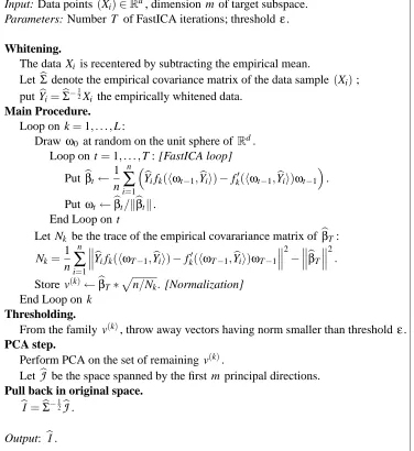
Input: Data points (Xi)∈Rd, dimension m of target subspace. Parameters: Number T of FastICA iterations; threshold ε.

Whitening.

The data Xi is recentered by subtracting the empirical mean.

LetΣb denote the empirical covariance matrix of the data sample (Xi);

putYbi=bΣ−

1

2X_i the empirically whitened data.

Main Procedure.

Loop on k=1, . . . ,L :

Draw ω0 at random on the unit sphere ofRd.

Loop on t=1, . . . ,T : [FastICA loop]

Put bβt ←

1

n n

∑

i=1

b

Yifk(_hωt₋1,Yibi)−fk0(hωt₋1,Yibi)ωt₋1

.

Put ωt←bβt/kbβtk.

End Loop on t

Let Nk be the trace of the empirical covarariance matrix of bβT:

Nk=

1

n n

∑

i=1

bYifk(hωT−1,Ybii)−fk0(hωT−1,Ybii)ωT−1

2−bβT

2.

Store v(k)_←bβT∗

p

n/Nk. [Normalization]

End Loop on k

Thresholding.

From the family v(k), throw away vectors having norm smaller than threshold ε.

PCA step.

Perform PCA on the set of remaining v(k).

Let

J

b be the space spanned by the first m principal directions.

Pull back in original space.

b

I

=bΣ−1 2

J

b.

Output: b

I

.

(14)

Analysis of the estimation error with exact whitening. We start by considering an idealized case where whitening is done using the true covariance matrix Σ: Y =Σ−12X .

In this case we have the following control of the estimation error:

Theorem 3 Let _{hk}Lk=1 be a family of smooth functions from Rd to R. Assume that

sup_y_,_kmax(_k∇hk(y)k,khk(y)k)<B and that X has covariance matrixΣ with

Σ−1_≤_K2_{, and is} such that for some λ0>0 the following inequality holds:

E[exp(λ0kXk)]≤a0<∞. (10)

Denote eh(y) =yh(y)₋∇h(y). Suppose X1, . . . ,Xn are i.i.d. copies of X and let Yi=Σ−12Xi. If we

define

b

βY(h) =

1

n n

∑

i=1

e

h(Yi) =

1

n n

∑

i=1

Yih(Yi)−∇h(Yi), (11)

and

b

σ2

Y(h) =

1

n n

∑

i=1

eh(Yi)−bβY(h)

2

, (12)

then for any δ<1

4, with probability at least 1−4δ the following bounds hold simultaneously for all k_{∈ {}1, . . . ,L_}:

dist

b

βY(hk),

J

≤2

r b

σ2

Y(hk)

log(Lδ−1_{) +}_{log d}

n +C

log(nLδ−1)log(Lδ−1)

n34

,

and

distΣ−12bβ_Y(h_k),

I

≤2K

r b

σ2

Y(hk)

log(Lδ−1_{) +}_{log d}

n +C

0

n34

,

where dist(γ,

I

) denotes the distance between a vector γ and the subspace

I

, and C,C0 are con-stants depending only on the parameters (d,λ0,a0,B,K).

Comments.

1. The above inequality tells us that the rate of convergence of the estimated vectors to the target

space is in this case of order n−1/2 (classical “parametric” rate). Furthermore, the theorem gives us an estimation of the relative size of the estimation error for different functions h through the empirical factor bσY(h) in the principal term of the bound. As announced in our

initial goals, this therefore gives a rigorous foundation to the intuition exposed in section 3.2 for vector renormalization.

2. Also following our goals, we obtained a uniform control of the estimation error over a finite

(15)

Whitening using empirical covariance. When Σ is unknown (which is in general the case), we use instead the empirical covariance matrixΣb. Here, we will show that, under a somewhat stronger assumption on the distribution of X and on the functions h , we are still able to obtain a convergence rate of order at most plog(n)/n towards the index space

I

.

Let us denoteYib=bΣ−12Xi the empirically whitened datapoints, eh(y) =yh(y)−∇h(y) as

previ-ously, and

b

βYb(h) =

1

n n

∑

i=1

e

h(Ybi) =

1

n n

∑

i=1

b

Yih(Ybi)−∇h(Ybi); (13)

finally, let us denote

bγ(h) =bΣ−12bβ b

Y(h), and bσ 2

b

Y(h) =

1

n n

∑

i=1

eh(Ybi)−bβYb(h)

2 .

We then have the following theorem:

Theorem 4 Let us assume the following : (i) There exists λ0>0,a0>0 such that

E

h

exp

λ0kXk2

i

=a0<∞;

(ii) The covariance matrix Σ of X is such that Σ−1_≤K2;

(iii) sup_k_,_ymax(_k∇hk(y)_k,_khk(y)_k)<B ;

(iv) The functions ehk(y) =∇hk(y)−yhk(y) are all Lipschitz with constant M. Then for big enough n , with probability at least 1−4

n−4δ the following bounds hold true simultaneously for all k_{∈ {}1, . . . ,L_}:

dist(bβ_Y_b(hk),

J

)≤C1

r

d log n n +2

r b

σ2

b

Y(hk)

log(Lδ−1_{) +}_{log d} n +C2

n34

,

and

dist(bγ(hk),

I

)_≤C₁0

r

d log n n +2K

r b

σ2

b

Y(hk)

log(Lδ−1_{) +}_{log d}

n +C

0 2

n34

,

where C1,C₁0 are constants depending on parameters (λ0,a0,B,K,M) only and C2,C0₂ on

(d,λ0,a0,B,K,M). Comments.

1. Theorem 4 implies that the vectors bγ(hk) obtained from any h(x) converge to the unknown

non-Gaussian subspace

I

uniformly at a rate of order plog(n)/n .

2. The condition (i) is a restrictive assumption as it excludes some densities with heavy tails. We

(16)

3. In the actual algorithm, we consider a family of functions of the form hω(x) = f(_hω,xi),

with ω on the unit sphere ofRd. Suppose we approximate ω by its nearest neighborωe on a regular grid of scale ε. Then we only have to apply the bound to a discretized family of size

L=

O

(ε1−d₎_{, giving rise only to an additional factor in the bound of order}p_{d log}ε₋1_{. Taking}

for example ε=1/n (the fact that the function family depends on n is not a problem since

the bounds are valid for any fixed n ), this ensures convergence of the discretized functions to the initial continuous family while introducing only in an additional factor √d log n in

the bound: this does not change fundamentally the order of the bound since there is already another √d log n term present.

4. For both Theorems 3 and 4, we have given bounds for estimation of both

I

and

J

, that is, in terms of the initial data and of the “whitened” data. The result in terms of the initial data ensures the overall consistency of the approach, but the convergence in the whitened space is equally interesting since we use it as the main working space for the algorithm and the bound itself is more precise.

5. Comparing to Theorem 3 obtained for exact whitening, we see in the present case that there

is an additional term of principal order in n coming from the estimation error of Σ, with a multiplicative factor which unfortunately is not known accurately. This means that the renormalization scheme is not completely justified in this case, although we feel the idealized situation of Theorem 3 already provides some strong argument in this direction. However, the present result suggests that the accuracy of the normalization could probably be further improved.

4. Numerical Results

We now turn to numerical evaluations of the NGCA method: first on simulated data, where the generating distribution is precisely known, then on exemplary, realistic data. All of the experiments

presented below, without exception, where obtained with exactly the same set of parameters: a_∈

[0,4]for the Fourier functions; b_∈[0,5]for the Hyperbolic Tangent functions; σ2_∈[0.5,5]for the Gauss-pow3 functions. Each of these ranges was divided into 1000 equispaced values, thus yielding a family _{fk}of size 4000 (Fourier functions count twice because of the sine and cosine parts). The

preliminary calibration procedure described in the end of section 3.2 suggested to take ε=1.5 as the threshold under which vectors are not informative (strictly speaking, the threshold should be calibrated separately for each function f but we opted here for a single threshold for simplicity). Finally we fixed the number of FastICA iterations T=10 . With this choice of parameters and 1000 data points in the sample, the computation time is typically of the order of less than 10 seconds on a modern PC under our Matlab implementation.

4.1 Tests in a Controlled Setting

(17)

(A) (B) (C) (D)

Figure 5: Densities of non-Gaussian components. The data sets are: (a) 2D independent Gaussian mixtures, (b) 2D isotropic super-Gaussian, (c) 2D isotropic uniform and (d) dependent 1D Laplacian + 1D uniform.

PP(pow3) PP(tanh) NGCA

0 0.5 1 1.5 2

2.5x 10

−3

PP(pow3) PP(tanh) NGCA

0 0.02 0.04 0.06 0.08 0.1 0.12 0.14 0.16

PP(pow3) PP(tanh) NGCA 0 0.005 0.01 0.015 0.02 0.025 0.03

(A) (B) (C) (D)

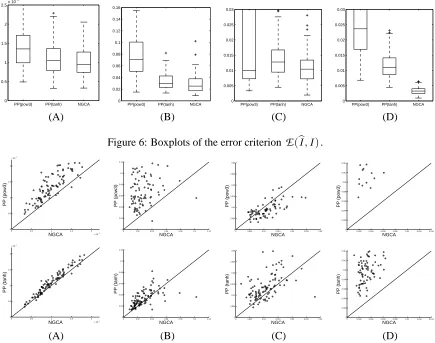
Figure 6: Boxplots of the error criterion

E

(b

I

,

I

).

0 0.5 1 1.5 2 x 10−3

NGCA

PP (pow3)

0 0.02 0.04 0.06 0.08 0.1 0.12 0 0.02 0.04 0.06 0.08 0.1 0.12 NGCA PP (pow3)

0 0.005 0.01 0.015 0.02 0.025 0.03 0 0.005 0.01 0.015 0.02 0.025 0.03 NGCA PP (pow3)

0 0.002 0.004 0.006 0.008 0.01 0.012 0.014 0 0.002 0.004 0.006 0.008 0.01 0.012 0.014 NGCA PP (pow3)

0 0.5 1 1.5 2 x 10−3

NGCA

PP (tanh)

0 0.02 0.04 0.06 0.08 0.1 0.12 0 0.02 0.04 0.06 0.08 0.1 0.12 NGCA PP (tanh)

0 0.005 0.01 0.015 0.02 0.025 0.03 0 0.005 0.01 0.015 0.02 0.025 0.03 NGCA PP (tanh)

0 0.002 0.004 0.006 0.008 0.01 0.012 0.014 0 0.002 0.004 0.006 0.008 0.01 0.012 0.014 NGCA PP (tanh)

(A) (B) (C) (D)

(18)

(A) Simple Gaussian Mixture: 2 -dimensional independent Gaussian mixtures, with the density

of each component given by

1

2φ−3,1(x) + 1

2φ3,1(x). (14)

(B) Dependent super-Gaussian: 2 -dimensional isotropic distribution with density proportional to

exp(_−kx_k).

(C) Dependent sub-Gaussian: 2 -dimensional isotropic uniform with constant positive density for

kx_{k ≤}1 and 0 otherwise.

(D) Dependent super- and sub-Gaussian: 1 -dimensional Laplacian with density proportional to

exp(_−|xLap|) and 1 -dimensional dependent uniform U(c,c+1), where c=0 for |xLap| ≤

log 2 and c=₋1 otherwise.

For each of these situations, the non-Gaussian components are additionally rescaled coordinatewise by a fixed factor so that each coordinate has unit variance. The profiles of the density functions of the non-Gaussian components in the above data sets are described in Figure 5.

We compare the following three methods in the experiments: PP with ‘pow3’ or ‘tanh’ index5

(denoted by PP(pow3) and PP(tanh), respectively), and the proposed NGCA.

Figure 6 shows boxplots of the error criterion

E

(b

I

,

I

) defined in Eq.(3) obtained from 100 runs. Figure 7 shows comparison of the errors obtained by different methods for each individual trial. Because PP tends to get trapped into local optima of the index function it optimizes, we restarted it 10 times with random starting points and took the subspace obtaining the best index value. However, even when it is restarted 10 times, PP (especially with the ‘pow3’ index) still gets caught in local optima in a small percentage of cases (we also tried up to 500 restarts but it led to negligible improvement).

For the simplest data set (A), NGCA is comparable or slightly better than PP methods. It is known that PP(tanh) is suitable for finding super-Gaussian components (heavy-tailed distribu-tion) while PP(pow3) is suitable for finding sub-Gaussian components (light-tailed distribudistribu-tion) (Hyv¨arinen et al., 2001). This can be observed in the data sets (B) and (C): PP(tanh) works well for the data set (B) and PP(pow3) works well for the data set (C), although the upper-quantile is very large for the data set (C) (because of PP getting trapped in local minima). The sample-wise plots of Figure 7 confirm that NGCA is on average on par with, or slightly better than, PP with the ‘correct’ non-Gaussianity index, without having to prefix such a non-Gaussianity index. For the data set (C), NGCA appears to be marginally worse than PP(pow3) (excluding those cases where PP fails due to local minima: the corresponding points are outside the range of the figure), but the difference appears hardly significant. The superiority of the index adaptation feature of NGCA can be clearly observed in the data set (D), which includes both sub- and super-Gaussian components. Because of this composition, there is no single best non-Gaussianity index for this data set, and the proposed NGCA gives significantly lower error than that of either PP method.

(19)

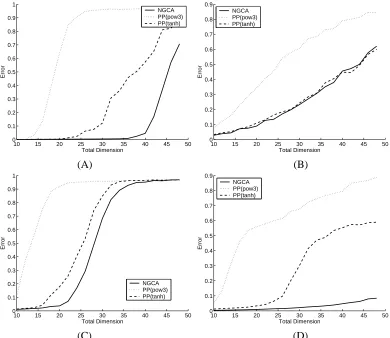
Failure modes. We now try to explore the limits of the method and the conditions under which estimation of the target space will fail. First, we study the behaviour of NGCA again compared with PP as the total dimension of the data increases. We use the same synthetic data sets with 2-dimensional non-Gaussian components, while the number of Gaussian components increases. The averaged errors over 100 experiments are depicted in Figure 8. In all cases, we seem to observe a sharp phase transition between a good behaviour regime and a failure mode where the procedure is unable to estimate the correct subspace. In 3 out of 4 cases, however, we observe that the phase transition to the failure mode occurs for a higher dimension for NGCA than for the PP methods, which indicates better robustness of NGCA.

10 15 20 25 30 35 40 45 50 0

0.1 0.2 0.3 0.4 0.5 0.6 0.7 0.8 0.9 1

Total Dimension

Error

NGCA PP(pow3) PP(tanh)

10 15 20 25 30 35 40 45 50 0

0.1 0.2 0.3 0.4 0.5 0.6 0.7 0.8 0.9

Total Dimension

Error

(A) (B)

10 15 20 25 30 35 40 45 50 0

0.1 0.2 0.3 0.4 0.5 0.6 0.7 0.8 0.9 1

Total Dimension

Error

10 15 20 25 30 35 40 45 50 0

0.1 0.2 0.3 0.4 0.5 0.6 0.7 0.8 0.9

Total Dimension

Error

(C) (D)

Figure 8: Results when the total dimension of the data increases.

In the synthetic data sets used so far, the data was always generated with a covariance matrix equal to identity. Another interesting setting to study is the robustness with respect to bad condi-tioning of the covariance matrix. We consider again a fixed-dimension setting, with 2 non-Gaussian and 8 gaussian dimensions.

(20)

0 0.5 1 1.5 2 0

0.05 0.1 0.15 0.2 0.25 0.3 0.35 0.4

Log

10 noise scaling range

Error

0 0.5 1 1.5 2 0

0.1 0.2 0.3 0.4 0.5 0.6 0.7 0.8 0.9

Log

Error

(A) (B)

0 0.5 1 1.5 2 0

0.1 0.2 0.3 0.4 0.5 0.6 0.7

Log

Error

0 0.5 1 1.5 2 0

0.1 0.2 0.3 0.4 0.5 0.6 0.7

Log

Error

(C) (D)

(21)

The results are depicted in Figure 9, where we observe again a transition to a failure mode when the covariance matrix is too badly conditioned. Although NGCA still appears as the best method, we observe that, on 3 out of 4 data sets, the transition to failure mode seems to happen roughly at the same point as for PP methods. This suggests that there is no or only little added robustness of NGCA with respect to PP in this regard. However, this result is not entirely surprising, as we expect this type of failure mode to be caused by a too large estimation error in the covariance matrix and therefore in the whitening/dewhitening steps. Since these steps are common to NGCA and the PP algorithms, it seems logical to expect a parallel evolution of their errors.

4.2 Example of Application for Realistic Data: Visualization and Clustering

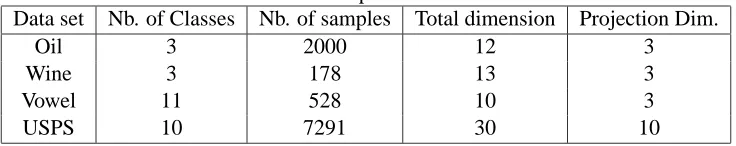
We now give an example of application of our methodology to visualization and clustering of real-istic data. We consider here “oil flow” data, which has been obtained by numerical simulation of a complex physical model. This data was already used before for testing techniques of dimension reduction (Bishop et al., 1998). The data is 12-dimensional and it is not known a priori if some dimensions are more relevant. Here our goal is to visualize the data and possibly exhibit a clustered structure. Furthermore, it is known that the data is divided into 3 classes. We show classes with different marker types but the class information is not used in finding the directions (i.e., the process is unsupervised).

We compare the NGCA methodology described in the previous section, projection pursuit (“vanilla” FastICA) using the tanh or the pow3 index, and Isomap (non-linear projection method, see Tenenbaum et al., 2000). The results are shown on Figure 10. A 3D projection of the data was computed using these methods, which was in turn projected in 2D to draw the figure; this last projection was chosen manually so as to make the cluster structure as visible as possible in each case.

We see that the NGCA methodology gives a much more relevant projection than PP using either tanh or pow3 alone: we can distinguish 10-11 clusters versus at most 5 for the PP methods and 7-8 for Isomap. Furthermore, the classes are clearly separated only on the NGCA projection; on the other ones, they are partially confounded in one single cluster. Finally, we confirm, by applying the projection found to held-out test data (i.e., data not used to determine the projection), that the cluster structure is relevant and not due to some overfitting artifact. This, in passing, shows one advantage of a linear projection method, namely that it can be extended to new data in a straightforward way.

(22)

FastICA, tanh index FastICA, pow3 index

NGCA (training data) NGCA (held-out test data)

NGCA without Fourier functions Isomap

(23)

NGCA is combining indices (as well as combining over the parameters ranges σ2 and b ). This is confirmed in Figure 10: even without the relevant Fourier functions, NGCA yields a projection where 8 clusters can be distinguished, and the classes are much more clearly separated than with PP methods. Finally, a visual comparison with the results obtained by Bishop et al. (1998) demonstrated that the projection found by our algorithm exhibits a clearer clustered structure; moreover, ours is a purely linear projection whereas the latter reference was a nonlinear data representation

Further analysis on clustering performance with additional data sets are given in the Appendix and underline the usefulness of our method.

5. Conclusion

We proposed a new semi-parametric framework for constructing a linear projection to separate an uninteresting multivariate Gaussian ‘noise’ subspace of possibly large amplitude from the ‘signal-of-interest’ subspace. Our theory provides generic consistency results on how well the non-Gaussian directions can be identified (Theorem 4). To estimate the non-Gaussian subspace from the set of vectors obtained, PCA is finally performed after suitable renormalization and elimination of uninfor-mative vectors. The key ingredient of our NGCA method is to make use of the gradient computed for the nonlinear basis function h(x) in Eq.(11) after data whitening. Once the low-dimensional ‘signal’ part is extracted, we can use it for a variety of applications such as data visualization, clus-tering, denoising or classification.

Numerically, we found comparable or superior performance to, e.g., FastICA in deflation mode as a generic representative of the family of PP algorithms. Note that, in general, PP methods need to pre-specify a projection index used to search for non-Gaussian components. By contrast, an important advantage of our method is that we are able to simultaneously use several families of nonlinear functions; moreover, inside a same function family, we are able to use an entire range of parameters (such as frequency for Fourier functions). Thus, our new method provides higher flexibility, and less restricting assumptions a priori on the data. In a sense, the functional indices that are the most relevant for the data at hand are automatically selected.

Future research will adapt the theory to simultaneously estimate the dimension of the non-Gaussian subspace. Extending the proposed framework to non-linear projection scenarios (Cox and Cox, 1994; Sch¨olkopf et al., 1998; Roweis and Saul, 2000; Tenenbaum et al., 2000; Belkin and Niyogi, 2003; Harmeling et al., 2003) and to finding the most discriminative directions using labels are examples for which the current theory could be taken as a basis.

(24)

Appendix A. Proofs of the Theorems

A.1 Proof of Lemma 1

Suppose first that the noise N is standard normal. Denote by ΠE the projector from Rd to Rm

which corresponds to the subspace E . Let also E⊥ be the subspace complementary to E and Π_E⊥

mean the projector on E⊥. The standard normal noise can be decomposed as N=N1uN2 where

N1=ΠEN and N2 =Π_E⊥N are independent noise components. Similarly, the signal X can be decomposed as

X= (ΠES+N1)uN2

where we have used the model assumption that the signal S is concentrated in E and it is inde-pendent of N . It is clear that the density of ΠES+N1 in Rm can be represented as the product g(x1)φ(x1) for some function g and the standard normal density φ(x1), x1∈Rm. The

indepen-dence of N1 and N2 yields the in the similar way for x= (x1,x2) with x1=ΠEx and x2=ΠE⊥x that p(x) =g(x1)φ(x1)φ(x2) =g(x1)φ(x). Note that for the linear mapping T =ΠE characterizes

the signal subspace E . Namely, E is the image ℑ(T∗) of the dual operator T∗ while E⊥ is the null subspace (kernel) of T : E⊥=K(T).

Next we drop the assumption of the standard normal noise and assume only that the covariance

matrix Γ of the noise is nondegenerated. Multiplying the both sides of the equation (1) by

the matrix Γ−1/2 _{leads to} Γ−1/2_X ₌Γ−1/2_S₊_{N where}_e _N_e ₌Γ−1/2_{N is standard normal. The}

transformed signal Xe=Γ−1/2_{S belongs to the subspace} _E_e₌Γ−1/2_{E . Therefore, the density}

of X can be represented as pe (xe) =eg(Π_E_exe)φ(xe) where Π_E_e is the projector corresponding to E .e

Coming back the variable x yields the density of X in the form p(x) =g(T x)φ(Γ−1/2_x₎ _where T =Π_E_eΓ−1/2_.

A.2 Proof of Proposition 2

For any functionψ(x), it holds that

Z

ψ(x+u)p(x)dx=

Z

ψ(x)p(x₋u)dx,

if the integrals exists. Under mild regularity conditions on p(x) and ψ(x) allowing differentiation under the integral sign, differentiating this with respect to u gives

Z

∇ψ(x)p(x)dx=₋

Z

ψ(x)∇p(x)dx. (15)

Let us take the following function

ψh(x):=h(x)−x>E[X h(X)],

whose gradient is

∇ψh(x) =∇h(x)−E[X h(X)].

The vectorβ(h) is the expectation of −∇ψh. From Eq.(15) and using ∇p(x) =∇log p(x)p(x), we

have

β(h) =

Z

(25)

Applying Eq.(2) to the above equation yields

β(h) =

Z

ψh(x)∇log g(T x) p(x)dx−

Z

ψh(x)Γ−1x p(x)dx

= T∗

Z

ψh(x)∇g(T x)φθ,Γ(x)dx−Γ−1

Z

xψh(x)p(x)dx. (16)

Under the assumption EX X>=Id, we get

E[Xψh(X)] =E[X h(X)]−E

h

X X>

i

E[X h(X)] =0,

that is, the second term of Eq.(16) vanishes. Since the first term of Eq.(16) belongs to

I

by the definition of

I

, we finally have β(h)_∈

I

.

A.3 Proof of Theorem 3

For a fixed function h, we will essentially apply Lemma 5 stated below for each coordinate ofβY(h).

Denoting the k -th coordinate of a vector v by v(k), and y=Σ−12x , we have

eh(k)(x) =

[∇h(y)₋yh(y)](k)

≤B(1+_ky_k)_≤B(1+K_kx_k).

It follows that eh(k)(x) is such that

E

exp

_λ

0 BKeh

(k)₍_x₎

≤a0exp

_λ

0 K

,

and hence satisfies the assumption of Lemma 5. Denoting by bσ2

k the sample variance of eh(k), we

apply the lemma with δ0=δ/d , obtaining by the union bound that with probability at least 1₋4δ, for all 1_≤k_≤d :

h

βY−bβY

i(k)2

≤4bσ2 k

log dδ−1

n +C1(λ0,a0,B,d,K)

log2(nδ−1)log2δ−1

n32

,

where we have used the inequality(a+b)2_≤₂₍_a2₊_b2₎_{, and C}

1 denotes some function depending

only on the indicated quantities. Now summing over the coordinates, taking the square root and using √a+b_≤√a+√b leads to:

βY−bβY

≤2

r b

σ2

Y(h)

logδ−1₊_{log d}

n +C2(λ0,a0,B,d,K)

log(nδ−1)logδ−1

n34

, (17)

with probability at least 1₋4δ. To turn this into a uniform bound over the family_{hk}Lk=1, we

simply apply this inequality separately to each function in the family withδ00=δ/L. This leads to

the first announced inequality of theorem. We obtain the second one by multiplying the first by

Σ−1

(26)

Lemma 5 Let X be a real random variable such that for someλ0>0 : E[exp(λ0|X|)]≤a0<∞.

Let X1, . . . ,Xn denote an i.i.d. sequence of copies of X . Let µ=E[X], bµ= 1_n∑n_i₌₁Xi and σb2₌ 1

2n(n−1)∑i6=j(Xi−Xj)2 be the sample variance.

Then for any δ<1₄ the following holds with probability at least 1₋4δ, where c is a universal constant:

|µ₋_bµ_{| ≤}

r

2bσ2_logδ−1 n +cλ

−1

0 max 1,log na0δ−1

logδ−1

n

3 4

+logδ−

1 n

!

.

Proof For A>0 denote XA=X 1_{|X_{| ≤}A_}. We decompose

1 n n

∑

i=1 Xi−µ

≤ 1 n n

∑

i=1

Xi−XiA

+ 1 n n

∑

i=1

X_iA₋EXA

+

_EX₋XA;

these three terms will be denoted by T1,T2,T3. By Markov’s inequality, it holds that

P[_|X_|>t]_≤a0exp(−λ0t),

Fixing A=log nδ−1a0

/λ0 for the rest of the proof, it follows by taking t =A in the above

inequality that for any 1_≤i_≤n :

PX_iA₆=Xi_≤δ n.

By the union bound, we then have X_iA=Xi for all i , and therefore T1=0 , except for a set ΩA of

probability bounded by δ.

We now deal with the third term: we have

T3=_|E[X 1_{|X_|>A_}]_{| ≤}E[X 1_{X >A_}] =

Z ∞

0 P

[X 1_{X>A_}>t]dt

≤AP[X>A] +

Z ∞

A

a0exp(₋λ0t)dt

≤a0 A+λ−01

exp(₋λ0A)

= δ

nλ0

1+log nδ−1a0.

Finally, for the second term, since XA_≤A=λ−₀1log nδ−1a0

, Bernstein’s inequality ensures that with probability as least 1₋2δ the following holds:

1 n n

∑

i=1

X_iA₋EXA

≤ r

2Var[XA_]_logδ−1

n +2

log nδ−1a0

logδ−1

λ0n .

We finally turn to the estimation of VarXA. The sample variance of XA is given by

(bσA₎2₌ 1

2n(n₋1)

∑

_i₆₌_j X

A i −XAj

(27)

Note that (bσA₎2 _{is an unbiased estimator of Var}_XA_{. Furthermore, replacing X}A

i by Xi0A in the

above expression changes this quantity at most of 4A2/n since XA

i appears only in 2(n−1) terms.

Therefore, application of the bounded difference (a.k.a. McDiarmid’s) inequality (McDiarmid , 1989) to the random variableσbA _{yields that with probability 1}₋δ _{we have}

(σbA₎2₋_Var_XA_≤_4A2

r

logδ−1 n ;

finally, except for samples in the set ΩA which we have already excluded above, we have bσA=σb.

Gathering these inequalities lead to the conclusion.

A.4 Proof of Theorem 4

In this proof we will denote by C(_·) a factor depending only on the quantities inside the parentheses, and whose exact value can vary from line to line.

From Lemmas 9 and 10 below, we conclude that for big enough n , the following inequality is satisfied with probability 1₋2/n:

Σ−12−Σb−12

≤C(a0,λ0,K)

r

d log n

n ; (18)

also, it is a a weaker consequence of Lemmas 7 and 8 that the following inequalities hold with probability at least 1−1/n each (again for n big enough):

1

n n

∑

i=1

kXik ≤C(a0,λ0), (19)

1

n n

∑

i=1

kXik2≤C(a0,λ0). (20)

Let us denoteΩthe set of samples where (18), (19) and (20) are satisfied simultaneously; from the above, we conclude that for large enough n , the setΩcontains the sample with probability at least 1₋4/n. For the remainder of the proof, we suppose that this condition is satisfied.

For any function h, we have

bβYb−βY

≤bβYb−bβY

+_bβY−βY

.

Note that (up to some changes in the constants) the assumption on the Laplace transform is stronger than the assumption of Theorem 3; hence equation (17) in the proof of this theorem holds and we have with probability at least 1₋4δ, for any function in the family_{hk}Lk=1:

βY−bβY

≤2

r b

σ2

Y(h)

log(Lδ−1_{) +}_{log d}

n +C(λ0,a0,B,d,K)

log(nLδ−1)log Lδ−1

n34

!