Bayesian Learning in Sparse Graphical Factor Models via Variational Mean-Field Annealing

(1)

Bayesian Learning in Sparse Graphical Factor Models via

Variational Mean-Field Annealing

Ryo Yoshida [email protected]

Department of Statistical Modeling Institute of Statistical Mathematics Tachikawa, Tokyo 190-8562, Japan

Mike West [email protected]

Department of Statistical Science Duke University

Durham, NC 27708-0251, USA

Editor: Michael Jordan

Abstract

We describe a class of sparse latent factor models, called graphical factor models (GFMs), and relevant sparse learning algorithms for posterior mode estimation. Linear, Gaussian GFMs have

sparse, orthogonal factor loadings matrices, that, in addition to sparsity of the implied covariance

matrices, also induce conditional independence structures via zeros in the implied precision ma-trices. We describe the models and their use for robust estimation of sparse latent factor structure and data/signal reconstruction. We develop computational algorithms for model exploration and posterior mode search, addressing the hard combinatorial optimization involved in the search over a huge space of potential sparse configurations. A mean-field variational technique coupled with annealing is developed to successively generate “artificial” posterior distributions that, at the limit-ing temperature in the anneallimit-ing schedule, define required posterior modes in the GFM parameter space. Several detailed empirical studies and comparisons to related approaches are discussed, including analyses of handwritten digit image and cancer gene expression data.

Keywords: annealing, graphical factor models, variational mean-field method, MAP estimation,

sparse factor analysis, gene expression profiling

1. Introduction

(2)

compu-tational technique for posterior mode evaluation using a hybrid of variational mean-field method (Attias, 1999; Wainwright and Jordan, 2008) and annealing-based optimization.

As a previously unexplored class of sparse (linear, Gaussian) factor models, the intrinsic graph-ical structure of the GFM arises from use of an orthogonal factor loadings matrix and appropriate scaling of its columns, together with the usual diagonal covariance matrix for latent factors (with no loss of generality). We show that this generally induces zero elements in the precision matrix of the GFM, as well as the covariance matrix. Particularly, the zero entries in the covariance matrix have corresponding zeros in the precision matrix. We also show that covariance matrices of fitted values (i.e., “data reconstructions”) from such a model have the same sparse structure, and demonstrate aspects of robustness of the model in inferring variable-latent factor relationships in the presence of outliers. These properties are not shared in general by sparse factor models that lack the graph-ical structure on variables, nor of course by non-sparse approaches. These intrinsic properties of the GFM, along with relationships with earlier studies on sparse factor analyses, are discussed in Section 2.

Our variational mean-field annealing algorithm (VMA2) addresses the combinatorial optimiza-tion involved in aiming to compute approximate posterior modes for GFM parameters in the context of the huge space of zero/non-zero potential patterns in factor loadings. Using a prescribed schedule of decreasing temperatures, VMA2 successively generates tempered “artificial” posteriors that, at the limiting zero temperature, yield posterior modes for both GFM parameters and the 0/1 loadings indicators. Defined via an artificial, dynamic regularization on the posterior entropy of configured sparse structures, VMA2 is developed in Section 3.

Section 4 provides additional algorithmic details, including prior modelling for evaluating de-gree of sparseness, and a stochastic variant of VMA2 for higher-dimensional problems is described in Section 5. Performance and comparisons on artificial data appear in Section 6. Section 7 summa-rizes extensive, detailed empirical comparisons with related approaches in analyses of hand-written digit images and cancer gene expression data. Section 8 concludes with brief additional comments. A range of detailed supplementary materials, extended discussion on the gene expression studies

andRcode, is accessible fromhttp://daweb.ism.ac.jp/˜yoshidar/anneals/.

2. Sparse Graphical Factor Models

We describe the GFM with some intrinsic graphical properties, followed by connections to previ-ously developed classes of sparse latent factor analyses.

2.1 GFM Form

Observed sample vectors xi∈Rp in p dimensional feature space are each linearly related to

in-dependent, unobserved Gaussian latent factor vectorsλi∈Rk with additional Gaussian noise. We

are interested in sparse variable-factor relationships so that the bipartite mappingλ→x is sparse,

with the underlying p×k matrix of coefficients—the factor loadings matrix—having a number of

zero elements; the p×k binary matrix Z defines this configured sparsity pattern. We use a sparse,

(3)

With Z as the p×k binary matrix with elements zg j such that variable g is related to factor j if and only if zg j=1,the GFM is

xi=Ψ1/2ΦZλi+νi with λi∼

N

(λi|0,∆) and νi∼

N

(νi|0,Ψ)

where: (a) the factor loading matrix Ψ1/2ΦZ has ΦZ ≡Φ◦Z with ◦ representing element-wise

product; (b)ΦZ is orthogonal, that is,Φ′ZΦZ=Ik; (c) the factors have diagonal covariance matrix

∆=diag(δ1, . . . ,δk); and (d) the idiosyncratic Gaussian noise (or residual)νi is independent ofλi and has covariance matrixΨ=diag(ψ1, . . . ,ψp).The implied covariance matrix of the sampling model,Σ,and the corresponding precision matrix,Σ−1,are

Σ=Ψ1/2{I+ΦZ∆Φ′Z}Ψ1/2 and Σ−1=Ψ−1/2{I−ΦZTΦ′Z}Ψ−1/2 (1) where T =diag(τ1, . . . ,τk)with τj =δj/(1+δj) (j=1 : k).In general, sparse loading matrices induce some zero elements in the covariance matrix whether or not they are orthogonal, but not in the implied precision matrix. In the GFM here, however, a sparse factor model also induces off-diagonal zeros inΣ−1.Zeros in the precision matrix defines a conditional independence or graphical model, hence the GFM terminology. In (1), the pattern of sparsity (location of zero entries) in the covariance and precision matrices are the same. The set of variables associated with one specific factor forms a clique in the induced graphical model, with sets of variables that have non-zero loadings on any two factors lying in the separating subgraph between the corresponding cliques. Hence, we have a natural and appealing framework in which sparse factor models and graphical models are reconciled and consistent.

2.2 Some Model Attributes

In general, a non-orthogonal factor model with the sparse loading matrix W —a sparse extension of probabilistic PCA (Bishop, 1999, 2006)—has the form

xi=Wλi+νi withλi∼N(0,I)andνi∼N(0,Ψ).

The GFM arises when a singular value decomposition is applied to the scaled-factor loading matrix

Ψ−1/2_W ₌_Φ

Z∆1/2R with a k×k orthogonal matrix R being removed. This non-orthogonal model defines a Bayes optimal reconstruction of the data via the fitted values (or extracted signal)

ˆx(xi):=WE[λi|xi] =WW′(WW′+Ψ)−1xi.

Then, asymptotically,

1

n

∑

i=1

ˆx(xi)ˆx(xi)′ p

−→C_ov_[ˆx(_x_i_{)] =}_WW′₍_WW′₊Ψ₎−1_WW′

and this is generally a non-sparse matrix (no zero entries) even though W is sparse. This is an incon-sistency in the sense that data reconstructions should be expected to share the dominant patterns of covariance sparsity evident in the original covariance matrixC_ov_[_x_i_{] =}_WW′₊Ψ._{In the GFM,}

how-ever,C_ov_[ˆx(_x_i_{)] =}Ψ1/2Φ_Z_GΦ′_ZΨ1/2 _{where G is diagonal with entries}δ2

j/(1+δj). In such cases,

C_ov_[ˆx(_x_i_)]_{is sparse and shares the same 0 elements as}C_ov_[_x_i_]_.

(4)

x

1

x

2

x

3

x

4

λ₁ λ₂

x

1

x

2

x

3

x

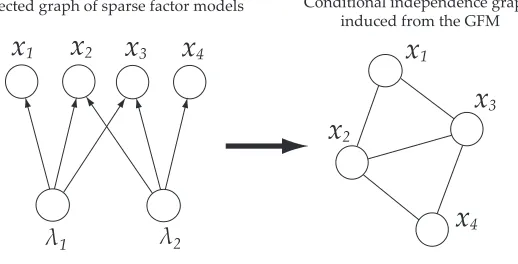
4

Directed graph of sparse factor models Conditional independence graph induced from the GFM

Figure 1: Graphical model structure of an example GFM.

with two cliques in the conditional independence graph; {xi1,xi2,xi3} ←λi1 and{xi2,xi3,xi4} ←

λi2 (see Figure 1). The graph defines the decomposition of the joint density p(xi1,xi2,xi3,xi4) =

p(xi1|xi2,xi3)p(xi2,xi3|xi4)p(xi4) or p(xi1,xi2,xi3,xi4) =p(xi4|xi2,xi3)p(xi2,xi3|xi1)p(xi1). This im-plies that presence of one or more outliers in the isolated feature variable, that is, xi1 or xi4, asso-ciated with a single factor clique, has no effect on the variables, xi4 or xi1, once the intermediate variables xi2 and xi3 are given. Then, the parameters involved in p(xi1) or p(xi4), for instance, the loading components and the noise variances corresponding to the isolated variable, can be estimated independently of the impact of outliers in xi4or xi1. The numerical experiment shown in Section 7.1 highlights this robustness property in terms of data compression/restoration tasks, with comparison to other sparse factor models.

2.3 Likelihood, Priors and Posterior

Denote by Θ the full set of parametersΘ={Φ,∆,Ψ}. Our computations aim to explore model

structures Z and corresponding posterior modes of parameters Θ under the posterior p(Z,Θ|X)

using specified priors and based on the n observations forming the columns of the p×n data matrix X .

2.3.1 LIKELIHOOD FUNCTION

The likelihood function is

p(X|Z,Θ)∝|Ψ|−n/2_|_I₋_T_|n/2_etr(₋_S_Ψ−1_/₂₊_Ψ−1/2_S_Ψ−1/2_Φ

ZTΦ′Z/2) (2)

where etr(A) =exp(trace(A))for any square matrix A,and S is the sample sum-of-square matrix

S=X X′ with elements sgh. In (2), the factor loadings appear only in the last term and form the important statistic

trace(Ψ−1/2SΨ−1/2ΦZTΦ′Z) = k

∑

j=1

τjφ′z jΨ−1/2SΨ−1/2φz j

(5)

2.3.2 PRIORS ONΘANDZ

Priors over non-zero factor loadings may reflect substantive a priori knowledge if available, and will then be inherently context specific. For examples here, however, we use uniform priors p(Θ|Z)

for exposition. Note that, on the critical factor loadings elements Φ, this involves a uniform on

the hypersphere defined by the orthogonality constraint that is then simply conditioned (by setting

implied elements ofΦto zero) as we move across candidate models Z.

Concerning the sparse structure Z,we adopt independent priors on the binary variates zg j with logit(Pr(zg j=1|ζg j)) =−ζg j/2 where logit(p) =log(p/(1−p))and the parametersζg j are as-signed hyperpriors and included in the overall parameter set in later. Beta priors are obvious al-ternatives to this; the logit leads to a minor algorithmic simplification, but otherwise the choice is arbitrary. Using beta priors can be expected to lead to modest differences, if any of practical relevance, in many cases, and users are free to explore variants. The critical point is that includ-ing Bayesian inference on these p×k sparsity-determining quantities leads to “self-organization” as

their posterior distributions concentrate on larger or smaller values. Examples in Section 6 highlight this.

2.4 MAP Estimation for(Θ,Z)in GFMs

Conditional on the p×k matrix of sparsity control hyperparametersζwhose elements are theζg j, it follows that posterior modes(Z,Θ)maximize

2 log p(Z,Θ|X,ζ) = 2 log p(Θ|Z)− p

∑

g=1

k

∑

j=1

zg jζg j− p

∑

g=1

(n logψg+sggψ−1g )

+ k

∑

j=1

(n log(1−τj) +τjφz j′ Ψ−1/2SΨ−1/2φz j). (3)

The first two terms in (3) arise from the specified priors forΘand Z, respectively. The quadratic form in the last term isφ′_{z j}Ψ−1/2SΨ−1/2φ_{z j}=φ′_jS(zj,Ψ)φjfor each j,where the key p×p matrices

S(zj,Ψ)have elements(S(zj,Ψ))_ghgiven by

(S(zj,Ψ))gh=zg jzh jsgh(ψgψh)−1/2, for g,h=1 : p. (4)

The (relative) signal-to-noise ratiosτj=δj/(1+δj)control the roles played by the last term in (3).

Optimizing (3) over Θ and Z involves many discrete variables and the consequent

combina-torial computational challenge. Greedy hill-climbing approaches will get stuck at improper local solutions, often and quickly. The VMA2 method in Section 3 addresses this.

2.5 Links to Previous Sparse Factor Modelling and Learning

In the MAP estimation defined by (3), there are evident connections with traditional sparse princi-pal component analyses (sparse PCA; Jolliffe et al., 2003, Zou et al., 2006 and d’Aspremont et al.,

2007). IfΨ=I and ∆=I,the latter likelihood component in (3) is the pooled-variance of

(6)

The direct sparse PCA of d’Aspremont et al. (2007) imposes an upper-bound d >0 on the

cardinality of zj (the number of non-zero elements), with a resulting semidefinite programming of

computational complexity O(p4plog(p)).The applicability of that approach is therefore limited to problems with p rather small. Such cardinality constraints can be regarded as suggestive of structure for the prior distribution onζin our model.

The SCoTLASS algorithm of Jolliffe et al. (2003) uses ℓ1-regularization on loading vectors,

later extended to SPCA using elastic nets by Zou et al. (2006). Recently, Mairal et al. (2009)

presented a ℓ1-based dictionary learning for sparse coding in which the method aims to explore

sparsity on factor-sample mapping rather than that on factor-variable relations. Setting Laplace-like prior distributions on scale loadings is a counterpart ofℓ1-based penalization (Jolliffe et al., 2003;

Zou et al., 2006). However, our model-based perspective aims for a more probabilistic analysis, with advantages in probabilistic assessment of appropriate dimension of the latent factor space as well as flexibility in the determination of effective degrees of sparseness via the additional parameters

ζ.Other than the preceding studies,ℓ1-regularizations have widely been employed to make sparse

latent factor analyses. Archambeau and Bach (2009) developed a general class of sparse latent factor analyses involving sparse probabilistic PCA (Guan and Dy, 2009) and a sparse variant of probabilistic canonical correlation analysis. A key idea of Archambeau and Bach (2009) is to place the automatic relevance determination (ARD) prior of Mackay (1995) on each loading component, and to apply a variational mean-field learning method.

Key advances in Bayesian sparse factor analysis build on non-parametric Bayesian modelling in Griffiths and Ghahramani (2006) and Rai and Daum´e (2009), and developments in Carvalho et al. (2008) stemming from the original sparse Bayesian models in West (2003). Carvalho et al develop MCMC and stochastic search methods for posterior exploration. MCMC posterior sampling can be effective but is hugely challenged as the dimensions of data and factor variables increase. Our focus here is MAP evaluation with a view to scaling to increasingly large dimensions, and we leave open the opportunities for future work on MCMC methods in GFMs.

Most importantly, as remarked in Section 2.2, the GFM differs from some of the forgoing mod-els in the conditional independence graphical structures induced. This characteristic contributes to preserving sparse structure in the data compression/reconstruction process and also to the outlier robustness issue. We leave further comparative discussion to Section 7.1, where we evaluate some of the foregoing methods relative to the sparse GFM analysis in an image processing study.

3. Variational Mean-Field Annealing for MAP Search

Finding MAP estimates of the augmented posterior distribution (3) involves many discrete variables

zg j. Then, commonly applied search methods such as greedy hill-climbing algorithm often get stuck in improper local solutions. Here, we present a general framework of VMA2 enabling us to escape local mode traps by exploiting annealing.

3.1 Basic Principle

Relative to (3), consider the class of extended objective functions

G

T(Θ,ω) =

∑

Z∈Z

ω(Z)log p(X,Z,Θ|ζ)−T

∑

Z∈Z

(7)

whereω(Z)—the sparsity configuration probability—represents any distribution over Z∈Z _that

may depend on(X,Θ,ζ), and where T≥0.This modifies the original criterion (3) by taking the expectation of p(X,Z,Θ|ζ)with respect toω(Z)—the expected complete data log-likelihood in the

context of EM algorithm—and by the inclusion of Shannon’s entropy ofω(Z)with the temperature

multiplier T.

Now, view (5) as a criterion to maximize over(Θ,ω)jointly for any given T.The following is a key result:

Proposition 1 For any given parametersΘand temperature T , (5) is maximized with respect toω at

ωT(Z)∝p(Z|X,Θ,ζ)1/T. (6)

Proof See the Appendix.

For any givenΘ,a large T leads toωT(Z)being rather diffuse over sparse configurations Z so that

iterative optimization—alternating between Θ andω—will tend to move more easily and freely

around the high-dimensional space Z.This suggests annealing beginning with the temperature T

large and successively reducing towards zero. We note that:

• As T →0,ωT(Z) converges to a distribution degenerate at the conditional mode ˆZ(Θ,ζ)of

p(Z|X,Θ,ζ),so that

• joint maximization of

G

T(Θ,ω)would approach the global maximum of the exact posterior

p(Θ,Z|X,ζ)as T →0.

The notion of the annealing operation is to realize a gradual move of successively-generated solu-tions forΘandωT(Z), and to escape local mode traps by exploiting annealing. Note that, for any given tempered posterior (6), the expectation in the first term of (5) is virtually impossible to be taken due to the combinatorial explosion. In what follows, we introduce VMA2 as a mean-field technique coupled with the annealing-based optimization to overcome this central computational difficulty.

3.2 VMA2 based on Factorized, Tempered Posteriors

To define and implement a specific algorithm, we constrain the otherwise arbitrary “artificial

con-figuration probabilities”ω,and do so using a construction that induces analytic tractability. We specify the simplest, factorized form

ω(Z) = p

∏

g=1

k

∏

j=1

ω(zg j):= p

∏

g=1

k

∏

j=1 ωzg j

g j(1−ωg j)1−zg j

in the same way as conventional Variational Bayes (VB) procedures do. In this GFM context, the resulting optimization is eased using this independence relaxation as it gives rise to tractability in computing the conditional expectation in the first term of (5).

If T =1, and given the factorized ω, the objective function

G1

exactly agrees with the free

energy, which bounds the posterior marginal as

log

∑

Z∈Z

(8)

The lower-bound

G1

is the criterion that the conventional VB methods aim to maximize (Wainwright and Jordan, 2008). This indicates that any solutions corresponding to the VB inference can be

obtained by stopping the cooling schedule at T =1 in our method. Similar ideas have, of course,

6=g

∏

l6=j

ω(zhl)log

p(zg j=1,X,ZC\{g,j},Θ,ζ) p(zg j=0,X,ZC\{g,j},Θ,ζ)

>0,

0, otherwise.

It remains true that, at the limiting zero temperature, the global maximum of

G

T(Θ,ω)is the set of p×k point masses at the global posterior mode of p(Θ,Z|X,ζ). This is seen trivially as follows:

(i) As T →0, and with the non-factorizedωin (5), we have limiting value

sup Z

log p(X,Θ,Z|ζ) =sup

ω

G0

(Θ,ω) (8)

with the point mass ω(Z) =δZˆ(Z) at the location of the global maximum(Zˆ)g j = ˆzg j. Further,

(ii) any point mass δ_Zˆ(Z) is representable by a fully factorized p×k point masses as δ_Zˆ(Z) = ∏g,jδˆzg j(zg j).

It is stressed that the coordinate-basis updates (7) cannot, of course, guarantee convergence to the global optimum even with prescribed annealing. Nevertheless, VMA2 represents a substantial advance in its ability to move more freely and escape local mode traps. We also note the generality of the idea, beyond factor models and also potentially using penalty functions other than entropy.

4. Sparse Learning in Graphical Factor Models

We first provide a specific form of VMA2 for the GFM, and then address the issue of evaluating relevant degrees of sparseness.

4.1 MAP Algorithm

Computations alternate between conditional maximization steps for ω andΘ while reducing the

(9)

1: Set a cooling schedule

T

={T1, . . . ,Td}of length d where Td=0;

2: Setζ;

3: InitializeΘ;

4: Initializeω(Z);

5: i←0;

6: while({the loop is not converged}∧{i≤d})

7: i←i+1;

8: Compute configuration probabilitiesωg j(Ti);

9: Optimize with respect to each column φ_j (j=1 : k) of Φ in turn under

full-conditioning;

10: Optimize with respect to∆under full-conditioning;

11: Optimize with respect toΨunder full-conditioning;

12: Optimize with respect toζunder full-conditioning;

13: end while

We now summarize key components in the iterative, annealed computation defined above.

4.2 Sparse Configuration Probabilities

First consider maximization with respect to each sparse configuration probabilityωg j conditional on all others. We note that the first term in (5) involves the expectation over Z with respect to the probabilitiesω,denoted byEω_[_·_]_._{Accordingly, for the key terms S(}_z_j_,Ψ₎_{we have}

Eω_[_S₍_z_j,Ψ_{)] =}Ω_j_◦₍Ψ−1/2_SΨ−1/2₎_with₍Ω_j₎_gh₌

(

ωg j, if g=h,

ωg jωh j, otherwise.

(9)

Introduce the notationΨ−1/2SΨ−1/2= (s1(Ψ), . . . ,sp(Ψ))to represent the p columns of the

scaled-sample sum-of-square matrix here, and define the p−vector

˜

ωg j= (ω1 j, . . . ,ωg−1,j,1,ωg+1,j, . . . ,ωp j)′.

Then, the partial derivative of (5) with respect toωg j conditional onΘand the other configuration probabilities leads to

logit(ωg j(T)) =Hg j(ζg j)/T where Hg j(ζg j):=τjφg j(φj◦ω˜g j)′sg(Ψ)−ζg j.

This directly yields the conditional maximizer for ωg j in terms of the tempered negative energy

Hg j(ζg j)/T . As the temperature T is reduced towards zero, the resulting estimate tends towards 0 or 1 according to the sign of Hg j(ζg j).

4.3 Conditional Optimization overΦ

The terms in (5) that involve Φare simply the expectation of the quadratic forms in the last term

(10)

values of all other columns. In the context of the overall iterative MAP algorithm, this yields global

optimization overΦas T →0.

Conditional optimization then reduces to the following: for each j=1 : k,sequence through

each columnφ_jin turn and at each step

maximize

φj

φ′

jEω[S(zj,Ψ)]φj

subject to φ′_jφ_j=1 and φ′_mφ_j=0 for m6= j,m=1 : k. (10)

The optimization conditions on the most recently updated values of all other columns m6= j at each

step, and is performed as one sweep as the line9in the algorithm of Section 4.1. Column order can be chosen randomly or systematically each time while still maintaining convergence. In this step, we stress that the original orthogonality condition is modified toΦ′_ZΦZ=I→ΦTΦ=I in (10). It remains the case that iteratively refined estimates obtained from (10) satisfy the original condition at the limiting zero temperature, yielding sparsity forE_ω_[_S₍_z_j,Ψ_)]_,_{as detailed in the mathematical}

derivations in supplementary material.

The specific computations required for the conditional optimization in (10) are as follows (with supporting details in the Appendix). Note that the central matricesE_ω_[_S₍_z_j,Ψ_)]_{required here are}

trivially available from Equation (9).

1: Compute the p×(k−1)matrixΦ₍₋j)={φm}m6=j by simply deleting column j fromΦ;

2: Compute the p×p projection matrix Nj=Ip−Φ(−j)Φ′(−j);

3: Compute the eigenvector ϕ_j corresponding to the most dominant eigenvalue of

NjEω[S(zj,Ψ)]Nj;

4: Compute the required optimal vectorφ_j=Njϕj/kNjϕjk.

This procedure solves (10) by optimizing over an eigenvector already constrained by the

orthogonal-ity conditions. Here Nj spans the null space of the current k−1 columns of Φ(−j), so

NjEω[S(zj,Ψ)]Nj defines the projection of Eω[S(zj,Ψ)]onto the orthogonal space and eigenvec-torsϕ_j lie in the null space. It remains to ensure that the computed valueφ_jis of unit length, which involves the normalization in the final step in part 4. Selecting the eigenvector with maximum eigenvalue ensures the conditional maximization in (10).

4.4 Conditional Optimization over∆

The variancesδj of the latent factors appear in Equations (3) and (5) in the sum over j=1 : k of terms

−n log(1+δj) +δj(1+δj)−1φ′jEω[S(zj,Ψ)]φj.

This is unimodal inδjwith maximizing value

ˆ

δj=max{0,n−1φ′jEω[S(zj,Ψ)]φj−1}, (11)

and so the update at the line 10of the MAP algorithm of Section 4.1 computes these values in

(11)

of factors as being redundant in a model specified initially with a larger, encompassing value of

k.The configured sparse structure drives this pruning; any specific factor j that is inherently very sparse generates a smaller value of the projected “variance explained”φ′_jE_ω_[_S₍_z_j_,Ψ_)]φ

j, and so can lead to ˆδj=0 as a result.

4.5 Conditional Optimization overΨ

The diagonal noise covariance matrixΨappears in the objective function of Equation (5) in terms

that can be re-expressed as

−n log|Ψ| −trace(SΨ−1) + k

∑

j=1

τjtrace(φjφ′jΨ−1/2(Ωj◦S)Ψ−1/2)

where τj=δj/(1+δj) for each j.Differentiating this with respect to Ψ−1/2 yields the gradient equation:

ndiag−1(Ψ1/2)−diag−1(SΨ−1/2) + k

∑

j=1

τjdiag−1(φjφ′jΨ−1/2(Ωj◦S)) =0,

where diag−1(A)denotes the vector of the diagonal elements in A. Iterative solution of this

non-linear equation inΨcan be performed via the reduced implicit equation

diag−1(Ψ) =n−1diag−1({Ip− k

∑

j=1

τj(φjφ′j)◦(Ψ−1/2ΩjΨ1/2)}S).

4.6 Degrees of Sparseness

The prior over the logistic hyperparametersζ={ζg j}defining the Bernoulli probabilities for the zg j is important in encouraging relevant degrees of sparseness. Extending the model via an hierarchical prior for these parameters enables adaptation to data in evaluating relevant degrees of sparseness. One first class of priors is used here, taking theζg jto be conditionally independent and drawn from the prior with positive part Gaussian distribution N+(ζg j|µ,σ) for some specified mean and vari-ance(µ,σ).The annealing search can now be extended to includeζ,simply embedding conditional optimization of (5) under this prior within each step of the iterative search. The conditional indepen-dence structure of the model easily yields unique solutions for each of theζg j in parallel as values satisfying

ωg j=

exp(−ζg j/2) 1+exp(−ζg j/2)

−ζg j−µ

2σ . (12)

(12)

5. A Stochastic Search Variant for Large p

In problems with larger numbers of variables, the computations quickly become challenging, espe-cially in view of the repeated eigen-decompositions required for updating factor loading matrix. In

our examples and experiments, analysis with dimensions p∼500 would be feasible using our own

Rcode (vma2gfm()available from the supplementary web site), but computation time then rapidly

increases with increasing p.More efficient low level coding will speed this, but nevertheless it is of interest to explore additional opportunities for increasing the efficiency of the MAP search.

To reduce the computational time, we explore a stochastic variant of the original deterministic VMA2 that uses realized Z matrices from current, conditional configuration probabilitiesωg j(T)at each stage of the search process. The realized binary matrix Z= [z1, . . . ,zk]replaces the full matrix

E_ω_[_S₍_z_j,Ψ_)]_{with a sparse alternative S(}_z_j,Ψ_{). In larger, very sparse problems, this will enable us}

to greatly reduce the computing time as each eigen-decomposition can be computed based only on the components related to non-zero zg j values. This leads to a stochastic annealing search with all other steps unchanged. We also have the additional benefit of the introduced randomness aiding in potentially moving away from the stuck in suboptimal solutions. It should be stressed that this is an optional complement to the deterministic algorithm and one that may be used for an initial period of time prior to enable swifter initial iterations from arbitrary initial values, prior to switching to the deterministic annealing once in the region of a posterior mode.

The modified search procedure overφ_jin Equation (10) is:

1. Draw a set of binary values ˆzg j, g=1, . . . ,p, according to the current configuration probabilitiesωg j(T);

2. Define the set of active variables by

A

j={g|g∈1 : p,ˆzg j=1}; denote byφj,{Aj}

the sub-vector ofφ_j for only the active variables, and S_{Aj}(zj,Ψ)the submatrix

of S(zj,Ψ)whose rows and columns correspond to only the active variables; 3. Solve the reduced optimization conditional on the

A

j, via:

maximize

φj,{Aj}

φ′

j,{Aj}S{Aj}(ˆzj,Ψ)φj,{Aj}

subject to kφ_j_,{_A_j_}k2=1 and φ′_m_,{_A

j}φj,{Aj}=0 for m6= j.

4. Update the full p−vectorφ_j with elementsφ_j_,{_A_j_}for the active variables and all other elements zero.

For example, in a problem with p=5000 but sparseness of the order of 5%, the

A

omega(2)

0

0 0.5 1

0

0.5

1

(14)

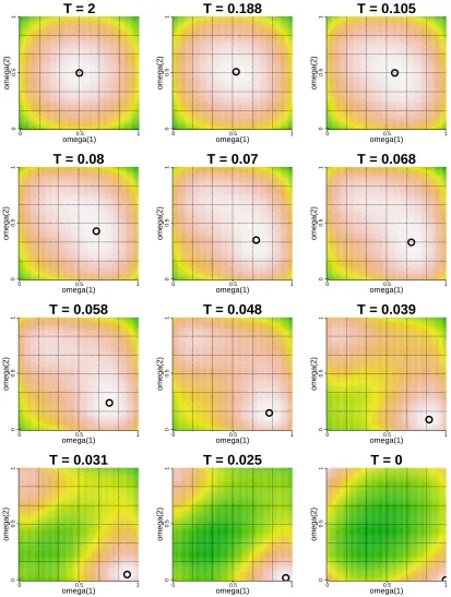
6.1 Visual Tracking of Annealing Process with a Toy Problem

The first experiment shows how the VMA2 method can solve the combinatorial optimization. Con-sider 3 variables and 1 factor, so that xi= (φ1·z1)λ1i+νi where all parameters exceptφ1are fixed

asΨ=I and∆=I. The likelihood function in (2) is then p(X|Z,Θ)∝exp(φ′_z

1Sφz1/2).Assume that

true edge on z31=1, indicating xi3←λi1, is known, but z11=1 and z21=0 are treated as unknown.

In what follows, we will show some simulation studies to provide insights and comparisons. The

data sets have n=100 data points drawn from the GFM with p=30 and ktrue=4,and withΨ=

0.05I and∆=diag(1.5,1.2,1.0,0.8). The zg j were independently generated with Pr(zg j =1) =

0.3, yielding roughly 70% sparsity; then, non-zero elements ofΦwhere generated as independent

standard normal variates, following whichΦZwas constrained to orthogonality.

To explore sensitivity to the chosen temperature schedule for annealing, experiments were run using three settings:

• (Log-inverse decay) Ti=3/log2(i+1)for i=1, . . . ,6999, and T7000=0

• (Linear decay) Ti=3−6×103×(i−1)for i=1, . . . ,1999, and T2000=0

• (Power decay) Ti=3×0.99−(i−1)for i=1, . . . ,1999, and T2000=0

For each, we evaluated the resulting MAP search in terms of comparison with the true model and

computational efficiency, in each case using a model with redundant factor dimension k=8.

6.3 Annealing with Fixed Hyper-parameters

(15)

0.0 0.2 0.4 0.6 0.8 1.0

0.0

0.2

0.4

0.6

0.8

1.0

False Positive Rate

True Positive Rate

0.0 0.2 0.4 0.6 0.8 1.0

0.0

0.2

0.4

0.6

0.8

1.0

False Positive Rate

True Positive Rate

Linear decay Log−inverse decay Exponential decay

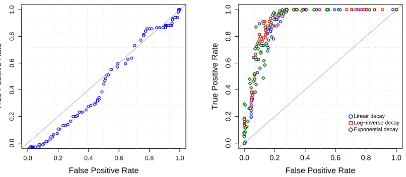
Figure 3: ROC for threshold PCA assuming a known, true k=4 factors (left), compared to VMA2

estimation of the GFM under the three cooling schedules and with k=8 (right). TPR

(vertical) and FPR (horizontal) were calculated according to TP/P and FP/N where P

and N denote the numbers of non-zero and zero elements in true loadings, TP and FP are the numbers of true positives and false positives, respectively.

schedules. The true positive (TPR) and false positive rates (FPR) were computed based on the

correspondences between estimated and true values of the zg j.For comparison, we used standard

PCA, extracting the dominant 4 eigenvectors and setting entries below a threshold (in absolute value) to zero; sliding the threshold towards zero gives a range of truncated loadings vectors in the PCA that define the ROC curve for this approach. The resulting ROC curve, shown in the left panel, is very near to the 45◦line, comparing very poorly with the annealed GFM; for the latter, each ROC curve indicates rather accurate identification of the sparse structure and the curves differ in small ways only as a function of cooling schedule. The choice of cooling schedule can, however, have a more marked influence on results if initialized at temperatures that are too low.

6.4 Inference on Degrees of Sparseness

A second analysis uses the sparsity prior p(ζg j) =

N

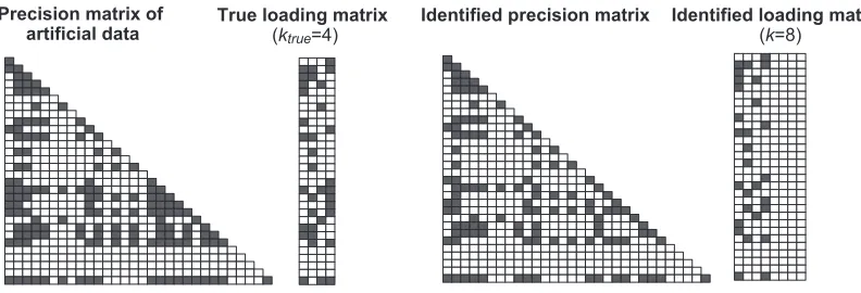
+(ζg j|µ,σ)with µ=3 andσ=6, and adopts the log-inverse cooling schedule. As shown in the right panel of Figure 4, the analysis realized

a reasonable control of FNR (15.4%) and FPR (0%), inducing a slightly less sparse solution than

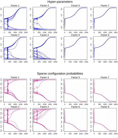
the true structure. The GFM analysis automatically prunes the redundant factors, identifying the true model dimension. Figure 5 displays a snapshot of evolving configuration probabilitiesωg jand

hyper-parametersζg j during the annealing schedule, demonstrating convergence over 2000 steps.

At around Ti≃0.45, all the configuration probabilities corresponding to the redundant four factors reached to zero.

(16)

Identified precision matrix Identified loading matrix

(k₌₈₎

Precision matrix of artificial data

True loading matrix

(k_true=4)

Figure 4: Result of the VMA2 estimation using the log-inverse rate cooling in analysis of synthetic data. (Left) Precision and factor loadings matrix used for generating the synthetic data

(p=30, ktrue=4). Non-zero elements are colored black. (Right) Estimated precision

and factor loadings matrix (k=8); note that the MAP estimate sets the last four loading vectors to zero and so identifies the true number of factors automatically.

• (Log-inverse decay) Ti=0.7/log2(i+1)for i=1, . . . ,6999 and,T7000=0

• (Linear decay) Ti=0.7−6×103×(i−1)for i=1, . . . ,1999 and,T2000=0

• (Power decay) Ti=0.7×0.99−(i−1)for i=1, . . . ,1999 and,T2000=0

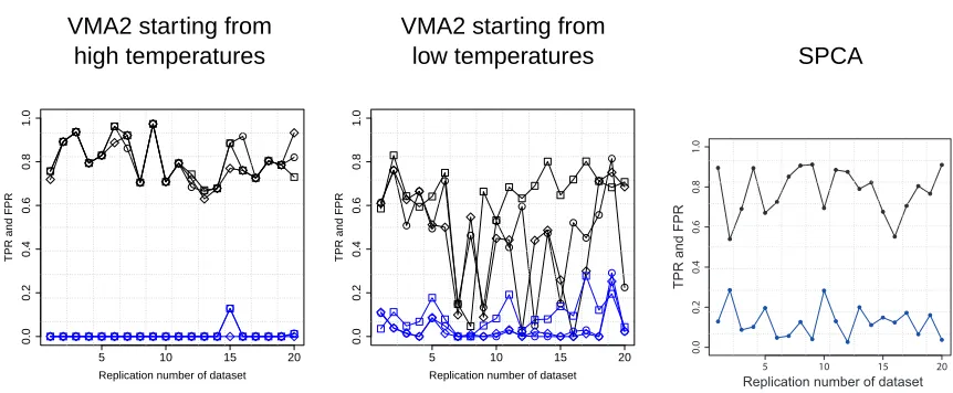
The initial temperatures are reduced from 3 to 0.7. Figure 6 shows the variations of TPR and FPR in the use of the six cooling schedules, evaluated in 20 analyses with replicated synthetic models and data sets. The left and center panels indicate significant dominance of the annealing starting from the higher initial temperatures. Performance in identifying model structure seriously degrades when using a temperature schedule that starts too low, and the sensitivity to schedule is very limited when beginning with reasonably high initial temperatures.

The right panel in Figure 6 shows TPR and FPR for the sparse PCA (SPCA) proposed by

Zou et al. (2006), evaluated on the same 20 data sets using theRcodespca()available at CRAN

(http://cran.r-project.org/). Withspca(), we can specify the number of nonzero elements

(cardinality) in each column of the factor loading matrix. We executedspca()after the assignment

of the true cardinality as well as the known factor dimension ktrue=4. The figure indicates a

better performance of GFM annealed with high initial temperature than the sparse PCA, and this

is particularly notable in that the GFM analysis uses k=8 and involves no a priori knowledge on

the degree of sparseness. It is important to see that the conducted comparison is biased since the data were drawn from the GFM with the orthogonal loading matrix where SPCA does not make orthogonality assumptions. In Section 7.1, we provide deeper comparisons among several existing sparse factor analyses based on image processing in hand-written digits recognition.

6.5 Computing Time Questions

(17)

Hyper-parameters

0 500 1000 1500 2000

0.0

1.0

2.0

3.0

Factor 1

0 500 1000 1500 2000

0.0

1.0

2.0

3.0

Factor 2

0 500 1000 1500 2000

0.0

1.0

2.0

3.0

Factor 3

0 500 1000 1500 2000

0.0

1.0

2.0

3.0

Factor 4

0 500 1000 1500 2000

0.0

1.0

2.0

3.0

Factor 5

0 500 1000 1500 2000

0.0

1.0

2.0

3.0

Factor 6

0 500 1000 1500 2000

0.0

1.0

2.0

3.0

Factor 7

0 500 1000 1500 2000

0.0

1.0

2.0

3.0

Factor 8

Sparse configuration probabilities

0 500 1000 1500 2000

0.0 0.2 0.4 0.6 0.8 1.0 Factor 1

0 500 1000 1500 2000

0.0 0.2 0.4 0.6 0.8 1.0 Factor 2

0 500 1000 1500 2000

0.0 0.2 0.4 0.6 0.8 1.0 Factor 3

0 500 1000 1500 2000

0.0 0.2 0.4 0.6 0.8 1.0 Factor 4

0 500 1000 1500 2000

0.0 0.2 0.4 0.6 0.8 1.0 Factor 5

0 500 1000 1500 2000

0.0 0.2 0.4 0.6 0.8 1.0 Factor 6

0 500 1000 1500 2000

0.0 0.2 0.4 0.6 0.8 1.0 Factor 7

0 500 1000 1500 2000

0.0 0.2 0.4 0.6 0.8 1.0 Factor 8

Figure 5: Convergence trajectories of theζg j (upper) andωg j (lower) in analysis of synthetic data over 2000 steps of annealed MAP estimation.

(18)

VMA2 starting from VMA2 starting from

high temperatures low temperatures SPCA

5 10 15 20

0.0

0.2

0.4

0.6

0.8

1.0

Replication number of dataset

TPR and FPR

5 10 15 20

0.0

0.2

0.4

0.6

0.8

1.0

TPR and FPR

5 10 15 20

0.0

0.2

0.4

0.6

0.8

1.0

TPR and FPR

Figure 6: Performance tests on 20 synthetic data sets for different cooling schedules and compari-son between the GFM and a sparse PCA (SPCA). For each panel, TPR (black) and FPR (blue) are plotted (vertical axis) against the 20 replicate simulations of artificial data. The results of annealing with the higher and lower initial temperatures are shown in the left and center panels respectively where the rates of cooling with log-inverse, linear and power decays are denoted by box, diamond and circle, respectively. The right panel shows the results of SPCA.

7. Real Data Applications

Experimental results on image analyses of hand-written digits (Section 7.1) and breast cancer gene expression data (Section 7.2) are shown to demonstrate practical relevance of the GFMs in analyses of high dimensional data.

7.1 Application: Hand-written Digit Recognition

We evaluate GFM in pattern recognition analyses of hand-written digit images, and make compar-isons to three existing methods; (i) SPCA (Zou et al., 2006), (ii) sparse probabilistic PCA with ARD prior (Archambeau and Bach, 2009), and (iii) MCMC-driven sparse factor analysis (West, 2003; Carvalho et al., 2008). These three methods are all based on models with non-orthogonal

sparse loading matrices. The training data set was made from 16×16 gray-scale images of 100

dig-its (i.e., n=100, p=256) of ‘3’ that were randomly drawn from the postal zip code data available

athttp://www-stat.stanford.edu/˜tibs/ElemStatLearn/(Hastie et al., 2001). To evaluate

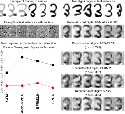
robustness of the four approaches, we added artificial outliers to 15 pixels (features) for about 5% of the original 100 images. Some of the contaminated images are shown in the top-left panels of Figure 8.

(19)

200 400 600 800 1000

0

200

400

600

800

1000

1200

Dimension of data

CPU time (sec)

Sparsity of True Loadings

Feature variables Factors 1234

200 400 600 800 1000

Identified Sparsity

Feature variables

Factors

12345678

200 400 600 800 1000

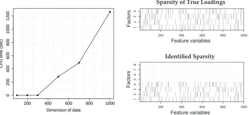
Figure 7: (Left) CPU times (in seconds; Intel(R) Core(TM)2 Duo processor, 2.60Ghz) versus model dimension p for the stochastic VMA2. For the deterministic VMA2, we terminated the

tests with the data larger than p=300. Execution times for the deterministic algorithm

were approximately 468, 812 and 1100 sec for p=100, 200 and 300. (Right) Identified

sparse loadings matrix, displayed as transpose, for the case of p=1000 where the MAP

estimation achieved FPR=12.0% and FNR=18.4%.

the methods, setting factor dimensions to k=10, we explored sparse estimates so that the degrees

of sparseness become approximately 30% (see Figure 8). For SPCA, we use the same number of non-zero elements in each loading vector as in the estimated GFM. The GFM was estimated using

VMA2 with a fixed value forζand a linear cooling schedule of length 2000.

A set of 100 test data samples was created from the 100 samples above by adding outliers

drawn from a uniform distribution to randomly-chosen pixels with probability 0.2. Performance

(20)

Example of training instances True digit images in test instances

Example of test instances with outliers Reconstructed digits: GFM (d.s.≈0.306)

Mean squared errors in data reconstruction Reconstructed digits: ARD-PPCA

Circle→Training error, Square→Test error (d.s.≈0.293)

GFM

ARD−PPCA

BFRM2.0

SPCA

0.10

0.20

0.30

0.40

0.50

0.60

Reconstructed digits: BFRM 2.0 (d.s.≈0.302)

Reconstructed digits: SPCA (d.s.≈0.306)

Figure 8: Comparison between GFM and the three alternative methods ((i)-(iii)) in the data

reconstruction of outlier hand-written digit images. For the implementation of

the sparse probabilistic PCA with ARD prior (ARD-PPCA), we prepared our own

R function which is available at Supplementary web site. In the application

of the MCMC-based sparse factor analysis, we used BFRM 2.0 distributed at http://www.stat.duke.edu/research/software/west/bfrm/. In the four panels on the bottom-right, d.s. denotes the degree of sparseness.

7.2 Application: Breast Cancer Gene Expression Study

(21)

20 60 100

50

200

xax Factor 1

20 60 100

50

200

xax Factor 2

20 60 100

20

60

xax Factor 3

20 60 100

10

40

70

Factor 4

20 60 100

10

30

50

xax Factor 5

20 60 100

2

6

10

xax Factor 6

20 60 100

10

30

xax Factor 7

20 60 100

5

15

Factor 8

20 60 100

5

15

xax Factor 9

20 60 100

0.5

1.5

2.5

xax Factor 10

20 60 100

2

6

10

xax Factor 11

20 60 100

5

15

Factor 12

20 60 100

5

15

xax Factor 13

20 60 100

2

6

10

xax Factor 14

20 60 100

2

8

14

xax Factor 15

20 60 100

1

3

5

7 Factor 16

20 60 100

1

3

5

xax Factor 17

20 60 100

2

8

14

xax Factor 18

20 60 100

5 15 xax Factor 19 200 400 600 800 1000

5 10 15 20 25

Genes

Factors

Identified Sparse Structure of Loading Matrix

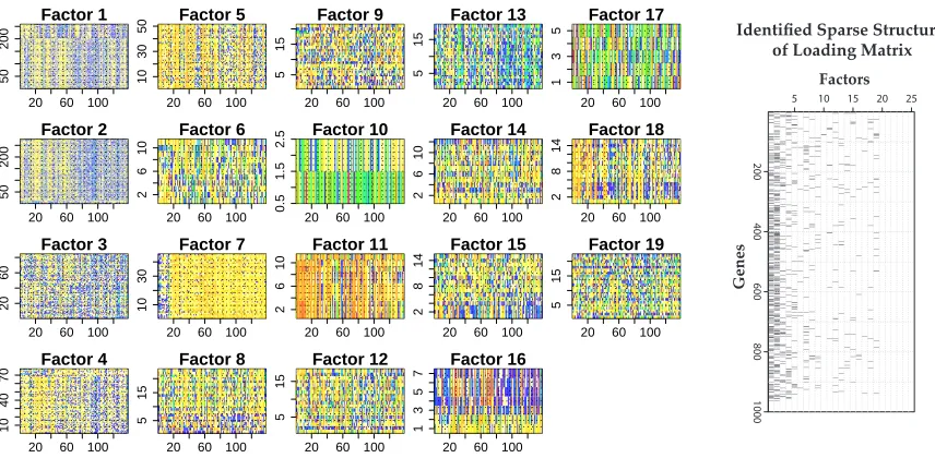
Figure 9: Identified factor probes (left) and sparse structure (right; binary matrix). In each image of the left panel, expression signatures of the probes associated with each factor are depicted across 138 samples (ordered along horizontal axis).

both statistical and biological aspects is available in supporting material at the first author’s web site (see link below).

Among the goals of most such studies are identification of multiple factors that may represent underlying activity of biological pathways and provide opportunities for improved predictive mod-els with estimated latent factors for physiological and clinical outcomes (e.g., Carvalho et al., 2008; Chang et al., 2009; Hirose et al., 2008; Lucas et al., 2006, 2009; West, 2003; Yoshida et al., 2004, 2006). Here we discuss an example application of our sparse GFM in analysis of data from previ-ously published breast cancer studies (Cheng et al., 2006; Huang et al., 2003; Pittman et al., 2004; West et al., 2001).

The GFM approach was applied to a sample of gene expression microarray data collected in the CODeX breast cancer genomics study (Carvalho et al., 2008; Pittman et al., 2004; West et al., 2001) at the Sun-Yat Sen Cancer Center, Taipei, during 2001-2004. In addition to summary expression indices from Affymetrix Human Genome U95 arrays, the data set includes immunohistochemistry (IHC) test for key hormonal receptor proteins in clinical prognostics; ERBB2 (Her2) and estrogen (ER). The IHC measures are discrete: ER negative (ER=0), ER positive with low/high-level expres-sion (ER=1 and ER=2), Her2 negative (Her2=0), and Her2 positive with low/high-level (Her2=1

and Her=2). We performed analysis of p=996 genes with the expression levels that, on a log2

(fold change) scale, exceed a median level of 7 and a range of at least 3-fold changes across the tumors. The data set, including the expression data and the IHC hormonal measures, are available on-line as supplementary material.

The annealed estimation of GFM was run with k=25, µ=7 andσ=10. The cooling schedule

(22)

pruning from the model maximum k=25. Heatmaps of gene expression for genes identified in each of the factors appear in Figure 9 with the identified sparse pattern of the loadings matrix.

Evaluation and Annotation of Inferred Factors: To investigate potential biological connections

of the factors, we evaluated enrichment of the functional annotations shared by genes in each factor through the Gene Ontology (GO). This exploration revealed associations between some factors and GO biological processes; the complete and detailed results, including tables of the GO enrichment analyses for each factor and detailed biological descriptions, are available from the web site of supporting information.

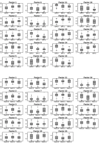
Factors Related to ER: Figure 10 displays boxplots of fitted values of the factor scores for

each sample, plotted across all 19 factors and stratified by levels of each of the clinical ER and Her2 (0/1/2) categories. For each sample i,the posterior mean of the factor vector, namely ˆλi= (Ik+∆)−1∆Φ′ZΨ−1/2xi,is evaluated at the estimated model, providing the fitted values displayed. We note strong association of ER status to factors 8 (GO: hormone metabolic process), 9 (GO: glucose metabolic process, negative regulation of MAPK activity), 12 (GO: C21-steroid hormone metabolic process), 14 (GO: apoptotic program, positive regulation of caspase activity), 18 (GO: M phase of meiotic cell cycle) and 19 (GO: regulation of Rab protein signal transduction). These clear relationships of ER status to multiple factors with intersecting but also distinct biological pathway annotations is consistent with the known complexity of the broader ER network, as estro-gen receptor-induced signaling impacts multiple cellular growth and developmentally related down-stream target genes and strongly defines expression factors linked to breast cancer progression.

Her2 Status and Oncogenomic Recombination Hotspot on 17q12: Figure 10 indicates factor 16

as strongly associated with Her2 status(0,1)versus 2. Factor 16 significantly loads on only 7 genes that include STARD3, GRB7 and two probe sets on the locus of ERBB2 (which encodes Her2). This is consistent with earlier gene expression studies that have consistently identified a single ex-pression pattern related to Her2 and a very small number of additional genes, and that have found the “low Her2 positives” level(1) to be generally comparable to negatives. Interestingly, we note that STARD3, GRB7 and ERBB2 are all located on the same chromosomal locus 17q12, which is known as PPP1R1B-STARD3-TCAP-PNMT-PERLD1-ERBB2-MGC14832-GRB7 locus. This locus has been reported in many studies (e.g., Katoh and Katoh, 2004) as an oncogenomic recombi-nation hotspot which is amplified frequently in breast tumor cells, and the purely exploratory (i.e., unsupervised) GFM analysis clearly identifies the “Her2 factor” as strongly reflective of increased expression of genes in this hotspot, consistent with the amplification inducing Her2 positivity.

Comparison to Non-sparse Analysis: Finally, we show a comparison to non-sparse traditional

(23)

ER:0 ER:1 ER:2

−30

0

20 Factor 1

ER:0 ER:1 ER:2

−20

0

20

Factor 2

ER:0 ER:1 ER:2

−10

5

15

Factor 3

ER:0 ER:1 ER:2

−20

−5

10

Factor 4

ER:0 ER:1 ER:2

−10

5

Factor 5

ER:0 ER:1 ER:2

−5

5

Factor 6

ER:0 ER:1 ER:2

−5

10

25

Factor 7

ER:0 ER:1 ER:2

−5

5

Factor 8

ER:0 ER:1 ER:2

−10

0

10

Factor 9

ER:0 ER:1 ER:2

−5

5

Factor 10

ER:0 ER:1 ER:2

−15

0

Factor 11

ER:0 ER:1 ER:2

−15

0

Factor 12

ER:0 ER:1 ER:2

−10

0

Factor 13

ER:0 ER:1 ER:2

−5

5

Factor 14

ER:0 ER:1 ER:2

−5

5

Factor 15

ER:0 ER:1 ER:2

−5

5

Factor 16

ER:0 ER:1 ER:2

−5

0

5

Factor 17

ER:0 ER:1 ER:2

−10

0

10

Factor 18

ER:0 ER:1 ER:2

−10

0

10 Factor 19

Her2:0 Her2:1 Her2:2

−30

0

Factor 1

−20

0

20

Factor 2

−10

5

15

Factor 3

−20

−5

10

Factor 4

−10

5

Factor 5

−5

5

Factor 6

−5

10

25

Factor 7

−5

5

Factor 8

−10

0

10

Factor 9

−5

5

Factor 10

−15

0

Factor 11

−15

0

Factor 12

−10

0

Factor 13

−5

5

Factor 14

−5

5

Factor 15

−5

5

Factor 16

−5

0

5

Factor 17

−10

0

10

Factor 18

−10

0

10 Factor 19

Figure 10: Boxplots of fitted values of breast tumor-specific factor scores, stratified by protein IHC determinations of clinical ER status (upper) and Her2 status (lower) in their 0/1/2 cate-gories.

8. Additional Comments

(24)

exhibiting the same patterns of covariances as the model/data predict, and the potential to induce robustness to outliers relative to non-graphical factor models, whether sparse or not. Some theoret-ical questions remain about precise conditions under which the sparsity patterns of covariance and precision matrices are guaranteed to agree in general sparse Gaussian factor models other than the GFM form. Additionally, extensions to integrate non-parametric Bayesian model components for factors, following Carvalho et al. (2008), are of clear future interest.

The ability of the VMA2 to aid in the identification of model structure in sparse GFM, and to provide an additional computational strategy and tools to address the inherently challenging com-binatorial optimization problem, has been demonstrated in our examples. Scaling to higher di-mensional models is enabled by relaxation of the direct deterministic optimization viewpoint, with stochastic search components that promote greater exploration of model space and can speed up search substantially. Nevertheless, moving to higher dimensions will require new, creative compu-tational implementations, such as using distributed computing, that will themselves require novel methodological concepts.

The annealed search methodology evidently will apply in other contexts beyond factor models. At one level, sparse factor models are an instance of problems of variable selection in multivari-ate regression, in which the regression predictors (feature variables) are themselves unknown (i.e., are the factors). The annealed entropy approach is therefore in principle applicable to problems involving regression model search and uncertainly in general classes of linear or nonlinear mul-tivariate regression with potentially many predictor variables. Beyond this, the same can be said about potential uses in other areas of graphical modelling involving structural inference of directed or undirected graphical models, and also in multivariate time series problems where some of the sparse structure may relate to relationships among variables over time.

We also remark on generalization of the basic form of VMA2 here that might use penalty func-tions other than the Shannon’s entropy used here. The central idea of the VMA2 is the design of a temperature-controlled iterative optimization that converges to the joint posterior distribution of model parameters and sparse structure indicators. The entropy formulation used in our GFM context was inspired by the form of the posterior itself, but similar algorithms—with the same con-vergent property—could be designed using other forms. This, along with computational efficiency questions and applications in models beyond the sparse GFM framework, and also potential ex-tensions to consider heavy-tailed or Bayesian nonparametric distributions for latent factors and/or residuals (e.g., Carvalho et al., 2008), are open areas for future research.

Acknowledgments

(25)

Appendix A.

We present a proof of Proposition 1 and a derivation of optimization overΦ.

A.1 Proof of Proposition 1

Replace the objective function of (5) by multiplying by inverse temperature 1/T :

1

T

G

T(Θ,ω) =_Z

∑

_∈_Zω(Z)log p(X,Z,Θ|ζ)

1/T₋

∑

Z∈Z

ω(Z)logω(Z).

An upper-bound of this modified criterion is derived as follows:

Z′_∈Z

p(Z′|X,Θ,ζ)1/T +K0

≤ K0.

In the second equality, the terms irrelevant to ω(Z) are included in K0 = log p(X,Θ|ζ)1/T+

log∑Z′_∈Z p(Z′|X,Θ,ζ)1/T. The first term in the second line is the negative of the Kullback-Leibler

divergence betweenω(Z)and the normalized tempered posterior distribution. The lower-bound of

the Kullback-Leibler divergence is attained if and only if

ω(Z) = p(Z|X,Θ,ζ)

1/T

∑Z′_∈Z p(Z′|X,Θ,ζ)1/T

,

as required.

A.2 Derivation: Optimization overΦ

Letρj, j∈ {1, . . . ,k}be the Lagrange multipliers to ensure the restrictions in (10). We now write down the Lagrange function:

φ′

jEω[S(zj,Ψ)]φj−ρj(kφjk2−1)−

∑

m6=j

ρmφ′mφj. (13)

Differentiation of (13) with respect toφ_jyields

E_ω_[_S₍_z_j_,Ψ_)]φ

j−ρjφj−

∑

m6=j

ρmφm=0. (14)

In order to solve this equation, the first step to be addressed is to find the closed form solution for the vector of the Lagrange multipliers,ρ₍₋_j₎={ρm}m=6 j∈Rk−1. Multiplying (14) by eachφ′m, m6= j, from the left, we have the k−1 equations as follows:

φ′

mEω[S(zj,Ψ)]φj−

∑

m6=j

(26)

This yields the matrix representation

Φ′

(−j)Eω[S(zj,Ψ)]φj−Φ′(−j)Φ(−j)ρ(−j)=0,

which in turn leads to the solution forρ₍₋_j₎as

ρ₍₋_j₎= (Φ′₍₋_j₎Φ₍₋_j₎)−1Φ′₍₋_j₎E_ω_[_S₍_z_j_,Ψ_)]φ

j.

Substituting this into the original Equation (14) yields the eigenvalue equation

NjEω[S(zj,Ψ)]φj−ρjφj=0 with Nj=I−Φ(−j)Φ′(−j). (15)

Now consider the alternative, symmetrized eigenvalue equation

NjEω[S(zj,Ψ)]Njϕj−ρjϕj=0. (16)

Since Nj is idempotent, left-multiplication of (16) by Njyields

NjEω[S(zj,Ψ)]Njϕj−ρjNjϕj=0.

which is equivalent to the required Equation (15) whenφ_j=Njϕj.

References

T.W. Anderson. An Introduction to Multivariate Statistical Analysis, 3rd ed. Wiley-Interscience; New Jersey, 2003.

C. Archambeau and F. Bach. Sparse probabilistic projections. In D. Koller, D. Schuurmans, Y. Ben-gio, and L. Bottou, editors, Advances in Neural Information Processing Systems 21, pages 73–80, Cambridge, MA, 2009. MIT Press.

H. Attias. Inferring parameters and structure of latent variable models by variational Bayes.

Pro-ceedings of the 15th Conference on Uncertainty in Artificial Intelligence (UAI99), pages 21–30,

1999.

C.M. Bishop. Probabilistic principal component analysis. Journal of the Royal Statistical Society

(Series B), 61:611–622, 1999.

C.M. Bishop. Pattern Recognition and Machine Learning, 1st ed. Springer: Singapore, 2006.

C.M. Carvalho and M. West. Dynamic matrix-variate graphical models. Bayesian Analysis, 2: 69–98, 2007.

C.M. Carvalho, J.E. Lucas, Q. Wang, J.T. Chang, J.R. Nevins, and M. West. High-dimensional sparse factor modelling: Applications in gene expression genomics. Journal of the American

Statistical Association, 103:1438–1456, 2008.