A Multiple Criteria Genetic Algorithm Scheduling Tool for Production
Scheduling in the Capital Goods Industry
Wenbin Xie
1, Chris Hicks
2, *, and Pupong Pongcharoen
31
Department of Electronics & Electrical Engineering, University of Strathclyde, Glasgow, Scotland.
2
Newcastle University Business School, Newcastle University, Newcastle upon Tyne, England.
3
Department of Industrial Engineering, Naresuan University, Phitsanulok, Thailand.
Received 15 June 2013; received in revised form 30 September 2013; accepted 26 October 2013
Abstract
Productionplannersusuallyaimtosatisfymultipleobjectives.Thispaperdescribesthedevelopmentofa
geneticalgorithmtoolthatfindsoptimumtrade-offsamongdeliveryperformance,resourceutilisation,and
work-in-progressinventory.Thetoolwasspecificallydevelopedtomeettherequirementsofcapitalgoodscompanies
that manufacture products with deep and complex product structures with components that have long and
complicatedroutings.Themodeltakesintoaccountoperationandassemblyprecedencerelationshipsandfinite
capacity constraints. The tool was tested using various production problems that were obtained from a
collaboratingcompany.Aseriesofexperimentsshowedthetoolprovidesasetofnon-dominatedsolutionsthat
enable the planner to choose an optimum trade-off according to their preferences. Previous research had
optimised a single objective function. This is the first scheduling tool of its type that has simultaneously
optimised delivery performance, resource utilisation and work-in-progress inventory. The quality of the
schedulesproducedwassignificantlybetterthantheapproachesusedbythecollaboratingcompany.
Keywords: genetic algorithms, capital goods, multiple criteria, production scheduling
1.
Introduction
Capital goods are “intended for use in production of other goods or services, rather than for final consumption” [1].
The capital goods industry is essential for economic success [2]. Production planning in capital goods companies is
particularly difficult because they produce highly customised, complex products in low volume on an engineer-to-order basis
[3]. Typical products such as power plant, ships and oilrigs have very complex product structures. These goods contain a
very diverse range of components. Some of these components are bespoke and are required in very low volume, whereas
some others are required in medium or large quantities. Certain components are highly customised whilst others are
standardised [3]. Price, life cycle cost and delivery performance are usually the most important order winning criteria [4].
Contracts often include severe penalties for lateness. Hicks [4] studied several capital goods companies and found that they
all had high levels of work-in-process inventory. The products were produced in very dynamic environments with many
uncertainties caused by supplier delays, machine breakdowns, rework, arrivals of new orders, etc. Rescheduling was
common and expected to complete in a relatively short time. Planners aim to optimise delivery performance, work in process
inventory and machine utilisation, but these factors are often conflicting. A practical and efficient scheduling tool, optimises
these criteria simultaneously, would provide a set of equally good solutions, each representing alternative trade-offs. The
decision maker could choose the solution that provides the best compromise taking into account of the market, finances, and
the status of the manufacturing system. This would help capital goods companies improve their competitiveness.
Theobjectivesofthispaperareto:
(1)
Provideabriefliteraturereviewtoidentifytheresearchgapaddressedbythiswork;
(2)
Describethedevelopmentoftheproposedalgorithm;
(3)
Applythenewtooltosolvethreeindustrialcasesobtainedfromacollaboratingcompany;
(4)
Comparetheperformanceofnewtoolwithprevioustools;
(5)
Presenttheconclusionsofthiswork.
2.
Literature Review
There is an abundant literature on production scheduling, but most research has focused on single machine, flow-shop
and job-shop scheduling [5]. The production scheduling of products with deep and complex product structure has been
largely neglected. Roman and Valle [6] studied dispatching rules and the effect of product structure on assembly shop
performance. Kim and Kim [7] used a genetic algorithm and simulated annealing for scheduling the production of products
with multiple levels of product structure. They used an aggregated model with only two resources; it was assumed that all
activities took place in either an assembly shop or a machine shop. This assumption was unrealistic because in practice
individual machining and assembly resources have different capabilities. Park and Kim [8] proposed a branch and bound
algorithm for an assembly system production scheduling problem. In their work, due dates were set as constraints rather than
as objectives, i.e. tardiness was not allowed. Pongcharoen et al. [9] developed a single objective genetic algorithm
scheduling tool (GAST) for scheduling products with deep product structure with multiple resource constraints. The tool
aimed to produce schedules that minimised a fitness function that combined holding and lateness costs. The limited research
has addressed scheduling approaches that are appropriate for capital goods companies. The application of multiple criteria
scheduling approaches in this context is currently a gap in the academic literature.
Multi-objective evolutionary algorithms (MOEAs) are meta-heuristics that adopt evolutionary principles to find the ‘fittest’ or set of ‘fittest’ offspring. These approaches are stochastic search methods. They cannot guarantee to find the best
solution but will able to find good solutions within a realistic time. These approaches are especially practical for
combinatorial optimisation problems with a large search spaces, which cannot be solved by enumerative search methods in
reasonable time [9]. One of the advantages of these approaches is that it is not necessary to have a detailed model of the
search space [10].
Genetic algorithms (GAs) have been particular popular and widely used for production scheduling optimisation
problems. GAs are particularly suitable for multiple criteria optimisation problems because they can simultaneously search
different regions of the search space and find a diverse set of solutions in discrete solution spaces [11]. The non-dominated
solutions form a Pareto set or Pareto Front [11, 12]. These solutions provide different compromises between the various
criteria. Qing-dao-er-ji et al. [13] proposed a hybrid genetic algorithm to solve job shop scheduling problems. This research
considered the simultaneous optimization of two criteria; make-span and inventory capacity. The hybrid GA used tailored
genetic operators and a local search operator which were designed to improve the local search capability. The effectiveness
of the approach was tested using a set of benchmark problems [14]. Lin et al. [15] developed two heuristics and a GA for
multiple objective scheduling problems on unrelated parallel machines. The three objectives considered were make-span,
total weighted completion time and total weighted tardiness. Each heuristics aimed to minimise a pair of these objectives
computationally efficient and provided reasonable quality solutions. The GA outperformed the two heuristics in terms of
both the number of non-dominated solutions and the quality of the solutions. Lei [16] conducted a survey of multiple
objective production scheduling and identified gaps in the field. He reported that most research had focused on typical
flow-shop scheduling problems (FSSP) and job-flow-shop scheduling problems (JSSP). There were no examples of research that had
considered delivery performance, work in process inventory and resource utilisation simultaneously. There were also no
examples of research that had addressed problems in hybrid systems, such as a combination of job-shop and assembly shops
of the type used in capital goods companies.
3.
Problem Description
Hicks [4] studies a range of capital goods companies and found that the price, product performance, life cycle, cost,
and delivery performance were the most important competitive criteria. Capital goods usually have deep and complex
product structures with many levels of assembly. Capital goods companies experience many uncertainties including the
arrival of new orders, engineering change, process times, machine breakdown, and rework. It was found that capital goods
companies had very high levels of work-in-process inventory. A major problem was that the supply of components and
subassemblies was often poorly coordinated with assembly processes. The high value of components was also another
important factor that led to high inventory levels. It is important that products are delivered on time, as contracts for the
supply of capital goods frequently including severe penalties for lateness. However, the early delivery of final product is
likely to be unacceptable to customers, because they need items to arrive for construction according to their project plan so
that the buildings and services are ready to receive the plant.
The products considered in this work have deep product structures. Hicks [4] proposed a hierarchical coding system
that provides full traceability for each item within the product structure. There may be multiple instances of like items at any
level of the product structure. The coding scheme includes product structure and product instance identifiers that can
uniquely identify and represent any item within the product structure [9]. Items at the root node represent a final product,
whilst the leaf nodes represent the components and other nodes in the hierarchy represent subassemblies. Many components
will have long routings and will require processing on many machines.
The proposed tool use a data model to operate and represents the real world manufacturing system. Input data may be
obtained from a manufacturing system simulation model developed by Hicks [3]. The model uses static and operational data.
The static data is the set of information that may not be changed during the scheduling process. This includes the product
structure and resources available. The operational data includes the schedule start time, the audit period, set-up, machining
and transfer times, planned due date, the customer due date, etc.
The model is deterministic and makes a number of assumptions:
(1) An operation cannot take place until the preceding operation is complete and an machine is available;
(2) A machine can only perform one operation at a time;
(3) There is no interruption of operations arising from machine breakdown;
(4) There is no rework;
(5) An assembly cannot start until the components are available.
4.
The Proposed Multiple Criteria GA Approach
Three objectives were considered simultaneously: i) delivery performance (DP); ii) work-in-process inventory (WIPI);
and iii) total idle time of machines (TITM). Production schedules were represented as a set of planned start and finish times
si start time of operation i;
ci completion time of operation i;
di due time of operation i;
ρ(i) the successor operation i;
r(i) the resource which performs operation i; σ(i) operation i on resource r(i);
φ(i) the operation that immediately succeeds the operation i on the resource r(i);
Ss start time of a planned production schedule;
Г the total operation set for production schedule; Τ the total resource set for production schedule;
ei unit time earliness costs for operation i (£500/day);
ti unit time tardiness costs for operation i (£1000/day);
i ei di ci i ti di ci
DP |( )| |( )| (1)
i ei c si
WIPI ( (i) ) (2)
)
( () () ()
) (
) (
i i i i
r s Ss s c
TITM (3)
4.1. Algorithm
The structure of the algorithm is shown in Fig. 1. It consists of: chromosome initialization, parameter setting;
population initialization, genetic operators; a repair process, fitness evaluation; selection schemes, and stopping criteria. The
details are explained in the following sections.
Fig. 1 Algorithm flow chart
4.2. Population initialisation
Production schedules were represented using the approach developed by Pongcharoen et al. [9] which represented
chromosomes as a sequence of operations on parts. The initial population was generated randomly using the Wichmann and
generating random numbers. This generator is computationally efficient and performs well with a very large period of
2.78×10¹³. It has been thoroughly tested and produces uniformly and independently distributed random numbers [18].
4.3. Genetic operations
The algorithm includes three alternative crossover operators: cycling crossover (CYX) [19]; position based crossover
(PBX) [20] and partially mapped crossover (PMX) [21]; and five alternative mutation operators: two operations adjacent
swap (2OAS) [22]; three operations adjacent swap (3OAS) [22]; scramble mutation (SM) [20]; inverse mutation (IM) [23];
and three operations random swap (3ORS) [22].
4.4. Repair process
The algorithm may produce infeasible schedules that contravene operation or assembly precedence relationships, or
exceed finite capacity constraints. Infeasible chromosomes are rectified using the four stage repair process proposed by
Pongcharoen et al. [24] and implemented and improved by Xie et al. [25]:
(1) Operation precedence adjustment;
(2) Part precedence adjustment;
(3) Deadlock adjustment;
(4) Timing assignment and capacity considerations.
4.5. Non-dominated ranking and fitness assignment
This is the first multiple criteria scheduling tool that simultaneously optimises delivery performance, resource
utilization, and work-in-progress inventory. The single objective approach proposed by Pongcharoen et al. [24] was
developed to include a new fitness measurement and assignment procedure to provide a mechanism for multiple criteria
optimisation. The methodology proposed by Fonseca and Fleming [26] was used. There are two major elements:
non-dominated ranking and niching. The ranking procedure ranks the population according to a dominance rule, and then each
solution is assigned a fitness value based on its rank rather than its fitness. Niching uses a fitness sharing strategy to
artificially decrease the fitness of solutions in densely populated area (σshare is the niche size or the radius of a niche). This
approach was based on the work of Deb [27]:
Step 1. Set counter i = 1 and specify the sharing parameter σshare. Initialise μ(j) = 0 (j = 1,…, N) for all ranks (the parameter
σshare represents the niche size, whilst μ(j) is the number of solutions within rank j).
Step 2. Compute the number of solutions (ni) that dominate solution i. Then compute and assign the rank (r) of solution i as
ri = 1 + ni. Increase the number of solutions in rank ri by one, so that μ(ri) = μ(ri) + 1;
Step 3. Repeat step 1 and step 2 until i < N (total number of solutions). Otherwise, go to step 4;
Step 4. Set a rank counter r = 1. Identify the maximum rank r* by checking the largest ri which has μ(ri) > 0. Assign
average fitness to solutions i = 1,...,N from the best rank 1 to worst rank n ≤ N using a linear function:
)
1
)
(
(
5
.
0
)
(
11 )
(
i
r
k avg
i
N
k
r
F
i
((4)
Step 5. Calculate the niche count for each solution i in rank ri with other solutions of the same rank by using Equation 5.
( ) 1(
)
i
r
j ij
i
sh
d
nc
(In Equation 5, dij is the normalised distance between any two solutions i and j in a rank and is calculated as follows:
M k k k j k i k ij f f f f d 1 2 min max ) ( ) ( ) ( ( (6)Where fkmax and fkmin are the maximum and minimum values of the kth objective. In equation 5, Equation 7 is used with
α = 1 to compute the sharing function value Sh(d) (α is a parameter that indicates whether the sharing effect between two
solutions reduces from one to zero linearly or non-linearly. When α=1, the effect reduces linearly).
; , 0 ; , ) ( 1 ) ( otherwise d if d d
sh ij share
share ij ij ( (7)
Step 6. After calculating the niche count, the shared fitness is calculated using the formula Fi(share) = Fi(avg) /nci. To preserve
the same average fitness, Fi(share) is multiplied by scaling factor S (shown in Equation 8) so that the scale fitness
value is the same as the original average fitness value.
( )1 ( ) )
(
.
(
)
/
i
r
k kshare
i avg
i
r
F
F
S
((8)
The scale fitness is:
) (share i scale S F
F (
(9)
Step 7. If r < r*, increment r by one and go to step 5. Otherwise, terminate the process.
4.6. Rank based roulette-elitist strategy (RRES)
The algorithm adopted the rank based roulette-elitist strategy to select which individuals survive to next generation.
This strategy, developed by Tunnukij et al. [28], combines the elite selection strategy [10] and the rank-based roulette wheel
[29]. It was found to be superior to other selection schemes for production scheduling in the capital goods industry [25]. The
strategy first selects 15% of the best chromosomes to survive to the next generation, it then uses the rank-based roulette
wheel to select the other 85% of chromosomes.
5.
Industrial Cases Study
Three industrial cases were studied in this research as shown in Table 1. These particular cases were chosen because
the size of these problems were large enough to allow the multiple objective scheduling tool to find a considerable number of
solutions but they were small enough to allow a large number of experiments to be conducted within a limited time period.
The experiments were based on a full factorial design [30].
Table 1 Characteristics of industrial cases
Case No. Product code No. of items Machining/assembly
operations = total No. of resources
Product structure levels
1 229 & 451 18 57/10 = 67 7 4
2 228 & 4 29 118/17 = 135 17 4
3 277 85 268/39 = 307 25 7
Pongcharoen et al. [24] developed a single criterion genetic algorithm scheduling tool (GAST) for production
tardiness of final products. Precedence relationships and finite capacity were considered. Fitness was evaluated by a single
objective function that combined earliness and tardiness costs. The results of the new multiple objective tool were compared
to the best schedules produced by the GAST to demonstrate the practicality and effectiveness of the tool. The configurations
considered are shown in Table 2. These configurations were chosen based on previous work by Xie et al. (2011) [31] and
Pongcharoen et al. (2001) [32].
Table 2 Experimental design
Configurations Case 1 Case 2 Case 3
Population size 100 100 200
No. of generations 40 40 80
Crossover operator PBX, PMX CYX, PMX CYX, PBX
Crossover probability 0.8 0.8 0.9
Mutation operator 3OAS, SM 3ORS, IM 2OAS, 3ORS
Mutation probability 0.01 0.01 0.01
Selection scheme RRES RRES RRES
σ (Niche size) 0.01, 0.03, 0.05, 0.1, 0.3, 0.5, 0.7, 0.9, 1.0
0.01, 0.03, 0.05, 0.1, 0.3, 0.5, 0.7, 0.9, 1.0
0.01, 0.03, 0.05, 0.1, 0.3, 0.5, 0.7, 0.9, 1.0
No. of replication 50 50 50
Total runs/case 1800 1800 1800
*Key: CYX: Cycling Crossover [33]; PBX: Position Base Crossover [20]; PMX: Partially Mapped Crossover [21]; 2OAS: Two
Operations Adjacent Swap [22]; 3OAS: Three Operations Adjacent Swap [22]; SM: Scramble Mutation [20]; IM: Inverse Mutation [10];
3ORS: Three Operations Random Swap [22]; RRES: Rank-based Roulette-Elitist Strategy [34]
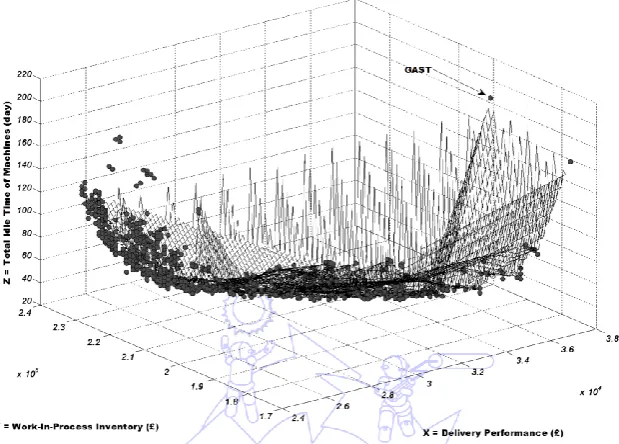
The Pareto optimal solutions obtained by the MOGAST are shown in figures 2, 3, and 4. The tool produced 1,108
different solutions for case 1, 1,545 solutions for case 2 and 452 for case 3. The delivery penalties for case 1 were within the
range of £1,900~£2,350 with work-in-process inventory within the range £4.5~£6.5x10⁴. The total idle time of machines was
within the range 10~50 days, the delivery penalty for case 2 was within the range £2.4~£3.8x10⁴ and the work-in-process
inventory was within the range £1.7~£2.4x10⁵. The total idle time for all machines was within the range 30~180 days, for
case 3, the delivery penalty was within the range £0~£4.5x10⁴ and the inventory costs were within the range £0~£3.0x10⁶,
whilst the total idle machine time was between 200~1,200 days.
Fig. 2 A 3D plot of the Pareto solutions (Case 1) 1900 1950 2000 2050 2100 2150 2200 2250 2300 2350 4.5 5 5.5 6 6.5
x 104 10 20 30 40 50 60 70 80 90 100
X = Delivery Performance (£ ) Y = Work-In-Process Inventory (£ )
The best schedule produced by the GAST [24] is displayed in the figure as a single dot that is highlighted by a pointed
arrow. It can be seen that the new tool produced far superior results to the GAST. For example, in case 3 the new tool
produced many schedules with near zero delivery penalties, with just a few hundred pounds of work-in-process inventory,
whilst the best schedule produced by GAST had a delivery penalty of £61,500 with £2.7m of work-in-process inventory; in
case 1, although GAST achieved a slightly better inventory cost than most of those from MCGAST, the results in terms of
delivery penalty and total idle time of machines were very inferior to those produced by the MCGAST. All the schedules
produced by the new tool had a higher machine utilisation rates than those generated by the GAST.
Fig. 3 A 3D plot of the Pareto optimal solutions (Case 2)
Fig. 4 A 3D plot of the Pareto optimal solutions (Case 3)
The computational time required by both tools is shown in Table 3. Both tools were run on the same UNIX time
sharing machine. It can be seen that the new tool is much faster than GAST. The speed of the tool is a very significant factor
if the tool is to be used by practitioners because rescheduling is very common and usually needs to be completed in a
relatively short period of time. The new tool is a few hundred times faster than GAST and will therefore be able to solve
Table 3 Computational time of both tools
CPU time (seconds)
Industrial data Gast MC Gast
Case 1 387 0.55~0.68
Case 2 1224 1.8~2.0
Case 3 3959 24~26
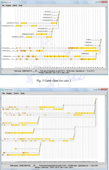
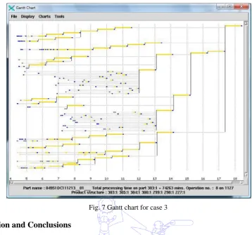
The tool proposed in this research contains a graphic user interface (GUI) that displays schedules as a Gantt chart.
With multiple objective scheduling problems, there is no best solution but a set of non-dominated solutions. The Gantt charts
for one of the solutions of each industrial case are shown in the following figures.
Fig. 5 Gantt chart for case 1
Fig. 7 Gantt chart for case 3
6.
Discussion and Conclusions
This research has developed a multiple criteria genetic algorithm scheduling tool that simultaneously minimises
work-in-process inventory and delivery penalties whilst maximising resource utilisation. The optimization of these criteria will
help capital goods companies compete in global markets. Previous work has only considered either one or two of these
factors. This is the first multiple criteria scheduling tool that has simultaneously considered these criteria for production
scheduling in the capital goods industry. The tool contains a repair process which is able to rectify all the infeasible
schedules due to product structure and machine capacity.
The new tool was able to produce a large number of schedules which found a large number of alternative optimum
trade-offs between the objectives. These schedules were all non-dominated solutions. The tool could improve the
competitiveness of companies. A decision maker could select from many equally good solutions based upon their experience,
current requirements, and preferences. The performance of the tool was compared with a previous single criterion tool that
used an objective function. The results demonstrated that the new tool achieved far better results for all the industrial cases
considered, especially for larger problems. The program produced results quickly, which would be helpful to planners. It
could be applied to solve much larger industrial cases which are very common in capital goods companies. The previous tool
(GAST) was limited to small industrial cases due to its slow speed. In practical scheduling situations, there are many
uncertainties. A fast scheduling tool is highly desirable so that planners can quickly reschedule work to achieve optimum
solutions.
References
[1] J. Black, N. Hashimzade, and G. Myles. A dictionary of economics 4th edition. Oxford: Oxford University Press, 2009. [2] N. Rosenberg, “Capital goods, technology and economic growth,” Oxford University Press, Oxford Economic Papers,
vol. 15, pp. 217-227, 2003.
[4] C. Hicks, “Computer aided production management (CAPM) systems in make-to-order / engineer-to-order heavy engineering companies,” Ph.D. dissertation, Faculty of Engineering, University of Newcastle, Newcastle upon Tyne, 1998.
[5] D. Lei, “Multi-objective production scheduling: A survey,” International Journal of Advanced Manufacturing Technology, vol. 43, pp. 925-938, 2009.
[6] D. B. Roman and A. G. del Vallei, “Dynamic assignation of due-dates in an assembly shop based in simulation,” International Journal of Production Research, vol. 34, pp. 1539-1554, June 1, 1996.
[7] J. U. Kim and Y. D. Kim, “Simulated annealing and genetic algorithms for scheduling products with multi-level product structure,” Computers Operations Research, vol. 23, pp. 857-868, 1996.
[8] M. W. Park and Y. D. Kim, “A branch and bound algorithm for a production scheduling problem in an assembly system under due date constraints,” European Journal of Operational Research, vol. 123, pp. 504-518, 2000.
[9] P. Pongcharoen, C. Hicks, P. M. Braiden, and D. J. Stewardson, “Determining optimum genetic algorithm parameters for scheduling the manufacturing and assembly of complex products,” International Journal of Production Economics, vol. 78, pp. 311-322, 2002.
[10] D. E. Goldberg, Genetic algorithms in search, optimisation and machine learning. Reading, MA: Addison-Wesley, 1989.
[11] A. Konak, D. W. Coit, and A. E. Smith, “Multi-objective optimization using genetic algorithms: A tutorial,” Reliability Engineering & System Safety, vol. 91, pp. 992-1007, 2006.
[12] C. A. C. Coello, “An updated survey of GA-based multiobjective optimization techniques,” ACM Computing Surveys, vol. 32, pp. 109-143, 2000.
[13] R. Qing-dao-er-ji, Y. Wang, and X. Wang, “Inventory based two-objective job shop scheduling model and its hybrid genetic algorithm,” Applied Soft Computing, vol. 13, pp. 1400-1406, Mar. 2013.
[14] S. R. Lawrence, “Resource constrained project scheduling: an experimental investigation of heuristic scheduling techniques,” Carnegie Mellon University, Pittsburgh1984.
[15] Y. K. Lin, J. W. Fowler, and M. E. Pfund, “Multiple-objective heuristics for scheduling unrelated parallel machines,” European Journal of Operational Research, vol. 227, pp. 239-253, June, 2013.
[16] D. Lei, “Multi-objective production scheduling: A survey,” International Journal of Advanced Manufacturing Technology, vol. 43, pp. 926-938, Aug. 2009.
[17] B. A. Wichmann and I. D. Hill, “An efficient and portable pseudo-random number generator,” Applied Statistics, vol. 31, pp. 188-190, 1982.
[18] F. A. Hossen, “Planning risk assessment in the manufacture of complex capital goods,” Ph.D. dissertation, School of Mechanical and Systems Engineering, University of Newcastle upon Tyne, 2006.
[19] I. M. Oliver, D. J. Smith, and J. R. C. Holland, “A study of permutation crossover operators on the traveling salesman problem,” Proceedings of the Second International Conference on Genetic Algorithms, Cambridge, Massachusette, USA, pp. 224-230, 1987.
[20] G. Syswerda, Scheduling optimisation using genetic algorithms. New York: Van Nostrand Reinhold, 1991.
[21] D. E. Goldberg and R. Lingle, “Alleles, loci and the travelling salesman problem,” in First International Conference on Genetic Algorithms and Their Applications, Hilladale, N.J., pp. 154-159, 1985.
[22] T. Murata and H. Ishibuchi, “Performance evaluation of genetic algorithms for flow shop scheduling problems,” Proceedings of the First IEEE International conference on Evolutionary Computation, Orlando, FL, pp. 812-817, 1994. [23] D. E. Goldberg, Genetic algorithms in search, optimization and machine learning. Reading, MA: Addison-wesley, 1989. [24] P. Pongcharoen, C. Hicks, and P. M. Braiden, “The development of genetic algorithms for the finite capacity
scheduling of complex products, with multiple levels of product structure,” European Journal of Operational Research, vol. 152, pp. 215-225, 2004.
[25] W. Xie, C. Hicks, and P. Pongcharoen, “An enhanced single-objective genetic algorithm scheduling tool for solving very large scheduling problems in capital goods industry,” in 16th International Working Seminar on Production Economics, Innsbruck, Austria, pp. 151-169, 2010.
[26] C. M. Fonseca and P. J. Fleming, “Genetic algorithms for multiobjective optimization: formulation, discussion and generalization,” Proceedings of the Fifth International Conference on Genetic Algorithms, Illinois, pp. 416-423, 1993. [27] K. Deb, Multi-objective optimization using evolutionary algorithms. Chichester: John Wiley & Sons, LTD, 2004. [28] T. Tunnukij and C. Hicks, “An enhanced grouping genetic algorithm for solving the cell formation problem,”
[29] C. R. Reeves, “Genetic algorithm for flowshop sequencing,” Computers and Operations Research, vol. 22, pp. 5-13, 1995.
[30] D. C. Montgomery, Design and analysis of experiments, 8th ed. New York: John Wiley & Sons, 2012.
[31] W. Xie, “Metaheuristics for single and multiple objectives production scheduling for the capital goods industry,” Ph.D. dissertation, Newcastle University Business School, Newcastle University, 2011.
[32] P. Pongcharoen, D. J. Stewardson, C. Hicks, and P. M. Braiden, “Applying designed experiments to optimize the performance of genetic algorithms used for scheduling complex products in the capital goods industry,” Journal of Applied Statistics, vol. 28, pp. 441-455, 2001.
[33] I. M. Oliver, C. J. Smith, and J. R. C. Holland, “A study of permutation crossover on the travelling salesmen problem, ” Proceeding of the Second International Conference on Genetic Algorithms and Their Applications, pp. 225-230, 1987. [34] T. Tunnukij, “An enhanced grouping genetic algorithm for optimising the formation of design teams and manufacturing