Posterior Regularization for Structured Latent Variable Models
Kuzman Ganchev [email protected]
Department of Computer and Information Science University of Pennsylvania
Levine 302, 3330 Walnut St Philadelphia PA, 19104, USA
João Graça [email protected]
L2F Inesc-ID Spoken Language Systems Lab R. Alves Redol, 9
1000-029 Lisboa, Portugal
Jennifer Gillenwater [email protected]
Ben Taskar [email protected]
Department of Computer and Information Science University of Pennsylvania
Levine 302, 3330 Walnut St Philadelphia PA, 19104, USA
Editor: Michael Collins
Abstract
We present posterior regularization, a probabilistic framework for structured, weakly supervised learning. Our framework efficiently incorporates indirect supervision via constraints on posterior distributions of probabilistic models with latent variables. Posterior regularization separates model complexity from the complexity of structural constraints it is desired to satisfy. By directly impos-ing decomposable regularization on the posterior moments of latent variables durimpos-ing learnimpos-ing, we retain the computational efficiency of the unconstrained model while ensuring desired constraints hold in expectation. We present an efficient algorithm for learning with posterior regularization and illustrate its versatility on a diverse set of structural constraints such as bijectivity, symmetry and group sparsity in several large scale experiments, including multi-view learning, cross-lingual de-pendency grammar induction, unsupervised part-of-speech induction, and bitext word alignment.1
Keywords: posterior regularization framework, unsupervised learning, latent variables models, prior knowledge, natural language processing
1. Introduction
In unsupervised problems where data has sequential, recursive, spatial, relational, and other kinds of structure, we often employ structured statistical models with latent variables to tease apart the underlying dependencies and induce meaningful semantic categories. Unsupervised part-of-speech and grammar induction, and word and phrase alignment for statistical machine translation in nat-ural language processing are examples of such aims. Generative models (probabilistic grammars,
graphical models, etc.) are usually estimated by maximizing the likelihood of the observed data by marginalizing over the hidden variables, typically via the Expectation Maximization (EM) al-gorithm. Because of computational and statistical concerns, generative models used in practice are very simplistic models of the underlying phenomena; for example, the syntactic structure of lan-guage or the lanlan-guage translation process. A pernicious problem with such models is that marginal likelihood may not guide the model towards the intended role for the latent variables, instead fo-cusing on explaining irrelevant but common correlations in the data. Since we are mostly interested in the distribution of the latent variables in the hope that they capture intended regularities without direct supervision, controlling this latent distribution is critical. Less direct methods such as clever initialization, ad hoc procedural modifications, and complex data transformations are often used to affect the posteriors of latent variables in a desired manner.
A key challenge for structured, weakly supervised learning is developing a flexible, declarative framework for expressing structural constraints on latent variables arising from prior knowledge and indirect supervision. Structured models have the ability to capture a very rich array of possible relationships, but adding complexity to the model often leads to intractable inference. In this article, we present the posterior regularization (PR) framework (Graça et al., 2007), which separates model complexity from the complexity of structural constraints it is desired to satisfy. Unlike parametric regularization in a Bayesian framework, our approach incorporates data-dependent constraints that are easy to encode as information about model posteriors on the observed data, but may be difficult to encode as information about model parameters through Bayesian priors. In Sections 5-8 we describe a variety of such useful prior knowledge constraints in several application domains.
The contributions of this paper are:
• A flexible, declarative framework for structured, weakly supervised learning via posterior regularization.
• An efficient algorithm for model estimation with posterior regularization.
• An extensive evaluation of different types of constraints in several domains: multi-view learn-ing, cross-lingual dependency grammar induction, unsupervised part-of-speech induction, and bitext word alignment.
• A detailed explanation of the connections between several other recent proposals for weak supervision, including structured constraint-driven learning (Chang et al., 2007), generalized expectation criteria (Mann and McCallum, 2008, 2007) and Bayesian measurements (Liang et al., 2009).
The rest of this paper is organized as follows. Section 2 describes the posterior regularization framework and Section 3 illustrates the range of different types of weak supervision constraints representable in our framework. Section 4 describes the relationship between posterior regulariza-tion and other related frameworks. Secregulariza-tions 5-8 describe applicaregulariza-tions of PR to several problems: word alignment (§5), multi-view learning (§6), cross-lingual projection (§7) and inducing sparsity structure (§8). Section 9 concludes the paper and presents areas for future work.
2. Posterior Regularization Framework
show, this allows tractable learning and inference even when the constraints would be intractable to encode directly in the model parameters. By defining a flexible language for specifying diverse types of problem-specific prior knowledge, we make the framework applicable to a wide variety of probabilistic models, both generative and discriminative. In Sections 2.1-2.7 we will focus on generative models, and describe the case of discriminative models in Section 2.8. We will use a problem from natural language processing as a running example in the exposition:
Running Example The task is part-of-speech (POS) tagging with limited or no training data.
Suppose we know that each sentence should have at least one verb and at least one noun, and would like our model to capture this constraint on the unlabeled sentences. The model we will be using is a first-order hidden Markov model (HMM).
We describe four other applications with empirical results in Sections 5-8, but it will be easier to illustrate key concepts using this simple example.
2.1 Preliminaries and Notation
We assume that there is a natural division of variables into “input” variables x and “target” variables y for each data instance, where x’s are always observed. We denote the set of all instances of unlabeled data as X. In case of semi-supervised learning, we have some labeled data as well, and we will use the notation(XL,YL)to denote all the labeled instances.
The starting point for using the PR framework is a probabilistic model. Letθbe the parameters of the model. For now we assume a generative model pθ(x,y), and we use
L
(θ) =log pθ(XL,YL) + log∑Ypθ(X,Y) +log p(θ)to denote the parameter-regularized log-likelihood of the data.Running Example In the POS tagging example from above, we would use x={x1,x2, . . .x|x|}
to denote a sentence (i.e., a sequence of words xi) and y={y1,y2, . . .y|x|}to denote a possible
POS assignment. Using an HMM, it is defined in the normal way as:
pθ(x,y) = |x|
∏
i=1
pθ(yi|yi−1) pθ(xi|yi),
withθrepresenting the multinomial distributions directly, and where pθ(y1|y0) =pθ(y1)
rep-resents a set of initial probabilities. Suppose we have a small labeled corpus and a larger unlabeled corpus. For a generative model such as an HMM, the log-likelihood (+ log-prior) is:
L
(θ) =log pθ(XL,YL) +log∑
Y
pθ(X,Y) +log p(θ),
where corpus probabilities are products over instances: pθ(x,y) =∏pθ(x,y) and analo-gously for XL,YL; and where p(θ)is a prior distribution over the parametersθ.
2.2 Regularization via Posterior Constraints
specified with sets
Q
of allowed distributions over the hidden variables y. We will defineQ
in terms of constraint featuresφ(X,Y)and their expectations.2Running Example Recall that in our running example, we want to bias learning so that each
sentence is labeled to contain at least one verb. To encode this formally, we define a feature φ(x,y) =“number of verbs in y”, and require that this feature has expectation at least 1. For consistency with the rest of the exposition and standard optimization literature, we will use the equivalentφ(x,y) =“negative number of verbs in y” and require this has expectation at most -1:3
Q
x={qx(y) : Eq[φ(x,y)]≤ −1}.Note that we enforce the constraint only in expectation, so there might be a labeling with non-zero probability that does not contain a verb. To actually enforce this constraint in the model would break the first-order Markov property of the distribution.4 In order to also require at least one noun per sentence in expectation, we would add another constraint feature, so that φwould be a function from x,y pairs toR2.
We define
Q
, the set of valid distributions, with respect to the expectations of constraint features, rather than their probabilities, so that our objective leads to an efficient algorithm. As we will see later in this section, we also require that the constraint features decompose as a sum in order to ensure an efficient algorithm. More generally than in the running example, we will define constraints over an entire corpus:Constrained Posterior Set :
Q
={q(Y): Eq[φ(X,Y)]≤b}.In words,
Q
denotes the region where constraint feature expectations are bounded by b. Addi-tionally, it is often useful to allow small violations whose norm is bounded byε≥0:Constrained Set(with slack):
Q
={q(Y):∃ξ,Eq[φ(X,Y)]−b≤ξ;||ξ||β≤ε}. (1) Hereξ is a vector of slack variables and||·||β denotes some norm. Note that the PR method we describe will only be useful ifQ
is non-empty:Assumption 2.1
Q
is non-empty.We explore several types of constraints in Sections 5-8, including: constraints similar to the running example, where each hidden state is constrained to appear at most once in expectation; constraints that bias two models to agree on latent variables in expectation; constraints that en-force a particular group-sparsity of the posterior moments. The constraint set defined in Equation 1 is usually referred to as inequality constraints with slack, since setting ε=0 enforces inequality constraints strictly. The derivations for equality constraints are very similar to the derivations for inequality so we leave them out in the interest of space. Note also that we can encode equality
2. Note: the constraint features do not appear anywhere in the model. If the model has a log-linear form, then it would be defined with respect to a different set of model features, not related to the constraint features we consider here. 3. Note that the distribution qxandQxdepend on x because the featuresφ(x,y)might depend on the particular example
x.
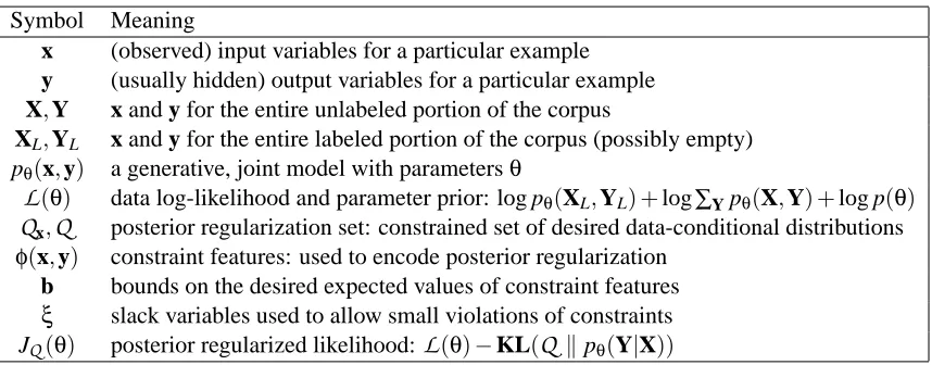
Symbol Meaning
x (observed) input variables for a particular example y (usually hidden) output variables for a particular example X,Y x and y for the entire unlabeled portion of the corpus
XL,YL x and y for the entire labeled portion of the corpus (possibly empty)
pθ(x,y) a generative, joint model with parametersθ
L
(θ) data log-likelihood and parameter prior: log pθ(XL,YL) +log∑Ypθ(X,Y) +log p(θ)Q
x,Q
posterior regularization set: constrained set of desired data-conditional distributionsφ(x,y) constraint features: used to encode posterior regularization b bounds on the desired expected values of constraint features
ξ slack variables used to allow small violations of constraints
JQ(θ) posterior regularized likelihood:
L
(θ)−KL(Q
kpθ(Y|X))Table 1: Summary of notation used.
constraints by adding two inequality constraints, although this will leave us with twice as many variables in the dual. The assumption of linearity of the constraints is computationally important, as we will show below. For now, we do not make any assumptions about the featuresφ(x,y), but if they factor in the same way as the model, then we can use the same inference algorithms in PR training as we use for the original model (see Proposition 2.2). In PR, the log-likelihood of a model is penalized with the KL-divergence between the desired distribution space
Q
and the model posteriors,KL(
Q
k pθ(Y|X)) =minq∈QKL(q(Y)k pθ(Y|X)).
The posterior-regularized objective is:
Posterior Regularized Likelihood : JQ(θ) =
L
(θ)−KL(Q
kpθ(Y|X)). (2)Negative Log-Likelihood representable
by model
Q
p(Y)p(X)
pθ(X) δ(X)
KL(Q||p θ(Y|X
))
pθ(Y|X)
KL(δ
(X)||pθ(X ))
θ
Posterior Regularization q(Y)
Θ
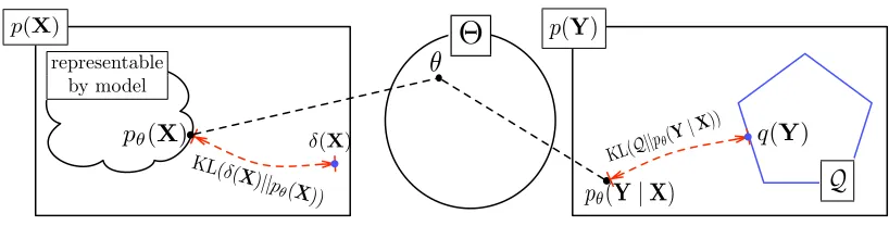
Figure 1: An illustration of the PR objective for generative models, as a sum of two KL terms. The symbolΘrepresents the set of possible model parameters,δ(X)is a distribution that puts probability 1 on X and 0 on all other assignments. Consequently KL(δ(X)||pθ(X)) =
L
(θ). (We ignore the parameter prior and additional labeled data in this figure for clarity.)the posterior distribution pθ(Y|X). PR adds to the maximum likelihood objective a corresponding KL distance for this distribution. If
Q
has only one distribution, then we recover labeled maximum likelihood training. This is one of the justifications for the use and the particular direction of the KL distance in the penalty term.Running Example In order to represent a corpus-wide constraint set
Q
for our POS prob-lem, we stack the constraint features into a function from X,Y pairs (sentences, part-of-speechsequences) toR2|X|, where|X|is the number of sentences in our unlabeled corpus. For the POS tagging example, the PR objective penalizes parameters that do not assign each sentence at least one verb and one noun in expectation.
For PR to be successful, the model pθ(Y|X) has to be expressive enough to ensure that the learned model has posteriors pθ(Y|X)in or nearly in
Q
. Even if that is the case, the same parameters might not ensure that the constraints are satisfied on a test corpus, so we could also use q(Y) = arg minq′∈QKL(q′(Y)k pθ(Y|X)) for prediction instead of pθ(Y|X). We will see in Sections 5and 7 that this sometimes results in improved performance. Chang et al. (2007) report similar results for their constraint-driven learning framework.
2.3 Slack Constraints vs. Penalty
In order for our objective to be well defined,
Q
must be non-empty. When there are a large number of constraints, or when the constraint features φare defined by some instance-specific process, it might not be easy to choose constraint values b and slackε that lead to satisfiable constraints. It is sometimes easier to penalize slack variables instead of setting a boundεon their norm. In these cases, we add a slack penalty to the regularized likelihood objective in Equation 2:L
(θ) − minq,ξ KL(q(Y)||pθ(Y|X)) +σ||ξ||β
s.t. Eq[φ(X,Y)]−b≤ξ.
The slack-constrained and slack-penalized versions of the objectives are equivalent in the sense that they follow the same regularization path: for everyεthere exists someσthat results in identical parameters θ. Note that while we have used a norm ||·||β to impose a cost on violations of the constraints, we could have used any arbitrary convex penalty function, for which the minimal q is easily computable.
2.4 Computing the Posterior Regularizer
In this subsection, we describe how to compute the objective we have introduced for fixed parame-tersθ. The regularization term is stated in Equations 2 and 3 in terms of an optimization problem. We assume that we have algorithms to do inference5 in the statistical model of interest, pθ. We describe the computation of the regularization term for the inequality constraints:
min
q,ξ KL(q(Y)kpθ(Y|X)) s.t. Eq[φ(X,Y)]−b≤ξ; ||ξ||β≤ε. (4)
Proposition 2.1 The regularization problems for PR with inequality constraints in Equation 4 can
be solved efficiently in its dual form. The primal solution q∗is unique since KL divergence is strictly convex and is given in terms of the dual solutionλ∗by:
q∗(Y) = pθ(Y|X)exp{−λ
∗·φ(X,Y)}
Z(λ∗) (5)
where Z(λ∗) =∑Ypθ(Y|X)exp{−λ∗·φ(X,Y)}. Define||·||β∗ as the dual norm of||·||β. The dual of the problem in Equation 4 is:
max
λ≥0 −b·λ−log Z(λ) −ε||λ||β∗. (6)
The proof is included in Appendix B using standard Lagrangian duality results and strict convex-ity of KL (e.g., Bertsekas, 1999). The dual form in Equation 6 is typically computationally more tractable than the primal form (Equation 4) because there is one dual variable per expectation con-straint, while there is one primal variable per labeling Y. For structured models, this is typically intractable. An analogous proposition can be proven for the objective with penalties (Equation 3), with almost identical proof. We omit this for brevity.
2.5 Factored q(Y)for Factored Constraints
The form of the optimal q with respect to pθ(Y|X)andφhas important computational implications. Proposition 2.2 If pθ(Y|X) factors as a product of clique potentials over a set of cliques
C
, and φ(X,Y)factors as a sum over some subset of those cliques, then the optimizer q∗(Y)of Equation 5 will also factor as a product of potentials of cliques inC
.This is easy to show. Our assumptions are a factorization for pθ: Factored Posteriors : p(Y|X) = 1
Z(X)c
∏
∈Cψ(X,Yc)M−Step: max
θ F(q, θ)
E′
−Step: max
q∈QF(q, θ)
θ
q(Y)
Q pθ(Y|X)
q(Y) min KL
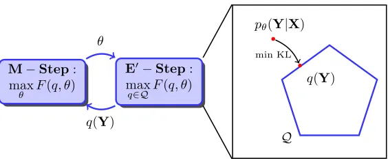
Figure 2: Modified EM for optimizing generative PR objective
L
(θ)−KL(Q
kpθ(Y|X)).and the same factorization forφ:
Factored Features : φ(X,Y) =
∑
c∈C
φ(X,Yc)
which imply that q∗(Y)will also factor as a product over the cliques
C
:Factored Solution : q∗(Y) = 1
Z(X)Z(λ)c
∏
∈Cψ(X,Yc) exp{−λ·φ(X,Yc)}= 1
Z′(X)c
∏
∈Cψ ′(X,Yc),
whereψ′(X,Yc) =ψ(X,Yc)exp{−λ·φ(X,Yc)}and Z′(X) =Z(X)Z(λ).
2.6 Generative Posterior Regularization via Expectation Maximization
This section presents an optimization algorithm for the PR objective. The algorithm we present is a minorization-maximization algorithm akin to EM, and both slack-constrained and slack-penalized formulations can be optimized using it. To simplify the exposition, we focus first on slack-constrained version, and leave a treatment of optimization of the slack-penalized version to Section 2.7.
Recall the standard expectation maximization (EM) algorithm used to optimize marginal likeli-hood
L
(θ) =log∑Ypθ(X,Y). Again, for clarity of exposition, we ignore log p(θ), the prior onθ, as well as log pθ(XL,YL), the labeled data term, as they are simple to incorporate, just as in regular EM. Neal and Hinton (1998) describe an interpretation of the EM algorithm as block coordinate ascent on a function that lower-boundsL
(θ), which we also use below. By Jensen’s inequality, we define a lower-bound F(q,θ)asL
(θ) =log∑
Y
q(Y)pθ(X,Y)
q(Y) ≥
∑
Y q(Y)logpθ(X,Y)
we can re-write F(q,θ)as
F(q,θ) =
∑
Y
q(Y)log(pθ(X)pθ(Y|X))−
∑
Y
q(Y)log q(Y)
=
L
(θ)−∑
Y
q(Y)log q(Y)
pθ(Y|X) =
L
(θ)−KL(q(Y)||pθ(Y|X)).Using this interpretation, we can view EM as performing coordinate ascent on F(q,θ). Starting from an initial parameter estimateθ0, the algorithm iterates two block-coordinate ascent steps until a convergence criterion is reached:
E : qt+1=arg max q
F(q,θt) =arg min q
KL(q(Y)k pθt(Y|X)),
M :θt+1=arg max θ F(q
t+1,θ) =arg max
θ Eqt+1[log pθ(X,Y)]. (7) It is easy to see that the E-step sets qt+1(Y) =pθt(Y|X).
The PR objective (Equation 2) is
JQ(θ) =max
q∈Q F(q,θ) =
L
(θ)−q(minY)∈QKL(q(Y)||pθ(Y|X)),where
Q
={q(Y):∃ξ, Eq[φ(X,Y)]−b≤ξ; ||ξ||β≤ε}. In order to optimize this objective, it suffices to modify the E-step to include the constraints:E′: qt+1=arg max q∈Q
F(q,θt) =arg min q∈Q
KL(q(Y)kpθt(Y|X)). (8)
The projected posteriors qt+1(Y) are then used to compute sufficient statistics and update the model’s parameters in the M-step, which remains unchanged, as in Equation 7. This scheme is illustrated in Figure 2.
Proposition 2.3 The modified EM algorithm illustrated in Figure 2, which iterates the modified
E-step (Equation 8) with the normal M-E-step (Equation 7), monotonically increases the PR objective: JQ(θt+1)≥JQ(θt).
Proof: The proof is analogous to the proof of monotonic increase of the standard EM objective. Essentially,
JQ(θt+1) =F(qt+2,θt+1)≥F(qt+1,θt+1)≥F(qt+1,θt) =JQ(θt).
The two inequalities are ensured by the E′-step and M-step. E′-step sets qt+1=arg maxq∈QF(q,θt), hence JQ(θt) =F(qt+1,θt). The M-step sets θt+1 =arg maxθF(qt+1,θ), hence F(qt+1,θt+1)≥
F(qt+1,θt). Finally, JQ(θt+1) =maxq∈QF(q,θt+1)≥F(qt+1,θt+1)
Note that the proposition is only meaningful when
Q
is non-empty and JQ is well-defined.As for standard EM, to prove that coordinate ascent on F(q,θ) converges to stationary points of
JQ(θ), we need to make additional assumptions on the regularity of the likelihood function and
boundedness of the parameter space as in Tseng (2004). This analysis can be easily extended to our setting, but is beyond the scope of the current paper.
Running Example For the POS tagging example with zero slack, the optimization problem
we need to solve is:
arg min q
KL(q(Y)kpθ(Y|X)) s.t. Eq[φ(X,Y)]≤ −1
where 1 is a vector of with 1 in each entry. The dual formulation is given by
arg max λ≥0
1·λ−log Z(λ) with q∗(Y) = pθ(Y|X)exp{−λ
∗·φ(X,Y)}
Z(λ∗) . (9)
We can solve the dual optimization problem by projected gradient ascent. The HMM model can be factored as products over sentences, and each sentence as a product of emission prob-abilities and transition probprob-abilities.
pθ(y|x) =∏ |x|
i=1pθ(yi|yi−1)pθ(xi|yi)
pθ(x) (10)
where pθ(y1|y0) = pθ(y1) are the initial probabilities of our HMM. The constraint features
φcan be represented as a sum over sentences and further as a sum over positions in the sentence:
φ(x,y) = |x|
∑
i=1
φi(x,yi) = |x|
∑
i=1
(−1,0)⊤ if yiis a verb in sentence x
(0,−1)⊤ if y
iis a noun in sentence x
(0,0)⊤ otherwise
(11)
combining the factored Equations 10 and 11 with the definition of q(Y)we see that q(Y)must also factor as a first-order Markov model for each sentence:
q∗(Y)∝
∏
x∈X
|x|
∏
i=1
pθ(yi|yi−1)pθ(xi|yi)e−λ ∗·φ
i(x,yi).
Hence q∗(Y)is just a first-order Markov model for each sentence, and we can compute the normalizer Z(λ∗)and marginals q(yi)for each example using forward-backward. This allows
computation of the dual objective in Equation 9 as well as its gradient efficiently. The gradient of the dual objective is 1−Eq[φ(X,Y)]. We can use projected gradient (Bertsekas, 1999) to
perform the optimization, and the projection can be done sentence-by-sentence allowing for online optimization such as stochastic gradient. Optimization for non-zero slack case can be done using projected subgradient (since the norm is not smooth).
Note that on unseen unlabeled data, the learned parametersθmight not satisfy the constraints on posteriors exactly, although typically they are fairly close if the model has enough capacity.
2.7 Penalized Slack via Expectation Maximization
If our objective is specified using slack-penalty such as in Equation 3, then we need a slightly different E-step. Instead of restricting q∈
Q
, the modified E′-step adds a cost for violating the constraintsE′: min
q,ξ KL(q(Y)||pθ(Y|X)) + σ||ξ||β
s.t. Eq[φ(X,Y)]−b≤ξ.
An analogous monotonic improvement of modified EM can be shown for the slack-penalized ob-jective. The dual of Equation 12 is
max
λ≥0 −b·λ−log Z(λ) s.t. ||λ||β∗≤σ. 2.8 PR for Discriminative Models
The PR framework can be used to guide learning in discriminative models as well as generative models. In the case of a discriminative model, we only have pθ(y|x), and the likelihood does not depend on unlabeled data. Specifically,
L
D(θ) =log pθ(YL|XL) +log p(θ),where(YL,XL)are any available labeled data and log p(θ)is a prior on the model parameters. With this definition of
L
(θ)for discriminative models we will optimize the discriminative PR objective (zero-slack case):Discriminative PR Likelihood : JQD(θ) =
L
D(θ)−KL(Q
kpθ(Y|X)). (13) In the absence of both labeled data and a prior on parameters p(θ), the objective in Equation 2 is optimized (equal to zero) for any pθ(Y|X)∈Q
. If we employ a parametric prior on θ, then we will prefer parameters that come close to satisfying the constraints, where proximity is measured by KL-divergence.Running Example For the POS tagging example, our discriminative model might be a first
order conditional random field. In this case we model:
pθ(y|x) =exp{θ·f(x,y)}
Zθ(x)
where Zθ(x) =∑yexp{θ·f(x,y)}is a normalization constant and f(x,y)are the model fea-tures. We will use the same constraint features as in the generative case:φ(x,y) =“negative number of verbs in y”, and define
Q
x and qx also as before. Note that f are features used to define the model and do not appear anywhere in the constraints whileφ are constraint features that do not appear anywhere in the model.Traditionally, the EM algorithm is used for learning generative models (the model can condition on a subset of observed variables, but it must define a distribution over some observed variables). The reason for this is that EM optimizes marginal log-likelihood (
L
in our notation) of the observed data X according to the model. In the case of a discriminative model, pθ(Y|X), we do not model the distribution of the observed data, the value ofL
Das a function ofθdepends only on the para-metric prior p(θ) and the labeled data. By contrast, the PR objective uses the KL term and the corresponding constraints to bias the model parameters. These constraints depend on the observed data X and if they are sufficiently rich and informative, they can be used to train a discriminative model. In the extreme case, consider a constraint setQ
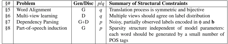
that contains only a single distribution q, with q(Y∗) =1. So, q is concentrated on a particular labeling Y∗. In this case, the PR objective in Equation 13 reduces to§# Problem Gen/Disc p/q Summary of Structural Constraints
§5 Word Alignment G q Translation process is symmetric and bijective §6 Multi-view learning D q Multiple views should agree on label distribution §7 Dependency Parsing G+D p Noisy, partially observed labels encoded inφand b §8 Part-of-speech induction G p Sparsity structure independent of model parameters:
each word should be generated by a small number of POS tags
Table 2: Summary of applications of Posterior Regularization described in this paper. Gen/Disc refers to generative or discriminative models. The p/q column shows whether we use the original model p or the projected distribution q at decode time.
Thus, if
Q
is informative enough to uniquely specify a labeling of the unlabeled data, the PR objec-tive reduces to the supervised likelihood objecobjec-tive. WhenQ
specifies a range of distributions, such as the one for multi view learning (Section 6), PR biases the discriminative model to have pθ(Y|X) close toQ
.Equation 13 can also be optimized with a block-coordinate ascent, leading to an EM style algo-rithm very similar to the one presented in Section 2.6. We define a lower bounding function:
F′(q,θ) =−KL(q(Y)kpθ(Y|X)) =
∑
Y
q(Y)logpθ(Y|X)
q(Y) .
Clearly, maxq∈QF′(q,θ) =−KL(
Q
kpθ(Y|X))so F′(q,θ)≤ −KL(Q
kpθ(Y|X))for q∈Q
.The modified E′and M′ steps are:6 E′: qt+1=arg max
q∈Q
F′(q,θt) =arg min q∈Q
KL(q(Y)kpθt(Y|X)),
M′:θt+1=arg max
θ F
′(qt+1,θ) =arg max θ Eq
t+1[log pθ(Y|X)]. (14)
Here the difference between Equation 7 and Equation 14 is that now there is no generative compo-nent in the lower-bound F′(q,θ)and hence we have a discriminative update to the model parameters in Equation 14.
3. Summary of Applications
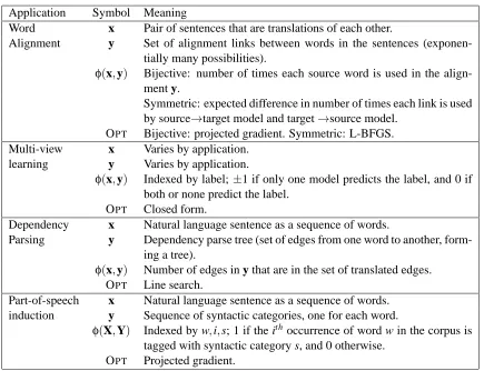
Because the PR framework allows very diverse prior information to be specified in a single formal-ism, the application Sections (§5-§8) are very diverse in nature. This section attempts to summarize their similarities and differences without getting into the details of the problem applications and intuition behind the constraints. Table 2 summarizes the applications and constraints described in the rest of the paper while Table 3 summarizes the meanings of the variables x, y andφ(X,Y)as well as the optimization procedures used for the applications presented in the sequel.
In the statistical word alignment application described in Section 5, the goal is to identify pairs or sets of words that are direct translations of each other. The statistical models used suffer from what
Application Symbol Meaning
Word x Pair of sentences that are translations of each other.
Alignment y Set of alignment links between words in the sentences (exponen-tially many possibilities).
φ(x,y) Bijective: number of times each source word is used in the align-ment y.
Symmetric: expected difference in number of times each link is used by source→target model and target→source model.
OPT Bijective: projected gradient. Symmetric: L-BFGS. Multi-view x Varies by application.
learning y Varies by application.
φ(x,y) Indexed by label;±1 if only one model predicts the label, and 0 if both or none predict the label.
OPT Closed form.
Dependency x Natural language sentence as a sequence of words.
Parsing y Dependency parse tree (set of edges from one word to another, form-ing a tree).
φ(x,y) Number of edges in y that are in the set of translated edges. OPT Line search.
Part-of-speech x Natural language sentence as a sequence of words. induction y Sequence of syntactic categories, one for each word.
φ(X,Y) Indexed by w,i,s; 1 if the ith occurrence of word w in the corpus is tagged with syntactic category s, and 0 otherwise.
OPT Projected gradient.
Table 3: Summary of input and output variable meanings as well as meanings of constraint features and optimization methods used (OPT) for the applications summarized in Table 2.
is known as a garbage collector effect: the likelihood function of the simplistic translation models used prefers to align sections that are not literal translations to rare words, rather than leaving them unaligned (Brown et al., 1993). This results in each rare word in a source language being aligned to 4 or 5 words in the target language. To alleviate this problem, we introduce constraint features that count how many target words are aligned to each source word, and use PR to encourage models where this number is small in expectation. Modifying the model itself to include such a preference would break independence and make it intractable.
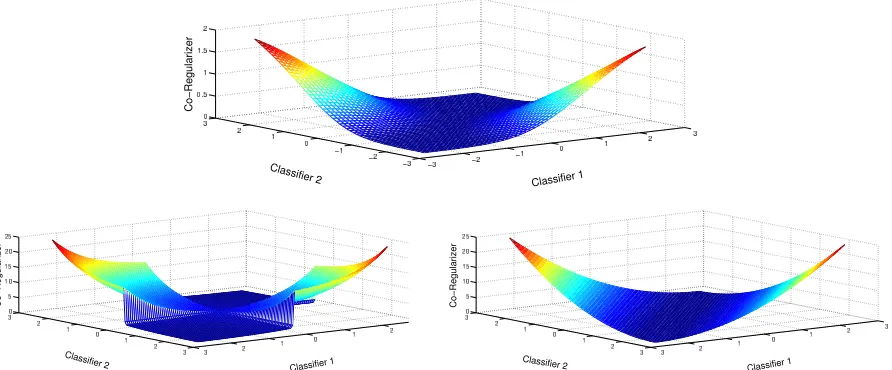
The multi-view learning application described in Section 6 leverages two or more sources of input (“views”) along with unlabeled data. The requirement is to train two models, one for each view, such that they usually agree on the labeling of the unlabeled data. We can do this using PR, and we recover the Bhattacharyya distance as a regularizer. The PR approach also extends naturally to structured problems, and cases where we only want partial agreement.
achieved using PR constraints that guide learning to prefer models that tend to agree with the noisy labeling wherever it is provided, while standard regularization guides learning to be self-consistent. Finally, Section 8 describes an application of PR to ensure a particular sparsity structure, which can be independent of the structure of the model. Section 8 focuses on the problem of unsuper-vised part-of-speech induction, where we are given a sample of text and are required to specify a syntactic category for each token in the text. A well-known but difficult to capture piece of prior knowledge for this problem is that each word type should only occur with a small number of syn-tactic categories, even though there are some synsyn-tactic categories that occur with many different word types. By using anℓ1/ℓ∞norm on constraint features we are able to encourage the model to have precisely this kind of sparsity structure, and greatly increase agreement with human-generated syntactic categories.
Table 2 also shows for each application whether we use the distribution over hidden variables given by the model parameters pθ(Y|X)to decode, or whether we first project the distribution to the constraint set and use q(Y)to decode. In general we found that when applying the constraints on the labeled data is sensible, performing the projection before decoding tends to improve performance. For the word alignment application and the multi-view learning application we found decoding with the projected distribution improved performance. By contrast, for dependency parsing, we do not have the English translations at test time and so we cannot perform a projection. For part-of-speech induction the constraints are over the entire corpus, and different regularization strengths might be needed for the training and test sets. Since we did not want to tune a second hyperparameter, we instead decoded with p.
4. Related Frameworks
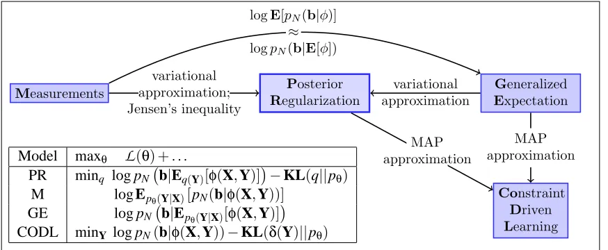
The work related to learning with constraints on posterior distributions is described in chronological order in the following three subsections. An overall summary is most easily understood in reverse chronological order though, so we begin with a few sentences detailing the connections to it in that order. Liang et al. (2009) describe how we can view constraints on posterior distributions as mea-surements in a Bayesian setting, and note that inference using such information is intractable. By approximating this problem, we recover either the generalized expectation constraints framework of Mann and McCallum (2007), or with a further approximation we recover a special case of the pos-terior regularization framework presented in Section 2. Finally, a different approximation recovers the constraint driven learning framework of Chang et al. (2007). To the best of our knowledge, we are the first to describe all these connections.
4.1 Constraint Driven Learning
Chang et al. (2007, 2008) describe a framework called constraint driven learning (CODL) that can be viewed as an approximation to optimizing the slack-penalized version of the PR objective (Equa-tion 3). Chang et al. (2007) are motivated by hard-EM, where the distribu(Equa-tion q is approximated by a single sample at the mode of log pθ(Y|X). Chang et al. (2007) propose to augment log pθ(Y|X) by adding to it a penalty term based on some domain knowledge. When the penalty terms are well-behaved, we can view them as adding a cost for violating expectations of constraint featuresφ. In such a case, CODL can be viewed as a “hard” approximation to the PR objective:
arg max
θ
L
(θ) −minq∈M
KL(q(Y)||pθ(Y|X)) + σ
Eq[φ(X,Y)]−b β
where M is the set of distributions concentrated on a single Y. The modified E-Step becomes:
CODL E′-step : max
Y log pθ(Y|X) − σ||φ(X,Y)−b||β.
Because the constraints used by Chang et al. (2007) do not allow tractable inference, they use a beam search procedure to optimize the min-KL problem. Additionally they consider a K-best variant where instead of restricting themselves to a single point estimate for q, they use a uniform distribution over the top K samples.
Carlson et al. (2010) train several named entity and relation extractors concurrently in order to satisfy type constraints and mutual exclusion constraints. Their algorithm is related to CODL in that hard assignments are made in a way that guarantees the constraints are satisfied. However, their algorithm is motivated by adding these constraints to algorithms that learn pattern extractors: at each iteration, they make assignments only to the highest confidence entities, which are then used to extract high confidence patterns for use in subsequent iterations. By contrast hard EM and CODL would make assignments to every instance and change these assignments over time. Daumé III (2008) also use constraints to filter out examples for self-training and also do not change the labels.
4.2 Generalized Expectation Criteria
Generalized expectation criteria (GE) allow a user to specify preferences about model expectations in the form of linear constraints on some feature expectations (Mann and McCallum, 2007, 2008). As with PR, a set of constraint featuresφare introduced, and a penalty term is added to the log-likelihood objective. The GE objective is
max
θ
L
(θ)−σ||Epθ[φ(X,Y)]−b||β. (15) where ||·||β is typically the l2 norm (Druck et al., 2009 use l22) or a distance based on KL diver-gence (Mann and McCallum, 2008), and the model is a log-linear model such as maximum entropy or a CRF.The idea leading to this objective is the following: Suppose that we only had enough resources to make a very small number of measurements when collecting statistics about the true distribution
p∗(y|x). If we try to create a maximum entropy model using these statistics we will end up with a very impoverished model. It will only use a small number of features and consequently will fail to generalize to instances where these features cannot occur. In order to train a more feature-rich model, GE defines a wider set of model features f and uses the small number of estimates based on constraint featuresφto guide learning. By using l2regularization on model parameters, we can ensure that a richer set of model features are used to explain the desired expectations.
Druck et al. (2009) use a gradient ascent method to optimize the objective. Unfortunately, because the second term in the GE objective (Equation 15) couples the constraint featuresφand the model parametersθ, the gradient requires computing the covariance between model features f and the constraint featuresφunder pθ:
∂Epθ[φ(X,Y)]
∂θ =Epθ[f(X,Y)φ(X,Y)]−Epθ[φ(X,Y)]Epθ[f(X,Y)].
where f and φhave the same Markov dependencies, computing this gradient usually squares the running time of the dynamic program. A more efficient dynamic program might be possible (Li and Eisner, 2009; Pauls et al., 2009), however current implementations are prohibitively slower than PR when there are many constraint features.
In order to avoid the costly optimization procedure described above, Bellare et al. (2009) pro-pose a variational approximation. Recall that at a high level, the difficulty in optimizing Equa-tion 15 is because the last term couples the constraint features φ with the model parameters θ. In order to separate out these quantities, Bellare et al. (2009) introduce an auxiliary distribution
q(Y)≈pθ(Y|X), which is used to approximate the last term in Equation 15. The variational objec-tive contains three terms instead of two:
arg max
θ
L
(θ) −minq
KL(q(Y)||pθ(Y|X)) + σ
Eq[φ(X,Y)]−b β
. (16)
This formulation is identical to the slack-penalized version of PR, and Bellare et al. (2009) use the same optimization procedure (described in Section 2). Because both the minorization and the maximization steps implement minimum Kullback-Leibler projections, Bellare et al. (2009) refer to this algorithm as alternating projections. Note that PR can also be trained in an online fashion, and Ganchev et al. (2009) use an online optimization for this objective to train a dependency parser. These experiments are described in Section 7.
Closely related to GE, is the work of Quadrianto et al. (2009). The authors describe a setting where the constraint values, b, are chosen as the empirical estimates on some labeled data. They then train a model to have high likelihood on the labeled data, but also match the constraint features on unlabeled data. They show that for appropriately chosen constraint features, the estimated constraint values should be close to the true means, and show good experimental improvements on an image retrieval task.
4.3 Measurements in a Bayesian Framework
Liang et al. (2009) approach the problem of incorporating prior information about model posteriors from a Bayesian point of view. They motivate their approach using the following caricature. Sup-pose we have log-linear model pθ(y|x)∝exp(θ·f(y,x)). In addition to any labeled data(XL,YL), we also have performed some additional experiments.7 In particular, we have observed the expected values of some constraint featuresφ(X,Y)on some unlabeled data X. Because there is error in mea-surement, they observe b≈φ(X,Y). Figure 3 illustrates this setting. The leftmost nodes represent (x,y)pairs from the labeled data(XL,YL). The nodes directly to the right ofθrepresent unlabeled
(x,y)pairs from the unlabeled data X. All the data are tied together by the dependence on the model parametersθ. The constraint features take as input the unlabeled data set X as well as a full labeling Y, and produce some valueφ(X,Y), which is never observed directly. Instead, we observe some noisy version b≈φ(X,Y). The measured values b are distributed according to some noise model
pN(b|φ(X,Y)). Liang et al. (2009) note that the optimization is convex for log-concave noise and use box noise in their experiments, giving b uniform probability in some range nearφ(X,Y).
In the Bayesian setting, the model parameters θas well as the observed measurement values b are random variables. Liang et al. (2009) use the mode of p(θ|XL,YL,X,b)as a point estimate
XL θ X
YL Y
φ(X,Y)
b
Figure 3: The model used by Liang et al. (2009), using our notation. We have separated treatment of the labeled data(XL,YL)from treatment of the unlabeled data X.
forθ:
arg max
θ p(θ|XL,YL,X,b) = arg maxθ
∑
Yp(θ,Y,b|X,XL,YL),
with equality because p(θ|XL,YL,X,b)∝p(θ,b|XL,YL,X) =∑Yp(θ,Y,b|X,XL,YL). Liang et al. (2009) focus on computing p(θ,Y,b|X,XL,YL). They define their model for this quantity as fol-lows:
p(θ,Y,b|X,XL,YL) = p(θ|XL,YL) pθ(Y|X) pN(b|φ(X,Y)) (17) where the Y and X are particular instantiations of the random variables in the entire unlabeled corpus X. Equation 17 is a product of three terms: a prior onθ, the model probability pθ(Y|X), and a noise model pN(b|φ). The noise model is the probability that we observe a value, b, of the measurement featuresφ, given that its actual value wasφ(X,Y). The idea is that we model errors in the estimation of the posterior probabilities as noise in the measurement process. Liang et al. (2009) use a uniform distribution overφ(X,Y)±ε, which they call “box noise”. Under this model, observing b farther thanεfromφ(X,Y)has zero probability. In log space, the exact MAP objective, becomes:
max
θ
L
(θ) +log Epθ(Y|X)h
pN(b|φ(X,Y))
i
. (18)
Unfortunately with almost all noise models (including no noise), and box noise in particular, the second term in Equation 18 makes the optimization problem intractable.8 Liang et al. (2009) use a variational approximation as well as a further approximation based on Jensen’s inequality to reach the PR objective, which they ultimately optimize for their experiments. We also relate their frame-work to GE and CODL. If we approximate the last term in Equation 18 by moving the expectation inside the probability:
Epθ(Y|X)
h
pN(b|φ(X,Y))
i
≈pN
b|Epθ(Y|X)[φ(X,Y)]
,
we end up with an objective equivalent to GE for appropriate noise models. In particular Gaus-sian noise corresponds to l22regularization in GE, since the log of a Gaussian is squared Euclidean distance (up to scaling). This approximation can be motivated by the case when pθ(Y|X) is con-centrated on a particular labeling Y∗: pθ(Y|X) =δ(Y∗). In this special case the≈is an equality. 8. For very special noise, such as noise that completely obscures the signal, we can compute the second term in
Measurements Posterior
Regularization
Generalized
Expectation
Constraint
Driven
Learning
variational approximation; Jensen’s inequality
variational approximation
MAP approximation MAP
approximation logE[pN(b|φ)]
≈
logpN(b|E[φ])
Model maxθ
L
(θ) +. . .PR minq log pN b|Eq(Y)[φ(X,Y)]
−KL(q||pθ) M log Epθ(Y|X)[pN(b|φ(X,Y))]
GE log pN b|Epθ(Y|X)[φ(X,Y)]
CODL minY log pN(b|φ(X,Y))−KL(δ(Y)||pθ)
Figure 4: A summary of the different models. We use pθ(Y|X) to denote the model probability,
q(Y) to denote a proposal distribution, and pN for the noise model. The symbolδ(Y) denotes a distribution concentrated on Y. The approximations are described in the text: M→GE near Equation 19, GE→PR near Equation 16, PR→CODL at the end of Sec-tion 4.3.
This approximation is also used in Liang et al. (2009). This provides an interpretation of GE as an approximation to the Bayesian framework proposed by Liang et al. (2009):
max
θ
L
(θ) +log pN
b Epθ(Y|X)[φ(X,Y)]
. (19)
Note that the objective in Equation 19 is a reasonable objective in and of itself, essentially stating that the measured values b are not dependent on any particular instantiation of the hidden variables, but rather represent the integral over all their possible assignments. Liang et al. (2009) also use a variational approximation similar to the one of Bellare et al. (2009) so that the objective they optimize is exactly the PR objective, although their optimization algorithm is slightly different from the one presented in Section 2. Finally, if we restrict the set of allowable distributions further to be concentrated on a single labeling Y, we recover the CODL algorithm. Figure 4 summarizes the relationships.
5. Statistical Word Alignments
Word alignments, introduced by Brown et al. (1994) as hidden variables in probabilistic models for statistical machine translation (IBM models 1-5), describe the correspondence between words in source and target sentences. We will denote each target sentence as xt= (xt
1, . . . ,xti, . . . ,xtI)and each source sentence as xs= (xs1, . . . ,xsj, . . . ,xs
and rules in syntax-based machine translation (Galley et al., 2004; Chiang et al., 2005), as well as for MT system combination (Matusov et al., 2006). But their importance has grown far beyond machine translation: for instance, transferring annotations between languages by projecting POS taggers, NP chunkers and parsers through word alignment (Yarowsky and Ngai, 2001; Rogati et al., 2003; Hwa et al., 2005; Ganchev et al., 2009); discovery of paraphrases (Bannard and Callison-Burch, 2005; Callison-Callison-Burch, 2007, 2008); and joint unsupervised POS and parser induction across languages (Snyder and Barzilay, 2008; Snyder et al., 2009).
Here we describe two types of prior knowledge that when introduced as constraints in different word alignment models significantly boost their performance. The two constraints are: (i) bijec-tivity: “one word should not translate to many words”; and (ii) symmetry: “directional alignments of one model should agree with those of another model”. A more extensive description of these constraints applied to the task of word alignments and the quality of the resulting alignments can be found in Graça et al. (2010).
5.1 Models
We consider two models below: IBM Model 1 proposed by Brown et al. (1994) and the HMM model proposed by Vogel et al. (1996). Both models can be expressed as:
p(xt,y|xs) =
∏
j
pd(yj| j,yj−1)pt(xtj|xsyj),
where y is the alignment and yj is the index of the hidden state (source language index) generating the target language word at index j. The models differ in their definition of the distortion probability
pd(yj | j,yj−1). Model 1 assumes that the target words are generated independently and assigns uniform distortion probability. The HMM model assumes that only the distance between the current and previous source word index is important pd(yj| j,yj−1) =pd(yj |yj−yj−1). Both models are augmented by adding a special “null” word to the source sentence.
The likelihood of the corpus, marginalized over possible alignments, is concave for Model 1, but not for the HMM model (Brown et al., 1994; Vogel et al., 1996). For both models though, stan-dard training using the Expectation Maximization algorithm (Dempster et al., 1977) seeks model parametersθthat maximize the log-likelihood of the parallel corpus.
On the positive side, both models are simple and complexity of inference is O(I×J)for IBM Model 1 and O(I×J2)for the HMM. However there are several problems with the models that arise from their directionality.
• Non-bijective: Multiple target words can align to a single source word with no penalty.
• Asymmetric: Swapping the source and target languages can produce very different align-ments, since only constraints and correlations between consecutive positions on one side are enforced by the models.
0 1 2 3 4 5 6 7 8 9 0 1 2 3 4 5 6 7 8 9
0 p p p p p p p p p p 0 p p p p z p p p p p instead
1 p p p p p p p p p p 1 p p p p p z p p p p of
2 p p p p p p p p p p 2 p p p p p p z p p p causing
3 p p p p p p p p p p 3 p p p p p p s p u p an
4 p p p v p p p p p p 4 p p p p p p p p z p internal
5 x x x p z p z w z p 5 p p p p p p p p z p schism
6 p p p p p p p p p z 6 p p p p p p p p p z ,
0 1 2 3 4 5 6 7 8 9 0 1 2 3 4 5 6 7 8 9
0 p p p p z p p p p p 0 p p p p z p p p p p instead
1 p p p p p v p p p p 1 p p p p p y p p p p of
2 p p p p p p z p p p 2 p p p p p p z p p p causing
3 p p p p p p p x p p 3 p p p p p p p w p p an
4 p p p p p p p p p p 4 p p p z p p p p p p internal
5 p p p p p p p p z p 5 p p p p p p p p z p schism
6 p p p p p p p p p x 6 p p p p p p p p p z ,
0 1 2 3 4 5 6 7 8 9 0 1 2 3 4 5 6 7 8 9
0 p p p p z p p p p p 0 p p p p z p p p p p instead
1 p p p p p z p p p p 1 p p p p p z p p p p of
2 p p p p p p z p p p 2 p p p p p p z p p p causing
3 p q q p p p p w p p 3 p q q p p p p w p p an
4 p p p x p p p p p p 4 p p p x p p p p p p internal
5 p p p p p p p p z p 5 p p p p p p p p z p schism
6 p p p p p p p p p z 6 p p p p p p p p p z ,
et que à le lie
u de prov oque
r la ruptur
e
, et que à le lie
u de prov oque
r la ruptur
e ,
Figure 5: Posterior distributions on an English to French sentence using the HMM model. Left: EN→FR model. Right: FR→EN model. Top: Regular EM posteriors. Middle: After applying bijective constraint. Bottom: After applying symmetric constraint. Sure align-ments are squares with borders; possible alignalign-ments are squares without borders. Circle size indicates probability value. See Graça et al. (2010) for a description of the difference between sure and possible alignments. Circle color in the middle and bottom rows indi-cates difference in posterior from the top row. Green (light gray) - higher probability, red (dark gray) - lower probability.
occurring less than 5 times in the corpus) in both directions, instead of being spread across differ-ent words. This is a well known problem when training using EM, called the “garbage collector effect” (Brown et al., 1993). That is, rare words in the source language end up aligned to too many words in the target language because the generative model has to distribute translation probability for each source word among all candidate target words. Since the rare source word occurs in only a few sentences it needs to spread its probability mass over fewer competing target words. In this case, choosing to align the rare word to all of these target words leads to higher likelihood than correctly aligning them or aligning them to the special null word, since it increases the likelihood of this sentence without lowering the likelihood of many other sentences. Moreover, by correcting the garbage collector effect we increase the overall performance on the common words, since now these common words can be aligned to the correct words. For this particular corpus, 6.5% of the English tokens and 7.7% of the French tokens are rare.
5.2 Bijectivity Constraints
trend into the model, but adding it directly requires large factors (breaking the Markov property). In fact, summing over one-to-one or near one-to-one weighted matchings is a classical #P-Complete problem (Valiant, 1979). However, introducing alignment degree constraints in expectation in the PR framework is easy and tractable. We simply add inequality constraints E[φ(x,y)]≤1 where we have one feature for each source word j that counts how many times it is aligned to a target word in the alignment y:
Bijective Features : φj(x,y) =
∑
i1(yi= j).
For example, in the alignment at the top right of Figure 5, the posteriors over the source word
schism clearly sum to more than 1. The effect of applying PR constraints to the posteriors is shown in
the second row. Enforcing the one to (at most) one constraint clearly alleviates the garbage collector effect. Moreover, when distributing the probability mass to the other words, most of the probability mass goes into the correct positions (as can be seen by comparison to the gold alignments). Note that the bijectivity constraints only hold approximately in practice and so we expect that having a KL-based penalty for them might be better than ensuring that the model satisfies them, since we can violate bijectivity in order to achieve higher likelihood. Another way to understand what is going on is to see how the parameters are affected by the bijectivity constraint. In particular the translation table becomes much cleaner, having a much lower entropy. The average entropy for the translation probability, averaged over all source language words for EM training is 2.0-2.6 bits, depending on the direction. When we train using PR with the bijectivity constraint, this entropy drops to 0.6 for both directions. We see that while the model does not have any particular parameter that can enforce bijectivity, in practice the model is expressive enough to learn a preference for bijectivity by appropriately setting the existing model parameters.
5.3 Symmetry Constraints
Word alignment should not depend on translation direction, but this principle is clearly violated by the directional models. In fact, each directional model makes different mistakes. The standard approach is to train two models independently and then intersect their predictions (Och and Ney, 2003).9 However, we show that it is much better to train two directional models concurrently, cou-pling their posterior distributions over alignments with constraints that force them to approximately agree. The idea of training jointly has also been explored by Matusov et al. (2004) and Liang et al. (2006), although their formalization is quite different.
Let the directional models be defined as: −→pθ(−→y)(forward) and←−pθ(←−y)(backward). We sup-press dependence on xsand xt for brevity. Define y to range over the union of all possible directional alignments−→y ∪ ←−y . We then define a mixture model pθ(y) =1
2 − →p
θ(y) +12 ←−p
θ(y)where←−pθ(−→y) =0 and vice-versa (i.e., the alignment of one directional model has probability zero according to the other model). We then define the following feature for each target-source position pair i,j:
Symmetric Features : φi j(x,y) =
+1 y∈ −→y and−→yi = j −1 y∈ ←−y and←y−j =i 0 otherwise.
The feature takes the value zero in expectation if a word pair i,j is aligned with equal probability in
both directions. So the constraint we want to impose is Eq[φi j(x,y)] =0 (possibly with some small
violation). Note that this constraint is only feasible if the posteriors are bijective. Clearly these features are fully factored, so to compute expectations of these features under the model q we only need to be able to compute them under each directional model, as we show below. To see this, we have by the definition of qλand pθ,
qλ(y|x) =
− →p
θ(y|x) +←−pθ(y|x) 2
exp{−λ·φ(x,y)}
Z =
−
→q(y|x) Z−→q
− →p
θ(x)+
←−q(y|x) Z←−q
←−p θ(x)
2Z ,
where we have defined:
−
→q(y|x) = 1
Z−→q − →p
θ(y,x)exp{−λ·φ(x,y)} with Z−→q =
∑
y
− →p
θ(y,x)exp{−λ·φ(x,y)}, ←−q(y|x) = 1
Z←−q ←−p
θ(y,x)exp{−λ·φ(x,y)} with Z←−q =
∑
y
←−p
θ(y,x)exp{−λ·φ(x,y)},
Z= 1
2
Z−→q − →p
θ(x)+
Z←−q ←−p
θ(x)
!
.
All these quantities can be computed separately in each model.
The last row in Figure 5 shows both directional posteriors after imposing the symmetric con-straint. Note that the projected posteriors are equal in the two models. Also, one can see that in most cases the probability mass was moved to the correct place with the exception of the word pair
inter-nal/le; this is because the word internal does not appear on the French side, but the model still has
to spread around the probability mass for that word. In this case the model decided to accumulate it on the word le instead of moving it to the null word.
5.4 Algorithm for Projection
Because both the symmetric and bijective constraints decompose over sentences, and the model distribution p(Y|X)decomposes as a product distribution over instances, the projected distribution
q(Y) will also decompose as a product over instances. Furthermore, because the constraints for different instances do not interact, we can project the sentences one at a time and we do not need to store the posteriors for the whole corpus in memory at once. We compute q(y)for each sentence pair x using projected gradient ascent for the bijective constraints and L-BFGS for the symmetric constraints.
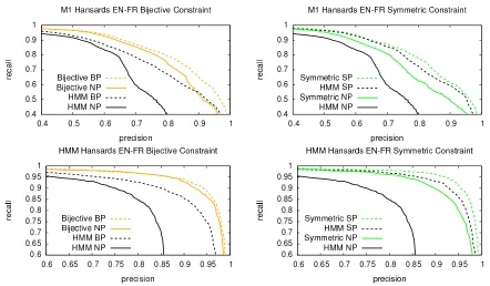
5.5 Results
Figure 6: Precision vs Recall curves of both models using standard EM training (Regular) versus PR with bijective constraints (Bijective) and symmetry constraints (Symmetric) and dif-ferent decoding types: decoding without any projection (NP), doing bijective projection before decoding (BP), and doing symmetric projection before decoding (SP). Data is 100k sentences of the Hansard corpus. Highest label in the legend corresponds to highest line in the graph, second highest label to second highest line, and so on.
Figure 6 shows the precision vs recall curves of both models (EN-FR, FR-EN independently) when training using standard EM versus PR with both constraints, and the results of additionally applying the constraints at decode time in order to tease apart the effect of the constraints during training vs. during testing. The first observation is that training with PR significantly boosts the performance of each model. Moreover using the projection at decode time always increases perfor-mance. Comparing both constraints, it seems that the bijective constraint is more useful at training time. Note that using this constraint at decode time with regular training yields worse results than just training with the same constraint using PR. On the other hand, the symmetric constraint is stronger at decode time.