Hubs in Space: Popular Nearest Neighbors in High-Dimensional Data

Hubs in Space: Popular Nearest Neighbors in High-Dimensional Data

Miloˇs Radovanovi´c [email protected]

Department of Mathematics and Informatics University of Novi Sad

Trg D. Obradovi´ca 4, 21000 Novi Sad, Serbia

Alexandros Nanopoulos [email protected]

Institute of Computer Science University of Hildesheim

Marienburger Platz 22, D-31141 Hildesheim, Germany

Mirjana Ivanovi´c [email protected]

Department of Mathematics and Informatics University of Novi Sad

Trg D. Obradovi´ca 4, 21000 Novi Sad, Serbia

Editor: Ulrike von Luxburg

Abstract

Different aspects of the curse of dimensionality are known to present serious challenges to various machine-learning methods and tasks. This paper explores a new aspect of the dimensionality curse, referred to as hubness, that affects the distribution of k-occurrences: the number of times a point appears among the k nearest neighbors of other points in a data set. Through theoretical and empir-ical analysis involving synthetic and real data sets we show that under commonly used assumptions this distribution becomes considerably skewed as dimensionality increases, causing the emergence of hubs, that is, points with very high k-occurrences which effectively represent “popular” nearest neighbors. We examine the origins of this phenomenon, showing that it is an inherent property of data distributions in high-dimensional vector space, discuss its interaction with dimensionality reduction, and explore its influence on a wide range of machine-learning tasks directly or indi-rectly based on measuring distances, belonging to supervised, semi-supervised, and unsupervised learning families.

Keywords: nearest neighbors, curse of dimensionality, classification, semi-supervised learning,

clustering

1. Introduction

The curse of dimensionality, a term originally introduced by Bellman (1961), is nowadays com-monly used in many fields to refer to challenges posed by high dimensionality of data space. In the field of machine learning, affected methods and tasks include Bayesian modeling (Bishop, 2006), nearest-neighbor prediction (Hastie et al., 2009) and search (Korn et al., 2001), neural networks (Bishop, 1996), and many others. One aspect of the dimensionality curse is distance concentration, which denotes the tendency of distances between all pairs of points in high-dimensional data to become almost equal. Distance concentration and the meaningfulness of nearest neighbors in high

dimensions has been thoroughly explored (Beyer et al., 1999; Hinneburg et al., 2000; Aggarwal et al., 2001; Franc¸ois et al., 2007). The effect of the phenomenon on machine learning was demon-strated, for example, in studies of the behavior of kernels in the context of support vector machines, lazy learning, and radial basis function networks (Evangelista et al., 2006; Franc¸ois, 2007).

There exists another aspect of the curse of dimensionality that is related to nearest neigh-bors (NNs), which we will refer to as hubness. Let D_⊂Rd _{be a set of d-dimensional points} and Nk(x)the number of k-occurrences of each point x∈D, that is, the number of times x occurs among the k nearest neighbors of all other points in D, according to some distance measure. Under widely applicable conditions, as dimensionality increases, the distribution of Nkbecomes consider-ably skewed to the right, resulting in the emergence of hubs, that is, points which appear in many more k-NN lists than other points, effectively making them “popular” nearest neighbors. Unlike distance concentration, hubness and its influence on machine learning have not been explored in depth. In this paper we study the causes and implications of this aspect of the dimensionality curse. As will be described in Section 4, the phenomena of distance concentration and hubness are related, but distinct. Traditionally, distance concentration is studied through asymptotic behavior of norms, that is, distances to the origin, with increasing dimensionality. The obtained results trivially extend to reference points other than the origin, and to pairwise distances between all points. However, the asymptotic tendencies of distances of all points to different reference points do not necessarily occur at the same speed, which will be shown for normally distributed data by our main theoretical result outlined in Section 4.2, and given with full details in Section 5.1. The main consequence of the analysis, which is further discussed in Section 5.2 and supported by theoretical results by Newman et al. (1983) and Newman and Rinott (1985), is that the hubness phenomenon is an inherent property of data distributions in high-dimensional space under widely used assumptions, and not an artefact of a finite sample or specific properties of a particular data set.

The above result is relevant to machine learning because many families of ML algorithms, regardless of whether they are supervised, semi-supervised, or unsupervised, directly or indirectly make use of distances between data points (and, with them, k-NN graphs) in the process of building a model. Moreover, the hubness phenomenon recently started to be observed in application fields like music retrieval (Aucouturier and Pachet, 2007), speech recognition (Doddington et al., 1998), and fingerprint identification (Hicklin et al., 2005), where it is described as a problematic situation, but little or no insight is offered into the origins of the phenomenon. In this paper we present a unifying view of the hubness phenomenon through theoretical analysis of data distributions, and empirical investigation including numerous synthetic and real data sets, explaining the origins of the phenomenon and the mechanism through which hubs emerge, discussing the role of antihubs (points which appear in very few, if any, k-NN lists of other points), and studying the effects on common supervised, semi-supervised, and unsupervised machine-learning algorithms.

previ-ously established link between intrinsic dimensionality and hubness, and demonstrating that dimen-sionality reduction may not constitute an easy mitigation of the phenomenon. Section 7 explores the impact of hubness on common supervised, semi-supervised, and unsupervised machine-learning algorithms, showing that the information provided by hubness can be used to significantly affect the success of the generated models. Finally, Section 8 concludes the paper, and provides guidelines for future work.

2. Related Work

The hubness phenomenon has been recently observed in several application areas involving sound and image data (Aucouturier and Pachet, 2007; Doddington et al., 1998; Hicklin et al., 2005). Also, Jebara et al. (2009) briefly mention hubness in the context of graph construction for semi-supervised learning. In addition, there have been attempts to avoid the influence of hubs in 1-NN time-series classification, apparently without clear awareness about the existence of the phenomenon (Islam et al., 2008), and to account for possible skewness of the distribution of N1 in reverse nearest-neighbor search (Singh et al., 2003),1 where Nk(x) denotes the number of times point x occurs among the k nearest neighbors of all other points in the data set. None of the mentioned papers, however, successfully analyze the causes of hubness or generalize it to other applications. One recent work that makes the connection between hubness and dimensionality is the thesis by Beren-zweig (2007), who observed the hubness phenomenon in the application area of music retrieval and identified high dimensionality as a cause, but did not provide practical or theoretical support that would explain the mechanism through which high dimensionality causes hubness in music data.

The distribution of N1 has been explicitly studied in the applied probability community (New-man et al., 1983; Maloney, 1983; New(New-man and Rinott, 1985; Yao and Simons, 1996), and by math-ematical psychologists (Tversky et al., 1983; Tversky and Hutchinson, 1986). In the vast majority of studied settings (for example, Poisson process, d-dimensional torus), coupled with Euclidean distance, it was shown that the distribution of N1converges to the Poisson distribution with mean 1, as the number of points n and dimensionality d go to infinity. Moreover, from the results by Yao and Simons (1996) it immediately follows that, in the Poisson process case, the distribution of Nk converges to the Poisson distribution with mean k, for any k_≥1. All these results imply that no hubness is to be expected within the settings in question. On the other hand, in the case of continu-ous distributions with i.i.d. components, for the following specific order of limits it was shown that limn_→∞limd_→∞Var(N1) =∞, while limn_→∞limd_→∞N1=0, in distribution (Newman et al., 1983, p. 730, Theorem 7), with a more general result provided by Newman and Rinott (1985). Accord-ing to the interpretation by Tversky et al. (1983), this suggests that if the number of dimensions is large relative to the number of points one may expect a small proportion of points to become hubs. However, the importance of this finding was downplayed to a certain extent (Tversky et al., 1983; Newman and Rinott, 1985), citing empirically observed slow convergence (Maloney, 1983), with the attention of the authors shifting more towards similarity measurements obtained directly from psychological and cognitive experiments (Tversky et al., 1983; Tversky and Hutchinson, 1986) that do not involve vector-space data. In Section 5.2 we will discuss the above results in more detail, as well as their relations with our theoretical and empirical findings.

It is worth noting that inε-neighborhood graphs, that is, graphs where two points are connected if the distance between them is less than a given limitε, the hubness phenomenon does not occur.

Settings involving randomly generated points formingε-neighborhood graphs are typically referred to as random geometric graphs, and are discussed in detail by Penrose (2003).

Concentration of distances, a phenomenon related to hubness, was studied for general distance measures (Beyer et al., 1999; Durrant and Kab´an, 2009) and specifically for Minkowski and frac-tional distances (Demartines, 1994; Hinneburg et al., 2000; Aggarwal et al., 2001; Franc¸ois et al., 2007; Franc¸ois, 2007; Hsu and Chen, 2009). Concentration of cosine similarity was explored by Nanopoulos et al. (2009).

In our recent work (Radovanovi´c et al., 2009), we performed an empirical analysis of hubness, its causes, and effects on techniques for classification, clustering, and information retrieval. In this paper we extend our findings with additional theoretical and empirical insight, offering a unified view of the origins and mechanics of the phenomenon, and its significance to various machine-learning applications.

3. The Hubness Phenomenon

In Section 1 we gave a simple set-based deterministic definition of Nk. To complement this definition and introduce Nkinto a probabilistic setting that will also be considered in this paper, let x,x1, . . . ,xn, be n+1 random vectors drawn from the same continuous probability distribution with support

S

pi,k(x) =

1, if x is among the k nearest neighbors of xi, according to dist, 0, otherwise.

In this setting, we define Nk(x) =∑ni=1pi,k(x), that is, Nk(x)is the random number of vectors from Rd _{that have x included in their list of k nearest neighbors. In this section we will empirically} demonstrate the emergence of hubness through increasing skewness of the distribution of Nk on synthetic (Section 3.1) and real data (Section 3.2), relating the increase of skewness with the di-mensionality of data sets, and motivating the subsequent study into the origins of the phenomenon in Section 4.

3.1 A Motivating Example

We start with an illustrative experiment which demonstrates the changes in the distribution of Nk with varying dimensionality. Let us consider a random data set consisting of 10000 d-dimensional points, whose components are independently drawn from the uniform distribution in range[0,1], and the following distance functions: Euclidean (l2), fractional l0.5(proposed for high-dimensional data by Aggarwal et al., 2001), and cosine. Figure 1(a–c) shows the empirically observed distributions of Nk, with k=5, for (a) d=3, (b) d=20, and (c) d=100. In the same way, Figure 1(d–f) depicts the empirically observed Nkfor points randomly drawn from the i.i.d. normal distribution.

For d =3 the empirical distributions of N5for the three distance functions (Figure 1(a, d)) are consistent with the binomial distribution. This is expected by considering k-occurrences as node in-degrees in the k-nearest neighbor digraph. For randomly distributed points in low dimensions, the degree distributions of the digraphs closely resemble the degree distribution of the Erd˝os-R´enyi (ER) random graph model, which is is binomial and Poisson in the limit (Erd˝os and R´enyi, 1959).

0 5 10 15 0 0.05 0.1 0.15 0.2 0.25

iid uniform, d = 3

N 5 p (N 5 ) l 2 l_0.5 cos

0 10 20 30 40 50

0 0.02 0.04 0.06 0.08 0.1 0.12 0.14 0.16

iid uniform, d = 20

N 5 p (N 5 ) l₂ l 0.5 cos

0 0.5 1 1.5 2 2.5 −4 −3.5 −3 −2.5 −2 −1.5 −1 −0.5

iid uniform, d = 100

log

10(N5)

log 10 ( p (N 5 )) l 2 l_0.5 cos

(a) (b) (c)

0 5 10 15

0 0.05 0.1 0.15 0.2 0.25

iid normal, d = 3

N 5 p (N 5 ) l 2 l 0.5 cos

0 10 20 30 40 50

0 0.05 0.1 0.15 0.2

iid normal, d = 20

N 5 p (N 5 ) l 2 l 0.5 cos

0 0.5 1 1.5 2 2.5 3 −4

−3 −2 −1 0

iid normal, d = 100

log

10(N5)

log 10 ( p (N 5 )) l 2 l 0.5 cos

(d) (e) (f)

Figure 1: Empirical distribution of N5 for Euclidean, l0.5, and cosine distances on (a–c) i.i.d.

uni-form, and (d–f) i.i.d. normal random data sets with n=10000 points and dimensionality (a, d) d=3, (b, e) d=20, and (c, f) d=100 (log-log plot).

We verified this by being able to fit major right portions (that is, tails) of the observed distributions with the log-normal distribution, which is highly skewed.2 We made similar observations with various k values (generally focusing on the common case k_≪n, where n is the number of points in a data set), distance measures (lp-norm distances for both p_≥1 and 0<p<1, Bray-Curtis, normalized Euclidean, and Canberra), and data distributions. In virtually all these cases, skewness exists and produces hubs, that is, points with high k-occurrences. One exception visible in Figure 1 is the combination of cosine distance and normally distributed data. In most practical settings, however, such situations are not expected, and a thorough discussion of the necessary conditions for hubness to occur in high dimensions will be given in Section 5.2.

3.2 Hubness in Real Data

To illustrate the hubness phenomenon on real data, let us consider the empirical distribution of Nk (k=10) for three real data sets, given in Figure 2. As in the previous section, a considerable increase in the skewness of the distributions can be observed with increasing dimensionality.

In all, we examined 50 real data sets from well known sources, belonging to three categories: UCI multidimensional data, gene expression microarray data, and textual data in the bag-of-words

2. Fits were supported by theχ2 goodness-of-fit test at 0.05 significance level, where bins represent the number of observations of individual Nkvalues. These empirical distributions were compared with the expected output of a

0 5 10 15 20 0

0.05 0.1 0.15 0.2 0.25

N

10

p

(N

10

)

haberman, d = 3

0 10 20 30 40

0 0.05 0.1 0.15 0.2 0.25

mfeat−factors, d = 216

N

10

p

(N

10

)

1 1.5 2 2.5 3

−3 −2 −1 0

log

10(N10)

log

10

(p

(N

10

))

movie−reviews, d = 11885

(a) (b) (c)

Figure 2: Empirical distribution of N10for three real data sets of different dimensionalities.

representation,3listed in Table 1. The table includes columns that describe data-set sources (2nd col-umn), basic statistics (data transformation (3rd column): whether standardization was applied, or for textual data the used bag-of-words document representation; the number of points (n, 4th column); dimensionality (d, 5th column); the number of classes (7th column)), and the distance measure used (Euclidean or cosine, 8th column). We took care to ensure that the choice of distance measure and preprocessing (transformation) corresponds to a realistic scenario for the particular data set.

To characterize the asymmetry of Nk we use the standardized third moment of the distribution of k-occurrences,

SNk=

E(Nk−µNk)

3

σ3 Nk

,

where µNkandσNkare the mean and standard deviation of Nk, respectively. The corresponding (9th)

column of Table 1, which shows the empirical SN10 values for the real data sets, indicates that the

distributions of N10 for most examined data sets are skewed to the right.4 The value of k is fixed at 10, but analogous observations can be made with other values of k.

It can be observed that some SNkvalues in Table 1 are quite high, indicating strong hubness in the

corresponding data sets.5 Moreover, computing the Spearman correlation between d and SNk over

all 50 data sets reveals it to be strong (0.62), signifying that the relationship between dimensionality and hubness extends from synthetic to real data in general. On the other hand, careful scrutiny of the charts in Figure 2 and SNk values in Table 1 reveals that for real data the impact of dimensionality

on hubness may not be as strong as could be expected after viewing hubness on synthetic data in Figure 1. Explanations for this observation will be given in the next section.

3. We used the movie review polarity data set v2.0 initially introduced by Pang and Lee (2004), while the computers and sports data sets were first used by Radovanovi´c and Ivanovi´c (2006). Preprocessing of all text data sets (except dexter, which is already preprocessed) involved stop-word removal and stemming using the Porter stemmer. Documents were transformed into the bag-of-words representation with word weights being either term frequencies (tf), or term frequencies multiplied by inverse document frequencies (tf-idf), with the choice based on independent experiments involving several classifiers. All term frequency vectors were normalized to average document length.

4. If SNk=0 there is no skewness, positive (negative) values signify skewness to the right (left).

Name Src. Trans. n d dmle Cls. Dist. SN10 S

S

N10 Clu. C

N10

dm C

N10

cm BNf10 CBNN1010 CAV

abalone UCI stan 4177 8 5.39 29 l2 0.277 0.235 62 −0.047−0.526 0.804 0.934 0.806

arcene UCI stan 100 10000 22.85 2 l2 0.634 2.639 2 −0.559−0.684 0.367 0.810 0.455

arrhythmia UCI stan 452 279 21.63 16 l2 1.984 6.769 8 −0.867−0.892 0.479 0.898 0.524

breast-w UCI stan 699 9 5.97 2 l2 1.020 0.667 7 −0.062−0.240 0.052 0.021 0.048

diabetes UCI stan 768 8 6.00 2 l2 0.555 0.486 15 −0.479−0.727 0.322 0.494 0.337

dorothea UCI none 800 100000 201.11 2 cos 2.355 1.016 19 −0.632−0.672 0.108 0.236 0.092 echocardiogram UCI stan 131 7 4.92 2 l2 0.735 0.438 5 −0.722−0.811 0.372 0.623 0.337

ecoli UCI stan 336 7 4.13 8 l2 0.116 0.208 8 −0.396−0.792 0.223 0.245 0.193

gisette UCI none 6000 5000 149.35 2 cos 1.967 4.671 76 −0.667−0.854 0.045 0.367 0.241 glass UCI stan 214 9 4.37 7 l2 0.154 0.853 11 −0.430−0.622 0.414 0.542 0.462

haberman UCI stan 306 3 2.89 2 l2 0.087−0.316 11 −0.330−0.573 0.348 0.305 0.360

ionosphere UCI stan 351 34 13.57 2 l2 1.717 2.051 18 −0.639−0.832 0.185 0.464 0.259

iris UCI stan 150 4 2.96 3 l2 0.126−0.068 4 −0.275−0.681 0.087 0.127 0.147

isolet1 UCI stan 1560 617 13.72 26 l2 1.125 6.483 38 −0.306−0.760 0.283 0.463 0.352

mfeat-factors UCI stan 2000 216 8.47 10 l2 0.826 5.493 44 −0.113−0.688 0.063 0.001 0.145

mfeat-fourier UCI stan 2000 76 11.48 10 l2 1.277 4.001 44 −0.350−0.596 0.272 0.436 0.415

mfeat-karhunen UCI stan 2000 64 11.82 10 l2 1.250 8.671 40 −0.436−0.788 0.098 0.325 0.205

mfeat-morph UCI stan 2000 6 3.22 10 l2 −0.153 0.010 44 −0.039−0.424 0.324 0.306 0.397

mfeat-pixel UCI stan 2000 240 11.83 10 l2 1.035 3.125 44 −0.210−0.738 0.049 0.085 0.107

mfeat-zernike UCI stan 2000 47 7.66 10 l2 0.933 3.389 44 −0.185−0.657 0.235 0.252 0.400

musk1 UCI stan 476 166 6.74 2 l2 1.327 3.845 17 −0.376−0.752 0.237 0.621 0.474

optdigits UCI stan 5620 64 9.62 10 l2 1.095 3.789 74 −0.223−0.601 0.044 0.097 0.168

ozone-eighthr UCI stan 2534 72 12.92 2 l2 2.251 4.443 49 −0.216−0.655 0.086 0.300 0.138

ozone-onehr UCI stan 2536 72 12.92 2 l2 2.260 5.798 49 −0.215−0.651 0.046 0.238 0.070

page-blocks UCI stan 5473 10 3.73 5 l2 −0.014 0.470 72 −0.063−0.289 0.049−0.046 0.068

parkinsons UCI stan 195 22 4.36 2 l2 0.729 1.964 8 −0.414−0.649 0.166 0.321 0.256

pendigits UCI stan 10992 16 5.93 10 l2 0.435 0.982 104 −0.062−0.513 0.014−0.030 0.156

segment UCI stan 2310 19 3.93 7 l2 0.313 1.111 48 −0.077−0.453 0.089 0.074 0.332

sonar UCI stan 208 60 9.67 2 l2 1.354 3.053 8 −0.550−0.771 0.286 0.632 0.461

spambase UCI stan 4601 57 11.45 2 l2 1.916 2.292 49 −0.376−0.448 0.139 0.401 0.271

spectf UCI stan 267 44 13.83 2 l2 1.895 2.098 11 −0.616−0.729 0.300 0.595 0.366

spectrometer UCI stan 531 100 8.04 10 l2 0.591 3.123 17 −0.269−0.670 0.200 0.225 0.242

vehicle UCI stan 846 18 5.61 4 l2 0.603 1.625 25 −0.162−0.643 0.358 0.435 0.586

vowel UCI stan 990 10 2.39 11 l2 0.766 0.935 27 −0.252−0.605 0.313 0.691 0.598

wdbc UCI stan 569 30 8.26 2 l2 0.815 3.101 16 −0.449−0.708 0.065 0.170 0.129

wine UCI stan 178 13 6.69 3 l2 0.630 1.319 3 −0.589−0.874 0.076 0.182 0.084

wpbc UCI stan 198 33 8.69 2 l2 0.863 2.603 6 −0.688−0.878 0.340 0.675 0.360

yeast UCI stan 1484 8 5.42 10 l2 0.228 0.105 34 −0.421−0.715 0.527 0.650 0.570

AMLALL KR none 72 7129 31.92 2 l2 1.166 1.578 2 −0.868−0.927 0.171 0.635 0.098

colonTumor KR none 62 2000 11.22 2 l2 1.055 1.869 3 −0.815−0.781 0.305 0.779 0.359

DLBCL KR none 47 4026 16.11 2 l2 1.007 1.531 2 −0.942−0.947 0.338 0.895 0.375

lungCancer KR none 181 12533 59.66 2 l2 1.248 3.073 6 −0.537−0.673 0.052 0.262 0.136

MLL KR none 72 12582 28.42 3 l2 0.697 1.802 2 −0.794−0.924 0.211 0.533 0.148

ovarian-61902 KR none 253 15154 9.58 2 l2 0.760 3.771 10 −0.559−0.773 0.164 0.467 0.399

computers dmoz tf 697 1168 190.33 2 cos 2.061 2.267 26 −0.566−0.731 0.312 0.699 0.415 dexter UCI none 300 20000 160.78 2 cos 3.977 4.639 13 −0.760−0.781 0.301 0.688 0.423 mini-newsgroups UCI tf-idf 1999 7827 3226.43 20 cos 1.980 1.765 44 ₋0.422₋0.704 0.524 0.701 0.526 movie-reviews PaBo tf 2000 11885 54.95 2 cos 8.796 7.247 44 −0.604−0.739 0.398 0.790 0.481 reuters-transcribed UCI tf-idf 201 3029 234.68 10 cos 1.165 1.693 3 −0.781−0.763 0.642 0.871 0.595 sports dmoz tf 752 1185 250.24 2 cos 1.629 2.543 27 −0.584−0.736 0.260 0.604 0.373 Table 1: Real data sets. Data sources are the University of California, Irvine (UCI) Machine

4. The Origins of Hubness

This section moves on to exploring the causes of hubness and the mechanisms through which hubs emerge. Section 4.1 investigates the relationship between the position of a point in data space and hubness. Next, Section 4.2 explains the mechanism through which hubs emerge as points in high-dimensional space that become closer to other points than their low-dimensional counterparts, outlining our main theoretical result. The emergence of hubness in real data is studied in Section 4.3, while Section 4.4 discusses hubs and their opposites—antihubs—and the relationships between hubs, antihubs, and different notions of outliers.

4.1 The Position of Hubs

Let us consider again the i.i.d. uniform and i.i.d. normal random data examined in the previous section. We will demonstrate that the position of a point in data space has a significant effect on its k-occurrences value, by observing the sample mean of the data distribution as a point of reference. Figure 3 plots, for each point x, its N5(x) against its Euclidean distance from the empirical data mean, for d =3, 20, 100. As dimensionality increases, stronger correlation emerges, implying that points closer to the mean tend to become hubs. We made analogous observations with other values of k, and combinations of data distributions and distance measures for which hubness occurs. It is important to note that proximity to one global data-set mean correlates with hubness in high dimensions when the underlying data distribution is unimodal. For multimodal data distributions, for example those obtained through a mixture of unimodal distributions, hubs tend to appear close to the means of individual component distributions of the mixture. In the discussion that follows in Section 4.2 we will assume a unimodal data distribution, and defer the analysis of multimodal distributions until Section 4.3, which studies real data.

4.2 Mechanisms Behind Hubness

Although one may expect that some random points are closer to the data-set mean than others, in order to explain the mechanism behind hub formation we need to (1) understand the geometrical and distributional setting in which some points tend to be closer to the mean than others, and then (2) understand why such points become hubs in higher dimensions.6

Hubness appears to be related to the phenomenon of distance concentration, which is usually expressed as the ratio between some measure of spread (for example, standard deviation) and some measure of magnitude (for example, the mean) of distances of all points in a data set to some ar-bitrary reference point (Aggarwal et al., 2001; Franc¸ois et al., 2007). If this ratio converges to 0 as dimensionality goes to infinity, it is said that the distances concentrate. Based on existing the-oretical results discussing distance concentration (Beyer et al., 1999; Aggarwal et al., 2001), high-dimensional points are approximately lying on a hypersphere centered at the data-set mean. More-over, the results by Demartines (1994) and Franc¸ois et al. (2007) specify that the distribution of distances to the data-set mean has a non-negligible variance for any finite d.7 Hence, the existence of a non-negligible number of points closer to the data-set mean is expected in high dimensions.

6. We will assume that random points originate from a unimodal data distribution. In the multimodal case, it can be said that the observations which follow are applicable around one of the “peaks” in the pdf of the data distribution. 7. These results apply to lp-norm distances, but our numerical simulations suggest that other distance functions

0 0.2 0.4 0.6 0.8 1 0 2 4 6 8 10 12

iid uniform, d = 3, C dm

N

5 = −0.018

Distance from data set mean

N5

0.6 0.8 1 1.2 1.4 1.6 1.8 2 0 10 20 30 40 50

iid uniform, d = 20, C dm

N

5 = −0.803

Distance from data set mean

N5

2 2.5 3 3.5 4

0 20 40 60 80 100 120 140 160

iid uniform, d = 100, C dm

N

5 = −0.865

Distance from data set mean

N5

(a) (b) (c)

0 1 2 3 4 5

0 2 4 6 8 10 12

iid normal, d = 3, C dm

N

5 = −0.053

Distance from data set mean

N5

1 2 3 4 5 6 7 8

0 10 20 30 40 50

iid normal, d = 20, C dm

N

5 = −0.877

Distance from data set mean

N5

5 6 7 8 9 10 11 12 13 14 15 0 100 200 300 400 500 600 700 800

iid normal, d = 100, C dm

N

5 = −0.874

Distance from data set mean

N5

(d) (e) (f)

Figure 3: Scatter plots and Spearman correlation of N5(x)against the Euclidean distance of point x to the sample data-set mean for (a–c) i.i.d. uniform and (d–f) i.i.d. normal random data sets with (a, d) d=3, (b, e) d=20, and (c, f) d=100.

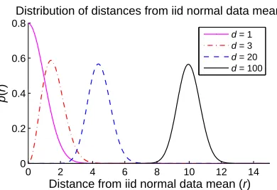
To illustrate the above discussion, Figure 4 depicts, for i.i.d. normal data, the distribution of Euclidean distances of all points to the true data mean (the origin) for several d values. By definition, the distribution of distances is actually the Chi distribution with d degrees of freedom (as the square root of the sum of squares of i.i.d. normal variables, Johnson et al., 1994).8 In this setting, distance concentration refers to the fact that the standard deviation of distance distributions is asymptotically constant with respect to increasing d, while the means of the distance distributions asymptotically behave like √d (a direct consequence of the results by Franc¸ois et al., 2007, discussed further in Section 5.1). On the other hand, for lp-norm distances with p>2, the standard deviation would tend to 0 (Franc¸ois et al., 2007). However, for any finite d, existing variation in the values of random coordinates causes some points to become closer to the distribution mean than others. This happens despite the fact that all distance values, in general, may be increasing together with d.

To understand why points closer to the data mean become hubs in high dimensions, let us consider the following example. We observe, within the i.i.d. normal setting, two points drawn from the data, but at specific positions with respect to the origin: point bd which is at the expected distance from the origin, and point ad which is two standard deviations closer. In light of the above, the distances of adand bdfrom the origin change with increasing d, and it could be said that different ad-s (and bd-s) occupy analogous positions in the data spaces, with respect to changing d. The distances of ad(and bd) to all other points, again following directly from the definition (Oberto and Pennecchi, 2006), are distributed according to noncentral Chi distributions with d degrees of

0 2 4 6 8 10 12 14 0

0.2 0.4 0.6 0.8

Distribution of distances from iid normal data mean

Distance from iid normal data mean (r)

p

(r

)

d = 1 d = 3 d = 20 d = 100

Figure 4: Probability density function of observing a point at distance r from the mean of a multi-variate d-dimensional normal distribution, for d=1,3,20,100.

0 2 4 6 8 10 12 14 16 18

0 0.2 0.4 0.6 0.8

Distance from other points (r)

p

(r

)

Distribution of distances from two points at analogous positions in iid normal data

d = 3 d = 20 d = 100

Dashed line: point at expected dist. from mean Full line: point two standard deviations closer

0 20 40 60 80 100

0.2 0.4 0.6 0.8

d

D

if

fe

re

n

c

e

b

e

tw

e

e

n

m

e

a

n

s

(a) (b)

Figure 5: (a) Distribution of distances to other points from i.i.d. normal random data for a point at the expected distance from the origin (dashed line), and a point two standard deviations closer (full line). (b) Difference between the means of the two distributions, with respect to increasing d.

freedom and noncentrality parameterλequaling the distance of ad (bd) to the origin. Figure 5(a) plots the probability density functions of these distributions for several values of d. It can be seen that, as d increases, the distance distributions for ad and bd move away from each other. This tendency is depicted more clearly in Figure 5(b) which plots the difference between the means of the two distributions with respect to d.

It is known, and expected, for points that are closer to the mean of the data distribution to be closer, on average, to all other points, for any value of d. However, the above analysis indicates that this tendency is amplified by high dimensionality, making points that reside in the proximity of the data mean become closer (in relative terms) to all other points than their low-dimensional analogues are. This tendency causes high-dimensional points that are closer to the mean to have increased inclusion probability into k-NN lists of other points, even for small values of k. We will discuss this relationship further in Section 5.2.

of a point (by increasing its proximity to other points), which, in turn, affects the degree centrality of the corresponding node in the k-NN graph (by increasing its degree, that is, Nk). Other notions of node centrality, and the structure of the k-NN graph in general, will be studied in more detail in Section 5.2.1. The rest of this section will focus on describing the mechanism of the observed spatial centrality amplification.

In the preceding discussion we selected two points from i.i.d. normal data with specific distances from the origin expressed in terms of expected distance and deviation from it, and tracked the analogues of the two points for increasing values of dimensionality d. Generally, we can express the distances of the two points to the origin in terms of “offsets” from the expected distance measured by standard deviation, which in the case of i.i.d. normal random data would be λd,1 =µχ(d)+

c1σ_χ(d)andλd,2=µχ(d)+c2σχ(d), whereλd,1andλd,2are the distances of the first and second point to the origin, µ_χ(d) andσχ(d) are the mean and standard deviation of the Chi distribution with d

degrees of freedom, and c1 and c2 are selected constants (the offsets). In the preceding example involving points ad and bd, we set c1=₋2 and c2=0, respectively. However, analogous behavior can be observed with arbitrary two points whose distance to the data mean is below the expected distance, that is, for c1,c2≤0. We describe this behavior by introducing the following notation:

∆µd(λd,1,λd,2) =|µχ(d,λd,2)−µχ(d,λd,1)|, where µχ(d,λd,i)is the mean of the noncentral Chi distribution

with d degrees of freedom and noncentrality parameterλd,i (i∈ {1,2}). In the following theorem, which we prove in Section 5.1, we show that∆µd(λd,1,λd,2)increases with increasing values of d. Theorem 1 Letλd,1=µχ(d)+c1σχ(d)andλd,2=µχ(d)+c2σχ(d), where d∈N+, c1,c2≤0, c1<c2,

and µ_χ(d) andσ_χ(d)are the mean and standard deviation of the Chi distribution with d degrees of freedom, respectively. Define

∆µd(λd,1,λd,2) =µχ(d,λd,2)−µχ(d,λd,1),

where µ_χ(d,λd,i)is the mean of the noncentral Chi distribution with d degrees of freedom and non-centrality parameterλd,i (i∈ {1,2}).

There exists d0∈Nsuch that for every d>d0,

∆µd(λd,1,λd,2)>0, and

∆µd+2(λd+2,1,λd+2,2)>∆µd(λd,1,λd,2). (1) The main statement of the theorem is given by Equation 1, which expresses the tendency of the difference between the means of the two distance distributions to increase with increasing dimen-sionality d. It is important to note that this tendency is obtained through analysis of distributions of data and distances, implying that the behavior is an inherent property of data distributions in high-dimensional space, rather than an artefact of other factors, such as finite sample size, etc. Through simulation involving randomly generated points we verified the behavior for i.i.d. normal data by replicating very closely the chart shown in Figure 5(b). Furthermore, simulations suggest that the same behavior emerges in i.i.d. uniform data,9 as well as numerous other unimodal random data distributions, producing charts of the same shape as in Figure 5(b). Real data, on the other hand,

tends to be clustered, and can be viewed as originating from a mixture of distributions resulting in a multimodal distribution of data. In this case, the behavior described by Theorem 1, and illustrated in Figure 5(b), is manifested primarily on the individual component distributions of the mixture, that is, on clusters of data points. The next section takes a closer look at the hubness phenomenon in real data sets.

4.3 Hubness in Real Data

Results describing the origins of hubness given in the previous sections were obtained by examining data sets that follow specific distributions and generated as i.i.d. samples from these distributions. To extend these results to real data, we need to take into account two additional factors: (1) real data sets usually contain dependent attributes, and (2) real data sets are usually clustered, that is, points are organized into groups produced by a mixture of distributions instead of originating from a single (unimodal) distribution.

To examine the first factor (dependent attributes), we adopt the approach of Franc¸ois et al. (2007) used in the context of distance concentration. For each data set we randomly permute the elements within every attribute. This way, attributes preserve their individual distributions, but the dependen-cies between them are lost and the intrinsic dimensionality of data sets increases, becoming equal to their embedding dimensionality d (Franc¸ois et al., 2007). In Table 1 (10th column) we give the empirical skewness, denoted as SS_N

k, of the shuffled data. For the vast majority of high-dimensional

data sets, SS_Nk is considerably higher than SNk, indicating that hubness actually depends on the

in-trinsic rather than embedding dimensionality. This provides an explanation for the apparent weaker influence of d on hubness in real data than in synthetic data sets, which was observed in Section 3.2. To examine the second factor (many groups), for every data set we measured: (i) the Spearman correlation, denoted as CN10

dm (12th column), of the observed Nk and distance from the data-set mean, and (ii) the correlation, denoted as CN10

cm (13th column), of the observed Nk and distance to the closest group mean. Groups are determined with K-means clustering, where the number of clusters for each data set, given in column 11 of Table 1, was determined by exhaustive search of values between 2 and_⌊√n_⌋, to maximize CN10

cm.10 In most cases, CcmN10 is considerably stronger than C_dmN10. Consequently, in real data, hubs tend to be closer than other points to their respective cluster centers (which we verified by examining the individual scatter plots).

To further support the above findings, we include the 6th column (dmle) to Table 1, corresponding to intrinsic dimensionality measured by the maximum likelihood estimator (Levina and Bickel, 2005). Next, we compute Spearman correlations between various measurements from Table 1 over all 50 examined data sets, given in Table 2. The observed skewness of Nk, besides being strongly correlated with d, is even more strongly correlated with the intrinsic dimensionality dmle. Moreover, intrinsic dimensionality positively affects the correlations between Nk and the distance to the data-set mean / closest cluster mean, implying that in higher (intrinsic) dimensions the positions of hubs become increasingly localized to the proximity of centers.

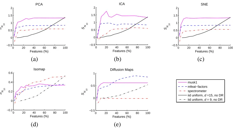
Section 6, which discusses the interaction of hubness with dimensionality reduction, will pro-vide even more support to the observation that hubness depends on intrinsic, rather than embedding dimensionality.

10. We report averages of CN10

cm over 10 runs of K-means clustering with different random seeding, in order to reduce the

d dmle SN10 C

N10

dm C

N10

cm BNf10 CNBN1010

dmle 0.87

SN10 0.62 0.80

CN10

dm −0.52−0.60−0.42

CN10

cm −0.43−0.48−0.31 0.82

f

BN10 −0.05 0.03−0.08−0.32−0.18

CN10

BN10 0.32 0.39 0.29−0.61−0.46 0.82 CAV 0.03 0.03 0.03−0.14−0.05 0.85 0.76

Table 2: Spearman correlations over 50 real data sets.

0 2 4 6 8 10 12 0

20 40 60

Distance from k−th NN

Nk

ionosphere

4 6 8 10 12 14 16 0

20 40 60

Distance from k−th NN

N k

sonar

(a) (b)

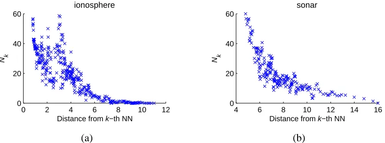
Figure 6: Correlation between low Nkand outlier score (k=20).

4.4 Hubs and Outliers

The non-negligible variance of the distribution of distances to the data mean described in Sec-tion 4.2 has an addiSec-tional “side”: we also expect points farther from the mean and, therefore, with much lower observed Nk than the rest.11 Such points correspond to the bottom-right parts of Fig-ure 3(b, c, e, f), and will be referred to as antihubs. Since antihubs are far away from all other points, in high dimensions they can be regarded as distance-based outliers (Tan et al., 2005).

To further support the connection between antihubs and distance-based outliers, let us consider a common outlier score of a point as the distance from its kth nearest neighbor (Tan et al., 2005). Low Nkvalues and high outlier scores are correlated as exemplified in Figure 6(a, b) (in their lower-right parts) for two data sets from Table 1.

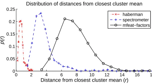
Next, let us recall the i.i.d. normal random data setting, and the probability density function corresponding to observing a point at a specified distance from the mean, plotted in Figure 4. An analogous chart for real data is given in Figure 7, which shows the empirical distributions of dis-tances from the closest cluster mean for three real data sets, as described in Section 4.3. In both figures it can be seen that in low dimensions the probability of observing a point near a center is quite high, while as dimensionality increases it becomes close to zero. If we now consider a probabilistic definition of an outlier as a point with a low probability of occurrence (Tan et al., 2005), in high

11. Assuming the presence of hubs, the existence of points with low Nkis implied by the constant-sum property of Nk:

0 2 4 6 8 10 12 14 16 18 0

0.05 0.1 0.15 0.2 0.25

Distribution of distances from closest cluster mean

Distance from closest cluster mean (r)

p

(r

)

haberman spectrometer mfeat−factors

Figure 7: Probability density function of observing a point at distance r from the closest cluster mean for three real data sets.

dimensions hubs actually are outliers, as points closer to the distribution (or cluster) mean than the majority of other points. Therefore, somewhat counterintuitively, it can be said that hubs are points that reside in low-density regions of the high-dimensional data space, and are at the same time close to many other points. On the other hand, distance-based outliers correspond to probabilistic out-liers that are farther away from the center(s). It follows that the definitions of distance-based and probabilistic outliers significantly diverge from one another in high dimensions, with distance-based outliers only partially corresponding to probabilistic outliers. To prevent confusion in the rest of the paper, we shall continue to refer to “hubs” and “outliers” in the distance-based sense. Outliers will be analyzed further in Section 7.3.2.

5. Proofs and Discussion

This section is predominantly devoted to the theoretical aspects of the behavior of distances in high-dimensional space and the hubness phenomenon. Section 5.1 provides a step-by-step proof of Theorem 1 which was introduced in Section 4.2, while Section 5.2 discusses additional aspects of the phenomenon in the context of the geometry of high-dimensional spaces and the properties of data distributions which occupy them.

5.1 Proof of Theorem 1

5.1.1 DISTANCECONCENTRATIONRESULTS

We begin by reviewing the main results of Franc¸ois et al. (2007) regarding distance concentration. Let Xd= (X1,X2, . . . ,Xd)be a random d-dimensional variable with i.i.d. components: Xi_∼

F

|F_|2 signify their

mean and variance, respectively. Franc¸ois et al. (2007) prove the following two lemmas.12 Lemma 2 (Franc¸ois et al., 2007, Equation 17, adapted)

lim d→∞

E(_kXd_k)

√

d =µ|F|2.

Lemma 3 (Franc¸ois et al., 2007, Equation 21, adapted)

lim

d_→∞Var(kXdk) =

σ2

|F_|2

4µ_|F_|2

.

The above lemmas imply that, for i.i.d. random data, the expectation of the distribution of Eu-clidean distances to the origin (EuEu-clidean norms) asymptotically behaves like√d, while the stan-dard deviation is asymptotically constant. From now on, we will denote the mean and variance of random variables that are distributed according to some distribution

F

5.1.2 DISTANCES IN I.I.D. NORMALDATA

We now observe more closely the behavior of distances in i.i.d. normal random data. Let Zd = (Z1,Z2, . . . ,Zd) be a random d-dimensional vector whose components independently follow the standard normal distribution: Zi∼

N

χ(d)is the distribution of Euclidean distances of vectors drawn from Zd to the origin. If one were to fix another reference vector xdinstead of the origin, the distribution of distances of vectors drawn from Zdto xdwould be completely determined bykxdksince, again by definition, random variable

kZd₋xd_k follows the noncentral Chi distribution with d degrees of freedom and noncentrality parameterλ=_kxdk:kZd−xdk ∼χ(d,kxdk).

In light of the above, let us observe two points, xd,1and xd,2, drawn from Zd, and express their

distances from the origin in terms of offsets from the expected distance, with the offsets described using standard deviations: _kxd,1k=µχ(d)+c1σχ(d)andkxd,2k=µχ(d)+c2σχ(d), where c1,c2≤0. We will assume c1<c2, that is, xd,1is closer to the data distribution mean (the origin) than xd,2. By treating c1and c2as constants, and varying d, we observe analogues of two points in spaces of dif-ferent dimensionalities (roughly speaking, points xd,1 have identical “probability” of occurrence at the specified distance from the origin for every d, and the same holds for xd,2). Letλd,1=kxd,1k andλd,2=kxd,2k. Then, the distributions of distances of points xd,1and xd,2to all points from the data distribution Zd (that is, the distributions of random variableskZd−xd,1kandkZd−xd,2k) are noncentral Chi distributionsχ(d,λd,1)andχ(d,λd,2), respectively. We study the behavior of these two distributions with increasing values of d.

behave like√d as d→∞, whileσ2_χ(d,λ

d,1)andσ

2

χ(d,λd,2)are both asymptotically constant.

13 _However, for xd,1 and xd,2 placed at different distances form the origin (λd,16=λd,2, that is, c16=c2), these

asymptotic tendencies do not occur at the same speed. In particular, we will show that as d increases, the difference between µ_χ(d,λd,1)and µχ(d,λd,2)actually increases. If we take xd,1to be closer to the

origin than xd,2 (c1 <c2), this means that xd,1 becomes closer to all other points from the data distribution Zd than xd,2, simply by virtue of increasing dimensionality, since for different values

of d we place the two points at analogous positions in the data space with regards to the distance from the origin.

5.1.3 ASYMPTOTICEQUIVALENCE

Before describing our main theoretical result, we present several definitions and lemmas, beginning with the notion of asymptotic equivalence that will be relied upon.

Definition 4 Two real-valued functions f(x)and g(x)are asymptotically equal, f(x)_≈g(x), iff for everyε>0 there exists x0_∈R_{such that for every x>x0,|f(x)−g(x)|<}ε_.

Equivalently, f(x)_≈g(x)iff limx_→∞|f(x)₋g(x)_|=0. Note that the_≈relation is different from the divisive notion of asymptotic equivalence, where f(x)_∼g(x)iff limx_→∞f(x)/g(x) =1.

The following two lemmas describe approximations that will be used in the proof of Theorem 1, based on the_≈relation.

Lemma 5 For any constant c_∈R_{, let f(d) =}√_{d+c,and g(d) =}√_{d.Then, f(d)≈g(d).}

Proof

lim d→∞

√d+c₋√d

= lim

d→∞ _√

d+c₋√d

√

d+c+√d

√

d+c+√d

=dlim→∞

c √

d+c+√d

=0.

Lemma 6 µ_χ(d)≈ √

d, andσ_χ(d)≈1/ √

2.

Proof Observe the expression for the mean of theχ(d)distribution,

µ_χ(d)= √

2Γ d+1

2

Γ d 2

.

The equality xΓ(x) =Γ(x+1)and the convexity of logΓ(x)yield (Haagerup, 1982, p. 237):

Γd+1

2 2 ≤Γ d 2

Γd+2

2 =d 2Γ d 2 2 ,

13. More precisely, the lemmas can be applied only for points x′_d,i that have equal values of all components, since after translation data components need to be i.i.d. Because of the symmetry of the Gaussian distribution, the same expectations and variances of distance distributions are obtained, for every d, with any xd,ithat has the same norm as

and

Γd+1

2

2

=d−1

2 Γ

d₋1

2

Γd+1

2

≥d−₂1Γ

d 2

2 ,

from which we have

√

d₋1_≤√2Γ

d+1 2

Γ d 2

≤√d.

From Lemma 5 it now follows that µ_χ(d)≈√d .

Regarding the standard deviation of the χ(d)distribution, from Lemma 3, taking

F

lim d→∞σ

2 χ(d)=

σ2 χ2₍₁₎

4µ_χ2₍₁₎

= 1

2,

since the square of a standard normal random variable follows the chi-square distribution with one degree of freedom,χ2(1), whose mean and variance are known: µ_χ2₍₁₎=1, σ2_χ2

(1)=2. It now

di-rectly follows thatσ_χ(d)≈1/ √

2.

5.1.4 EXPECTATION OF THENONCENTRALCHIDISTRIBUTION

The central notion in Theorem 1 is the noncentral Chi distribution. To express the expectation of the noncentral Chi distribution, the following two definitions are needed, introducing the Kummer confluent hypergeometric function1F1, and the generalized Laguerre function.

Definition 7 (Itˆo, 1993, p. 1799, Appendix A, Table 19.I)

For a,b,z_∈R_{, the Kummer confluent hypergeometric function1F1(a; b; z)is given by}

1F1(a; b; z) = ∞

∑

k=0

(a)k

(b)k · zk

Γ(k+1),

where(_·)kis the Pochhammer symbol,(x)k= Γ(_Γx₍+_x)k).

Definition 8 (Itˆo, 1993, p. 1811, Appendix A, Table 20.VI)

Forν,α,z_∈R_{, the generalized Laguerre function L}(_να)_{(z)is given by}

L(_να)(z) =Γ(ν+α+1)

Γ(ν+1) ·

1F1(−ν;α+1; z)

Γ(α+1) .

The expectation of the noncentral Chi distribution with d degrees of freedom and noncentrality parameterλ, denoted by µ_χ(d,λ), can now be expressed via the generalized Laguerre function (Oberto

and Pennecchi, 2006):

µ_χ(d,λ)= r_π

2L

(d/2−1)

1/2

−λ

2 2

5.1.5 PROPERTIES OF THE GENERALIZEDLAGUERREFUNCTION

The proof of Theorem 1 will rely on several properties of the generalized Laguerre function. In this section we will review two known properties and prove several additional ones as lemmas.

An important property of the generalized Laguerre function is its infinite differentiability in z, with the result of differentiation again being a generalized Laguerre function:

∂ ∂zL

(α)

ν (z) =₋L(_να₋+₁1)(z). (3) Another useful property is the following recurrence relation:

L(_να)(z) =L_ν(α₋)₁(z) +L(_να−1)(z). (4)

Lemma 9 Forα>0 and z<0:

(a) L(₋α₁)_/2(z)is a positive monotonically increasing function in z, while (b) L(₁α_/2)(z)is a positive monotonically decreasing concave function in z. Proof (a) From Definition 8,

L(₋α₁)_/2(z) =Γ(α+1/2)

Γ(1/2) ·

1F1(1/2;α+1; z)

Γ(α+1) .

Sinceα>0 all three terms involving the Gamma function are positive. We transform the remaining term using the equality (Itˆo, 1993, p. 1799, Appendix A, Table 19.I):

1F1(a; b; z) =ez1F1(b−a; b;−z), (5)

which holds arbitrary a,b,z_∈R_{, obtaining}

1F1(1/2;α+1; z) =ez1F1(α+1/2;α+1;−z).

From Definition 7 it now directly follows that L(₋α₁)_/2(z)is positive forα>0 and z<0.

To show that L(₋α₁)_/2(z) is monotonically increasing in z, from Equation 3 and Definition 8 we have

∂ ∂zL

(α)

−1/2(z) =−L

(α+1)

−3/2 (z) =−

Γ(α+1/2)

Γ(₋1/2) ·

1F1(3/2;α+2; z)

Γ(α+2) .

Forα>0 and z<0, from Equation 5 it follows that1F1(3/2;α+2; z)>0. SinceΓ(₋1/2)<0 and all remaining terms are positive, it follows that₋L(₋α₃+_/21)(z)>0. Thus, L(₋α₁)_/2(z)is monotonically increasing in z.

(b) Proofs that L(₁α_/2)(z)is positive and monotonically decreasing are very similar to the proofs in part (a), and will be omitted. To address concavity, we observe the second derivative of L(₁α_/)₂(z):

∂2

∂zL

(α)

1/2(z) =L

(α+2) −3/2(z) =

Γ(α+3/2)

Γ(₋1/2) ·

1F1(3/2;α+3; z)

Γ(α+3) .

Lemma 10 Forα>0 and z<0, L(₁α_/+₂1)(z)_≈L(₁α_/)₂(z). Proof From the recurrence relation in Equation 4 we obtain

L(₁α_/+₂1)(z) =L₋(α₁+_/1₂)(z) +L(₁α_/)₂(z). Therefore, to prove the lemma it needs to be shown that for z<0,

lim α→∞L

(α)

−1/2(z) =0. (6)

From Definition 8 and Equation 5 we have

L(₋α₁)_/2(z) = e−

z

Γ(1/2)·

Γ(α+1/2)

Γ(α+1) ·1F1(α+1/2;α+1;−z).

From the asymptotic expansion by Fujikoshi (2007, p. 16, adapted),

1F1

1 2n;

1

2(n+b); x

=ex 1+O(n−1), (7)

where n is large and x_≥0, it follows that lim_α→∞1F1(α+1/2;α+1;−z)<∞.Thus, to prove Equation 6 and the lemma it remains to be shown that

lim α→∞

Γ(α+1/2)

Γ(α+1) =0. (8)

As in the proof of Lemma 6, from the inequalities derived by Haagerup (1982) we have

p

β₋1_≤√2

Γβ+1 2

Γβ₂ ≤ p

β,

whereβ>1. Applying inversion and substitutingβwith 2α+1 yields the desired limit.

Lemma 11 Forα>1/2 and z<0: (a) limz_→−∞L(₋α₃)_/2(z) =0, and (b) limα→∞L(₋α3)/2(z) =0.

Proof (a) From Definition 8 we have

L(₋α₃)_/2(z) =Γ(α−1/2)

Γ(₋1/2) ·

1F1(3/2;α+1; z)

Γ(α+1) . (9)

The following property (Abramowitz and Stegun, 1964, p. 504, Equation 13.1.5),

1F1(a; b; z) = Γ

(b)

Γ(b₋a)(−z)

a _1+O(

when substituted into Equation 9, taking a=3/2 and b=α+1, yields

L(₋α₃)_/2(z) = 1

Γ(₋1/2)(−z)−

3/2 _1+O(|z|−1_{). (10)} From Equation 10 the desired limit directly follows.

(b) The proof of part (b) is analogous to the proof of Lemma 10, that is, Equation 6. From Definition 8 and Equation 5, after applying the expansion by Fujikoshi (2007) given in Equation 7, it remains to be shown that

lim α→∞

Γ(α₋1/2)

Γ(α+1) =0. (11)

SinceΓ(α₋1/2)<Γ(α+1/2)for everyα≥2, the desired limit in Equation 11 follows directly from Equation 8.

5.1.6 THEMAINRESULT

This section restates and proves our main theoretical result.

Theorem 1 Letλd,1=µχ(d)+c1σχ(d)andλd,2=µχ(d)+c2σχ(d), where d∈N+, c1,c2≤0, c1<c2, and µ_χ(d) andσχ(d)are the mean and standard deviation of the Chi distribution with d degrees of

freedom, respectively. Define

∆µd(λd,1,λd,2) =µχ(d,λd,2)−µχ(d,λd,1),

where µ_χ(d,λd,i)is the mean of the noncentral Chi distribution with d degrees of freedom and

non-centrality parameterλd,i (i∈ {1,2}).

There exists d0∈Nsuch that for every d>d0,

∆µd(λd,1,λd,2)>0, (12)

and

∆µd+2(λd+2,1,λd+2,2)>∆µd(λd,1,λd,2). (13) Proof To prove Equation 12, we observe that for d>2,

∆µd(λd,1,λd,2) = µχ(d,λd,2)−µχ(d,λd,1)

=

r_π

2 L

(d 2−1)

1/2 −

λ2 d,2 2

! −

r_π

2 L

(d 2−1)

1/2 −

λ2 d,1 2

!

> 0,

where the last inequality holds for d>2 because λd,1<λd,2, and L₁(d_//₂2−1)(z) is a monotonically decreasing function in z<0 for d/2₋1>0 (Lemma 9).

In order to prove Equation 13, we will use approximate values of noncentrality parametersλd,1 andλd,2. Letbλd,1=

√

d+c1/

√

2, andbλd,2=

√

d+c2/

√

2. From Lemma 6 it follows thatbλd,1≈λd,1 andbλd,2≈λd,2. Thus, by proving that there exists d2∈Nsuch that for every d>d2,

we prove that there exists d1∈N_{such that for every d>d1 Equation 13 holds. The existence of} such d1, when approximations are used as function arguments, is ensured by the fact that L(₁α_/)₂(z)is a monotonically decreasing concave function in z (Lemma 9), and by the transition fromαtoα+1 having an insignificant impact on the value of the Laguerre function for large enoughα(Lemma 10). Once Equation 14 is proven, Equations 12 and 13 will hold for every d>d0, where d0=max(2,d1).

To prove Equation 14, from Equation 2 it follows we need to show that

L(₁d_//₂2)

−1₂√d+2+c2/√22

−L(₁d_//₂2)

−1₂√d+2+c1/√22

> L(₁d_//₂2−1)

−1₂√d+c2/

√

22

−L(₁d_//₂2−1)

−1₂√d+c1/

√

22

. (15)

We observe the second derivative of L(₁α_/)₂(z):

∂2

∂zL

(α)

1/2(z) =L

(α+2) −3/2 (z).

Since L(₋α₃+_/2₂)(z)tends to 0 as z→ −∞, and tends to 0 also asα→∞(Lemma 11), it follows that the two Laguerre functions on the left side of Equation 15 can be approximated by a linear function with an arbitrary degree of accuracy for large enough d. More precisely, since L(₁α_/)₂(z)is monotonically decreasing in z (Lemma 9) there exist a,b_∈R_{, a>0, such that the left side of Equation 15, for} large enough d, can be replaced by

−a

−1

2

_√

d+2+c2/√2

2

+b −

−a −1 2 _√

d+2+c1/√2

2 +b = a 2 _√

d+2+c2/

√

22₋a 2

_√

d+2+c1/

√

22. (16)

From Lemma 10 it follows that the same linear approximation can be used for the right side of Equation 15, replacing it by

a 2

_√

d+c2/√22₋a 2

_√

d+c1/√22. (17)

After substituting the left and right side of Equation 15 with Equations 16 and 17, respectively, it remains to be shown that

a 2

_√

d+2+c2/

√

22₋a 2

_√

d+2+c1/

√

22 >a

2

_√

d+c2/

√

22₋a 2

_√

d+c1/

√

22. (18)

Multiplying both sides by√2/a, moving the right side to the left, and applying algebraic simplifi-cation reduces Equation 18 to

c2−c1

_√

d+2₋√d>0,

5.2 Discussion

This section will discuss several additional considerations and related work regarding the geometry of high-dimensional spaces and the behavior of data distributions within them. First, let us consider the geometric upper limit to the number of points that point x can be a nearest neighbor of, in Euclidean space. In one dimension, this number is 2, in two dimensions it is 5, while in 3 dimensions it equals 11 (Tversky and Hutchinson, 1986). Generally, for Euclidean space of dimensionality d this number is equal to the kissing number, which is the maximal number of hyperspheres that can be placed to touch a given hypersphere without overlapping, with all hyperspheres being of the same size.14 Exact kissing numbers for arbitrary d are generally not known, however there exist bounds which imply that they progress exponentially with d (Odlyzko and Sloane, 1979; Zeger and Gersho, 1994). Furthermore, when considering k nearest neighbors for k>1, the bounds become even larger. Therefore, only for very low values of d geometrical constraints of vector space prevent hubness. On the other hand, for higher values of d hubness may or may not occur, and the geometric bounds, besides providing “room” for hubness (even for values of k as low as 1) do not contribute much in fully characterizing the hubness phenomenon. Therefore, in high dimensions the behavior of data distributions needed to be studied.

We focus the rest of the discussion around the following important result,15 drawing parallels with our results and analysis, and extending existing interpretations.

Theorem 12 (Newman and Rinott, 1985, p. 803, Theorem 3, adapted)

Let x(i)= (x(₁i), . . . ,x_d(i)), i=0, . . . ,n be a sample of n+1 i.i.d. points from distribution F(X), X= (X1, . . . ,Xd)_∈Rd_{. Assume that F is of the form F(X) =}∏d_k=1

F

k=1g(x

(i)

k ,x

(j)

k ). Let N n,d 1 denote the number of points among_{x(1), . . . ,x(n)_}whose nearest neighbor is x(0).

Suppose 0<Var(g(X,Y))<∞and set

β=Correlation(g(X,Y),g(X,Z)), (19)

where X,Y,Z are i.i.d. with common distribution

F

lim n→∞dlim→∞N

n,d

1 =Poisson(λ=1) in distribution (20) and

lim

n→∞dlim→∞Var(N

n,d

1 ) =1. (21)

(b) Ifβ>0 then

lim n→∞dlim→∞N

n,d

1 =0 in distribution (22)

while

lim

n→∞dlim→∞Var(N

n,d

1 ) =∞. (23)

14. If ties are disallowed, it may be necessary to subtract 1 from the kissing number to obtain the maximum of N1.