in the population sciences published by the Max Planck Institute for Demographic Research Konrad-Zuse Str. 1, D-18057 Rostock · GERMANY www.demographic-research.org
DEMOGRAPHIC RESEARCH
VOLUME 14, ARTICLE 11, PAGES 217-236
PUBLISHED 16 MARCH 2006
http://www.demographic-research.org/Volumes/Vol14/11/ DOI: 10.4054/DemRes.2006.14.11
Research Article
Ages of origin and destination for a difference in
life expectancy
Elwood Carlson
2 Ages where a difference in life expectancy originates 220
3 Destination ages where a difference in life expectancy is lived 223
4 Bridging between origin and destination decomposition 226
References 231
Ages of origin and destination for a difference in life expectancy
Elwood Carlson 1
Abstract
Decomposition of a difference in life expectancies may identify ages at which the difference originates in mortality differences, or may identify ages at which the difference results in different values of person-years lived (life table population). This study shows that the two approaches are orthogonally related to each other, and derives an origin-destination decomposition matrix in which summing in one direction produces Andreev's origin-decomposition results, while summing in the other direction produces destination-decomposition corresponding to directly-observed differences in nLx values.
1. Salience of the life expectancy measure
The life table provides a convenient, comprehensive and self-contained summary of mortality conditions prevailing in an actual or hypothetical population. The relations among its columns and parameters have formed one of the most fruitful traditions of mathematical population research.
Of all the summary measures that can be derived from a life table, the expectation of life (or life expectancy) is perhaps the most well-known, widely-used, widely-cited and widely-studied statistic. For any age x (most frequently, age zero or birth) ex reports the mean number of person-years each person attaining age x can expect to live, given the mortality rates observed throughout the entire life table. Two different life tables, reflecting conditions in two different populations or in a single population at two different times, ordinarily report two different expectations of life at any age.
Briefly, this expectation of life at any age depends on two life table measures, survivors to exact age lx and total person-years lived nLi in age groups above age x. Both measures derive from observed risks of death in each age group (Chiang 1984, Preston et al 2001). The expectation of life at any age x simply divides the person-years left to live above age x by the number of survivors to that age who are left to live them:
. ,
x n x i
i n
x
l L e
∑
Ω=
= (1)
To simplify our descriptions, we introduce some standard extensions of basic life table notation. A bar over lx or ex indicates the arithmetic mean of lx or ex values from different life tables, as defined by equation 2:
. 2 ; 2 + = +
= bx
a x x b x a x x e e e l l
l (2)
As defined by Arriaga (1984), the nex measure of temporary life expectancy represents person-years lived within a specific age interval, per person alive at the start of the interval (dividing nLx by lx as in equation 3 below). It also can represent the ratio of the probability of dying in the interval to the average force of mortality during the interval (dividing nqx by nmx as in equation 3).
. x n x n x x n x n m q l L
e = = (3)
We also define an extension of temporary life expectancy, called conditional temporary life expectancy, as person-years lived in some age interval above the age group x to x+n, per person alive at exact age x, the "baseline age" for this partial measure. Conditional temporary life expectancy can be written:
.
,i x
l L e x i n x i
n = ≥ (4)
Since all conditional temporary life expectancies starting at the same baseline age share the same denominator lx, the sum of all these terms (including the unconditional or "ordinary" temporary life expectancy, when i equals x) is simply the expectation of life at age x as shown in equation 5 below.
2. Ages where a difference in life expectancy originates
Several popular decompositions of a difference in life expectancy ask about the origin of the difference. That is, they allocate a difference across ages where mortality differences first influence the number of person-years to be lived at subsequent ages (Shkolnikov, Valkonen, Begun & Andreev, 2001). This origin-decomposition approach includes the well-known methods of Arriaga (1984), Andreev (1982) and Pressat (1982). An origin-decomposition breaks down a difference in life expectancy at birth according to the ages at which the lives are originally saved (but see Vaupel & Yashin 1987 on the thorny issue of “repeated lifesaving”). For simplicity we consider the origin-decomposition proposed by Andreev (1982), who calculated two versions of an age-specific measure n
ε
x and then averaged the two:[
( )] [
( b )]
, n x a n x a n x b x a x a x a xnε = l ⋅ e −e − l + ⋅ e+ −e+ (6a)
[
( )] [
( xa n)]
, b n x b n x a x b x b x b xnε = l ⋅ e −e −l + ⋅ e+ −e+ (6b)
( )
. 2 , 0 , 0 00
∑
∑
Ω = Ω = − = = − n x a x n b x n n x x n a b e
e ε ε ε (6c)
The average in the final term of equation 6c subtracts rather than adds because the reversed order of subtraction of life expectancies in 6a and 6b give the two partial terms opposite signs. Taking the average of lx values (see equation 2 above) from the outset seems simpler, as shown in equation 7 below, which yields identical results:
( )
(
[
(
)
]
[
(
)
]
)
. , 0 , 0 00
∑
∑
Ω = + + + Ω = − ⋅ − − ⋅ = = − n x a n x b n x n x a x b x x n x x n a b e e l e e l e
e ε (7)
For each age group, one finds the weighted difference in person-years lived above age x (the first term) and then subtracts the weighted difference lived above age x+n (the second term) to attribute n
ε
x to the age group itself as a remainder. The weights are simply averages of the lx values in the populations. For the last open-ended interval in a life table, the second term in equation 7 equals zero because ex+n does not exist.To illustrate this origin-decomposition of differences in life expectancy at birth, consider life table values for the black and white male and female populations of the United States in the year 2000 as shown in Table 1.
Table 1: Survival values by race and sex, United States 2000
Black Black White White Black Black White White
Male Female Male Female Male Female Male Female
Age x lx lx lx lx nLx nLx nLx nLx
0 1,000000 1,000000 1,000000 1,000000 0,986323 0,988863 0,994520 0,995500
1 0,984440 0,987330 0,993760 0,994870 3,931890 3,944600 3,971985 3,977035
5 0,982060 0,985350 0,992470 0,993860 4,906625 4,925205 4,960130 4,967590
10 0,980710 0,984300 0,991630 0,993200 4,900490 4,919035 4,956065 4,964405
15 0,979050 0,983210 0,990460 0,992430 4,881350 4,911105 4,942410 4,957535
20 0,972590 0,981000 0,986040 0,990460 4,835370 4,896300 4,914825 4,946955
25 0,961070 0,977300 0,979770 0,988310 4,774945 4,874740 4,883480 4,935595
30 0,948860 0,972320 0,973630 0,985860 4,711295 4,844540 4,851580 4,921870
35 0,935310 0,965060 0,966750 0,982680 4,636110 4,800870 4,811970 4,901955
40 0,918270 0,954620 0,957550 0,977770 4,533170 4,736175 4,756930 4,871595
45 0,893330 0,938790 0,944410 0,970440 4,376095 4,637950 4,675745 4,827210
50 0,854640 0,915090 0,924740 0,959700 4,143885 4,499440 4,559055 4,759335
55 0,800330 0,883290 0,897310 0,942830 3,830325 4,315295 4,389845 4,651825
60 0,728840 0,840460 0,855860 0,915900 3,428780 4,058430 4,134605 4,481505
65 0,640480 0,779960 0,794190 0,873850 2,959500 3,710160 3,763960 4,233190
70 0,540820 0,700400 0,706570 0,811630 2,411275 3,245505 3,249725 3,848085
75 0,421010 0,593330 0,588740 0,722540 1,784990 2,646445 2,593935 3,316440
80 0,293170 0,462100 0,445210 0,597920 1,160305 1,946530 1,819305 2,589670
85 0,173540 0,314100 0,281000 0,431120 0,624270 1,202460 1,019395 1,685395
90 0,082120 0,171120 0,133350 0,244390 0,263825 0,579340 0,412640 0,825485
95 0,029410 0,068920 0,042170 0,096380 0,083085 0,199285 0,107340 0,267860
100 0,007540 0,018310 0,007730 0,022440 0,021720 0,049360 0,017030 0,053510
68,185623 74,931633 74,786475 79,979545
Table 1 shows proportions of each race/sex group surviving to specified ages, and also the person-years lived in each age interval including the final open-ended interval. As suggested by equation 1 above, the sum at the bottom of each nLx column gives the expectation of life at birth. Black males had the lowest life expectancy at birth in 2000. Differences in e0 by race and sex were roughly equal in size and additive. That is, both black females and white males could expect about six more years of life based on 2000 mortality rates than could black males. White females had the highest expectation of life.
Andreev's n
ε
x age decomposition allocates differences in life expectancy according to the age group where the mortality difference first occurs, so we classify this approach as an origin-decomposition. It aims to identify the age groups where changes in life expectancy originate. Figure 1 concentrates attention on black men because their survival rates were worst in 2000, showing a sex difference on one hand (black men compared to black women) and a race difference on the other (black men compared to white men).Figure 1: Age origin of Black male deficit in life expectancy by race or sex
-0.1 0.0 0.1 0.2 0.3 0.4 0.5 0.6 0.7 0.8 0.9
0 1 5 10 15 20 25 30 35 40 45 50 55 60 65 70 75 80 85 90 95 100
Yea
rs
o
f L
ife
Sex Race
Compared to white men, black men in the United States in 2000 experienced much higher rates of infant death, accounting for over one-tenth of the total difference in life expectancy at birth. On the other hand, higher death rates for black than for white boys between ages 1 and 15 had very little impact on the difference in expectation of life, in part because the rates themselves were so low at these ages for both groups, and in part because the difference in death rates by race was relatively small. Age-specific contributions to the race difference in life expectancy for American men in 2000 increased gradually after childhood, however, and peaked in the late working ages (roughly 45 to 65) where almost half of the total difference in life expectancy at birth originated. Older ages contribute much less to the race difference in life expectancy, in part because there are fewer survivors left at these older ages to contribute person-years lived, and in part because reported mortality rates converge in old age for black and white men. This convergence has been the subject of intense interest, and its significance continues to be debated.
Compared to black women, black men in the United States in 2000 exhibited a life expectancy disadvantage that very closely resembled the race contrast between black and white men in both absolute magnitude (6.75 years for the sex contrast versus 6.60 years for the race contrast) and in its ages of origin. The major differences between the two age patterns in Figure 1 are that infancy contributed much less to the sex contrast while young adulthood (when males of all backgrounds seem to exhibit anomalously high mortality rates) contributed more to the sex contrast. Mortality differences originating in late middle age and early retirement dominate both age and sex contrasts. At these ages most people are still alive but a lifetime of various social, economic and health effects begin to take their cumulative toll and death rates rise prematurely for disadvantaged groups. The sex difference in life expectancy also owes more to mortality differences in old age than does the race difference.
3. Destination ages where a difference in life expectancy is lived
For conventional period life table analysis, origin-decomposition often proves most useful because such life tables represent fictional extrapolations from actual mortality conditions to a synthetic "life table population" that only exists conceptually. Naturally, we most commonly wish to understand how these actual conditions affect the resulting thought-experiment that is the life table.
difference in mortality by sex affects the sex ratio in different age groups may interest family scholars. In the case of cohort life tables that follow actual generations over time, the destinations at which person-years are lived also correspond to real-world circumstances, so that destination-decomposition may be of intrinsic interest. Similarly, simulation exercises such as experiments with stable population theory (where all features of the life table may be hypothetical) also may find the destination ages where a difference in life expectancy is lived to be of equal importance with the origin ages where mortality differences give rise to such effects.
In its simplest form, destination-decomposition operates directly on nLx values, taking advantage of the fact that by re-arranging equation 3 above, each nLx can be expressed as the product of survivors to the start of the age group lx and the temporary life expectancy nex. Use of a new age subscript i emphasizes the distinction between ages of origin and ages of destination as alternate decompositions. With two terms, we may consider ordinary component decomposition (Das Gupta 1978, 1994). Equation 8 below includes two components.
(
)
(
( )) (
( ))
., 0 ,
0 0
0
∑
∑
Ω
= Ω
=
− ⋅ + − ⋅ = − =
−
n i
a i b i i n a i n b i n i n
i
a i n b i n a
b e L L l e e e l l
e (8)
Figure 2: Destination ages for Black male deficit in life expectancy by race or sex
-0.1 0.0 0.1 0.2 0.3 0.4 0.5 0.6 0.7 0.8 0.9 1.0
0 1 5 10 15 20 25 30 35 40 45 50 55 60 65 70 75 80 85 90 95 100
Ye
a
rs
o
f L
if
e
Sex Race Source: data in Table 1.
Using the same data from Table 1 to compute the destination-decomposition of differences in nLi values directly, Figure 2 displays a completely different way of thinking about a decomposition of a difference in life expectancy in contrast to Figure 1. The two alternative decompositions represent answers to different questions. An origin-decomposition tells us at which ages a difference in life expectancy originates. A destination-decomposition tells us at which ages a difference in life expectancy is lived. Both decompositions add up to the total difference in life expectancy, but Figure 2 attributes much less of the difference to young ages where differences in person-years lived within the age groups were quite small, and places greater emphasis on older ages at which differences in death rates from earlier ages result in new person-years of life.
person-years lived in each age group nLx. In proper dialectic form, the final section of this analysis provides the synthesis that connects the two.
4. Bridging between origin and destination decomposition
We may expand an origin-decomposition such as Andreev’s into a series of terms involving temporary and conditional temporary life expectancy as described above. When we do this, the first bracketed term from equation 7 becomes a difference in temporary life expectancy nex weighted by the averaged lx value (a “direct” effect), plus a series of differences in conditional temporary life expectancies for older age groups also weighted by the averaged lx value (the second bracketed term in equation 9a below). The direct effect (the first bracketed term in equation 9a) closely resembles the direct effect specified by Arriaga (1984) except that Arriaga’s method did not average the lx values, privileging one of them as a baseline. Note that this direct effect is identical to the direct effect specified in equation 8 above for destination-decomposition.
( )
(
)
[
]
(
)
(
)
.0 , ,
0 0
∑
∑
∑
∑
Ω = Ω + = + + + Ω + = ⋅ − − ⋅ − + − ⋅ = = = −x i xnn
a n x i n b n x i n n x n n x i a x i n b x i n x a x n b x n x x x n a b e e l e e l e e l e e ε (9a)
The second bracketed term from equation 7, when expanded in terms of conditional temporary life expectancy as shown in the third bracketed term of equation 9a above, contains no reference to the age group from x to x+n. However, it does contain a series of expressions for older age groups that match one-for-one with the equation's second bracketed term. The third term differs from the second term in that the baseline age becomes x+n rather than x. Since the two summations cover the same ages, we may re-arrange the second and third terms as shown in equation 9b below:
( )
(
)
(
)
[
(
(
)
)
(
(
)
)
]
. 0 , 0 0∑
∑
∑
Ω = Ω + = + + + ⋅ − + ⋅ − − ⋅ − = = = −x i x nn
Andreev's n
ε
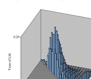
x expression for a difference in life expectancy originating in a given age group thus breaks down across all subsequent age groups using the terms in equation 9b above. We can see not only how much of the total difference in life expectancy originated in each age group, but also in which age groups that portion of the total difference subsequently was lived.For example, consider the n
ε
x age decomposition of the race difference in life expectancy between black men and white men in the United States in 2000, depicted in Figure 1 above. Appendix Table A distributes each difference originating in a specific age group across subsequent age groups where that difference would be lived out in the life table. The first cell with a value for each age group (row of Appendix Table A) shows the direct effect as the average of lx values times the difference in nex values. Subsequent cells in that row contain the sequence of differenced, weighted nei|x differences as described in equation 9b. Each step of the summation over i yields a value for another age group in the row. Together, the values in each row sum to Andreev's nε
x effect. Summing over x then produces the total difference in life expectancy.Figure 3: Origin & destination of race difference in life expectancy (U.S. White men-Black men)
0 10 25 40 55 70 85 100
0 20
45 70
95
0.00 0.20
Y
ear
s o
f
L
if
e
Origin Age (x)
Destination Age (i)
Source: data in Table 1.
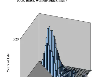
in the three decades between ages 20 and 50. The graphic representation of Appendix Table B appears in Figure 4 below.
Figure 4: Origin and destination of sex difference in life expectancy (U.S. Black women-Black men)
0 10 25 40 55 70 85 100
0 20
45 70
95
0.00 0.20
Y
ear
s of
L
if
e
Origin Age (x)
Destination Age (i)
Source: data in Table 1.
The total for each column gives the total difference in person-years lived in each destination age group i to i+n. In effect, one sums on origin age x rather than on destination age i as in equation 9b above.
(
)
(
)
(
)
[
(
(
)
)
(
(
)
)
]
.0 0,
0 0 0
∑
∑
∑
Ω = − = + + + Ω = − ⋅ − − ⋅ + − ⋅ = = − = − i n i n x a n x i n b n x i n n x a x i n b x i n x a i n b i n i i a i n b i n a b e e l e e l e e l L L e e (10)Summing over x as in equation 10, each iteration beginning from x = 0 contains a term for the current age group minus an equivalent term for the next age group. The next step in the summation then includes the earlier second term as the new first term. Each term beyond the first age group cancels out by being added once and subtracted once. The term added in the final iteration of the sum cancels out the "direct effect" or temporary life expectancy for the age group itself. Only the first term,
(
)
, 1 1 1 0 0 0 − ⋅ = −⋅ n ai
b i n a i n b i n L L e e l
"survives" the summation.
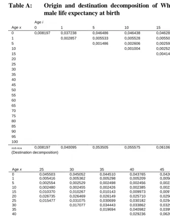
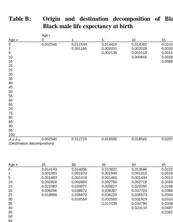
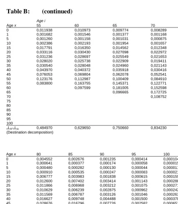
Thus equations 9b and 10 form a "bridge" between origin-decomposition and destination-decomposition of a difference in life expectancies. Tables A and B in the Appendix actually contain two-dimensional origin/destination decomposition matrices of differences in life expectancy, rather than single vectors that attribute the difference either to ages of origin or ages of destination. From these tables, one may inspect the share of any difference in life expectancy that originated in any particular age group,
and that was lived in any other particular age group. Summing in one direction
References
Andreev, Evgeni M. 1982. Method component v analize prodoljitelnosty zjizni [Method of components in analysis of length of life]. Vestnik Statistiki 9:42-7.
Arriaga, Eduardo E. 1984. Measuring and explaining the change in life expectancies.
Demography 21:83-96.
Chiang, Chin Long. 1984. The Life Table and its Applications. New York: Wiley.
Das Gupta, Prithwis. 1978. A general method of decomposing a difference between two rates into several components. Demography 15:99-112.
---. 1994. Standardisation and decomposing of rates from cross-classified data.
Genus 50(3-4): 171-196.
Pollard, John H. 1982. The expectation of life and its relationship to mortality. Journal
of the Institute of Actuaries 109(part II): 225-40.
---. 1988. On the decomposition of changes in expectation of life and differentials in life expectancy. Demography 25: 265-276.
Pressat, Roland. 1985. Contribution des écarts de mortalité par age à la difference des vies moyennes. Population 40:765-70.
Preston, Samuel H., Patrick Heuveline & Michel Guillot 2001. Demography:
Measuring and Modeling Population Processes. Blackwell Publishers Inc.,
Massachusetts, USA.
Shkolnikov, Vladimir, Tapani Valkonen, Alexander Begun & Evgueni Andreev. 2001. Measuring inter-group inequalities in length of life. Genus 57(3-4):33-62.
Vaupel, James W. 1986. How change in age-specific mortality affects life expectancy.
Population Studies 40: 147-57.
Vaupel, James W. & Vladimir Canudas-Romo. 2002. Decomposing demographic change into direct vs. compositional components. Demographic Research 7: 1-14.
---. 2003. Decomposing change in life expectancy: a bouquet of formulas in honor of Nathan Keyfitz´s 90th birthday. Demography 40(2): 201-216.
Appendix
Table A: Origin and destination decomposition of White men minus Black male life expectancy at birth
Age i
Age x 0 1 5 10 15 20
0 0,008197 0,037238 0,046486 0,046438 0,046283 0,045936
1 0,002857 0,005533 0,005528 0,005509 0,005468
5 0,001486 0,002606 0,002598 0,002578
10 0,001004 0,002522 0,002503
15 0,004148 0,010469
20 0,012501
25
30
35
40
45
50
55
60
65
70
75
80
85
90
95
100
nLib-nLia 0,008197 0,040095 0,053505 0,055575 0,061060 0,079455
(Destination decomposition)
Age x 25 30 35 40 45 50
0 0,045503 0,045052 0,044510 0,043765 0,042641 0,040994
1 0,005416 0,005362 0,005298 0,005209 0,005075 0,004879
5 0,002554 0,002529 0,002498 0,002456 0,002393 0,002300
10 0,002480 0,002455 0,002426 0,002385 0,002323 0,002233
15 0,010370 0,010267 0,010143 0,009973 0,009716 0,009340
20 0,026735 0,026469 0,026149 0,025710 0,025047 0,024075
25 0,015477 0,031075 0,030699 0,030182 0,029402 0,028259
30 0,017077 0,034443 0,033862 0,032984 0,031699
35 0,019694 0,040982 0,039918 0,038358
40 0,029236 0,062060 0,059625
45 0,048091 0,100982
50 0,072424
55
60
65 70 75 80 85 90 95 100
nLib-nLia nLia 0,108535 0,140285 0,175860 0,223760 0,299650 0,415170
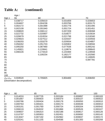
Table A: (continued)
Age i
Age x 55 60 65 70 75
0 0,038717 0,035619 0,031659 0,026653 0,020613
1 0,004607 0,004238 0,003766 0,003170 0,002451
5 0,002172 0,001998 0,001776 0,001495 0,001156
10 0,002109 0,001940 0,001724 0,001451 0,001122
15 0,008820 0,008112 0,007209 0,006068 0,004691
20 0,022732 0,020907 0,018577 0,015634 0,012086
25 0,026679 0,024534 0,021796 0,018340 0,014175
30 0,029923 0,027512 0,024437 0,020559 0,015885
35 0,036203 0,033279 0,029554 0,024857 0,019201
40 0,056262 0,051703 0,045902 0,038594 0,029800
45 0,095250 0,087490 0,077636 0,065242 0,050341
50 0,145821 0,133841 0,118674 0,099643 0,076801
55 0,090226 0,174419 0,154484 0,129558 0,099704
60 0,100234 0,182177 0,152560 0,117184
65 0,085088 0,146845 0,112568
70 0,087781 0,147292
75 0,083874
80 85 90 95
100
nLib-nLia 0,559520 0,705825 0,804460 0,838450 0,808945
(Destination decomposition)
Andreev's
Age x 80 85 90 95 100 nεx
0 0,014024 0,007735 0,003184 0,000897 0,000183 0,672325
1 0,001667 0,000920 0,000379 0,000107 0,000022 0,077460
5 0,000786 0,000434 0,000178 0,000050 0,000010 0,034054
10 0,000763 0,000421 0,000173 0,000049 0,000010 0,030094
15 0,003191 0,001760 0,000724 0,000204 0,000042 0,115248
20 0,008219 0,004532 0,001866 0,000526 0,000107 0,271873
25 0,009637 0,005314 0,002188 0,000617 0,000126 0,288500
30 0,010797 0,005953 0,002451 0,000692 0,000142 0,288416
35 0,013047 0,007192 0,002962 0,000837 0,000172 0,306256
40 0,020241 0,011155 0,004596 0,001300 0,000268 0,410742
45 0,034169 0,018824 0,007758 0,002198 0,000455 0,588435
50 0,052072 0,028670 0,011823 0,003359 0,000700 0,743827
55 0,067497 0,037133 0,015326 0,004371 0,000920 0,773639
60 0,079178 0,043515 0,017980 0,005152 0,001098 0,699078
65 0,075906 0,041671 0,017238 0,004965 0,001072 0,485352
70 0,099095 0,054336 0,022506 0,006519 0,001427 0,418954
75 0,121230 0,066373 0,027536 0,008032 0,001787 0,308832
80 0,047481 0,052262 0,021715 0,006376 0,001441 0,129275
85 0,006925 0,000972 0,000286 0,000065 0,008249
90 -0,012741 -0,012271 -0,002758 -0,027770
95 -0,010009 -0,006805 -0,016814
100 -0,005173 -0,005173
nLib-nLia 0,659000 0,395125 0,148815 0,024255 -0,004690 6,600852
(Destination decomposition)
Table B: Origin and destination decomposition of Black female minus Black male life expectancy at birth
Age i
Age x 0 1 5 10 15 20
0 0,002540 0,011544 0,014410 0,014392 0,014353 0,014263
1 0,001166 0,002031 0,002028 0,002023 0,002010
5 0,002139 0,001519 0,001515 0,001506
10 0,000605 0,002870 0,002852
15 0,008995 0,021262
20 0,019037 25
30 35 40 45 50 55 60 65 70 75 80 85 90 95
100
nLib-nLia 0,002540 0,012710 0,018580 0,018545 0,029755 0,060930
(Destination decomposition)
Age x 25 30 35 40 45 50
0 0,014143 0,014006 0,013831 0,013586 0,013211 0,012668
1 0,001993 0,001974 0,001949 0,001915 0,001862 0,001785
5 0,001493 0,001478 0,001460 0,001434 0,001394 0,001337
10 0,002828 0,002800 0,002765 0,002716 0,002641 0,002532
15 0,021083 0,020877 0,020617 0,020250 0,019692 0,018880
20 0,039256 0,038872 0,038387 0,037703 0,036661 0,035148
25 0,018999 0,036679 0,036220 0,035573 0,034588 0,033158
30 0,016559 0,032500 0,031919 0,031034 0,029747
35 0,017030 0,034799 0,033833 0,032427
40 0,023110 0,048724 0,046695
45 0,038215 0,080788
50 0,060389 55
60 65 70 75 80 85 90 95
100
nLib-nLia 0,099795 0,133245 0,164760 0,203005 0,261855 0,355555
Table B: (continued)
Age i
Age x 55 60 65 70 75
0 0,011938 0,010973 0,009774 0,008289 0,006493
1 0,001682 0,001546 0,001377 0,001168 0,000915
5 0,001260 0,001158 0,001031 0,000875 0,000685
10 0,002386 0,002193 0,001954 0,001657 0,001298
15 0,017791 0,016350 0,014562 0,012348 0,009670
20 0,033116 0,030430 0,027098 0,022972 0,017985
25 0,031236 0,028697 0,025549 0,021653 0,016946
30 0,028020 0,025738 0,022909 0,019411 0,015186
35 0,030540 0,028048 0,024960 0,021143 0,016536
40 0,043970 0,040372 0,035918 0,030416 0,023778
45 0,076053 0,069804 0,062078 0,052541 0,041045
50 0,123176 0,112987 0,100409 0,084910 0,066254
55 0,083800 0,163755 0,145371 0,122771 0,095625
60 0,097599 0,181005 0,152598 0,118576
65 0,096665 0,172725 0,133840
70 0,108752 0,184768
75 0,111854
80 85 90 95
100
nLib-nLia 0,484970 0,629650 0,750660 0,834230 0,861455
(Destination decomposition)
Andreev's
Age x 80 85 90 95 100 nεx
0 0,004552 0,002676 0,001235 0,000414 0,000104 0,209397
1 0,000641 0,000377 0,000174 0,000058 0,000015 0,028689
5 0,000480 0,000282 0,000130 0,000044 0,000011 0,021232
10 0,000910 0,000535 0,000247 0,000083 0,000021 0,033891
15 0,006777 0,003983 0,001838 0,000615 0,000155 0,235748
20 0,012600 0,007402 0,003414 0,001143 0,000288 0,401513
25 0,011866 0,006968 0,003212 0,001075 0,000271 0,342691
30 0,010629 0,006239 0,002875 0,000962 0,000242 0,273971
35 0,011569 0,006787 0,003126 0,001046 0,000263 0,262108
40 0,016627 0,009748 0,004488 0,001500 0,000378 0,325724
45 0,028676 0,016796 0,007726 0,002582 0,000651 0,476955
50 0,046220 0,027029 0,012414 0,004144 0,001045 0,638977
55 0,066559 0,038827 0,017793 0,005931 0,001497 0,741929
60 0,082284 0,047842 0,021856 0,007270 0,001838 0,710868
65 0,092545 0,053594 0,024394 0,008095 0,002049 0,583906
70 0,127185 0,073285 0,033198 0,010982 0,002785 0,540955
75 0,169970 0,097278 0,043785 0,014421 0,003667 0,440975
80 0,096134 0,122217 0,054566 0,017874 0,004560 0,295351
85 0,056323 0,057151 0,018610 0,004766 0,136849
90 0,021893 0,016084 0,004132 0,042109
95 0,003269 0,001291 0,004560
100 -0,002389 -0,002389
nLib-nLia 0,786225 0,578190 0,315515 0,116200 0,027640 6,746010
(Destination decomposition)