A Recursive Method for Structural Learning of Directed Acyclic Graphs

A Recursive Method for Structural Learning of Directed Acyclic

Graphs

Xianchao Xie [email protected]

Zhi Geng [email protected]

School of Mathematical Sciences, LMAM Peking University

Beijing 100871, China

Editor: Marina Meila

Abstract

In this paper, we propose a recursive method for structural learning of directed acyclic graphs (DAGs), in which a problem of structural learning for a large DAG is first decomposed into two problems of structural learning for two small vertex subsets, each of which is then decomposed recursively into two problems of smaller subsets until none subset can be decomposed further. In our approach, search for separators of a pair of variables in a large DAG is localized to small subsets, and thus the approach can improve the efficiency of searches and the power of statistical tests for structural learning. We show how the recent advances in the learning of undirected graphical models can be employed to facilitate the decomposition. Simulations are given to demonstrate the performance of the proposed method.

Keywords: Bayesian network, conditional independence, decomposition, directed acyclic graph, structural learning

1. Introduction

Directed acyclic graphs (DAGs), also known as Bayesian networks, are frequently used to represent independencies, conditional independencies and causal relationships in a complex system with a large number of random variables (Lauritzen, 1996; Cowell et al., 1999; Pearl, 2000; Spirtes et al., 2000). Structural learning of DAGs from data is very important in applications to various fields, such as medicine, artificial intelligence and bioinformatics (Jordan, 2004; Engelhardt et al., 2006).

variable subsets such that u and v are independent conditionally on S. A systematic way of searching for separators in increasing order of cardinality was proposed by Spirtes and Glymour (1991). The PC algorithm limits possible separators to vertices that are adjacent to u and v (Pearl, 2000; Spirtes et al., 2000). Kalisch and B ¨uhlmann (2007) showed that the PC algorithm is asymptotically consistent even when the number of vertices in a DAG grows at a certain rate as the sample size increases.

In this paper, we propose a recursive algorithm in which a problem of structural learning for a large DAG is split recursively into problems of structural learning for small vertex subsets. Our algorithm can be depicted as a binary tree whose top node is the full set of all vertices or variables and whose other nodes are proper subsets of the vertex set at its parent node. The algorithm mainly consists of two steps: the top-down step and the bottom-up step. First at the top-down step, the full set of all variables at the top is decomposed into two small subsets, each of which is decomposed recursively into two smaller subsets until each node cannot be decomposed further at the bottom of the tree. At each step, the decomposition is achieved by learning an undirected graph known as independence graph for a variable subset. Next at the bottom-up step, subgraphs (called skeletons) of leaf nodes are first constructed, and then a pair of child subgraphs are combined together into a large subgraph at their parent node until the entire graph is constructed at the top of the tree. In the algorithm, search for separators in a large graph is localized to small subgraphs. Statistical test is used to determine a skeleton as in the IC algorithm (Verma and Pearl, 1990) and the PC algorithm (Spirtes, 2000). By recursively decomposing the full variable set into small subsets, this algorithm can improve the efficiency of search for separators in structural learning, and it can also make statistical tests more powerful. We also discuss that several methods of learning undirected graphical models (Castelo and Roverato, 2006; Schmidt et al., 2007) can be used to facilitate the decomposition. Finally, we provide simulation results to show the performance of our method.

Section 2 gives notation and definitions. In Section 3, we first present the main theoretical results and then discuss the realization of the algorithm in detail, and we also introduce how the recent advances in various related fields can be used to improve the proposed method. In Section 4, we first use an example to illustrate our approach for learning the equivalence class of a DAG in detail, then we give numerical evaluations of its performance for several networks, and finally we discuss the computational complexity of our recursive algorithm. Conclusion is given in Section 5. The proofs of our main results are presented in Appendix.

2. Notation and Definitions

Let~GV = (V, ~EV)denote a DAG where V ={X1, . . . ,Xn}is the vertex set and~EV the set of directed edges. A directed edge from a vertex u to a vertex v is denoted byhu,vi. We assume that there is no directed loop in ~GV. We say that u is a parent of v and v is a child of u if there is a directed edgehu,vi, and denote the set of all parents of a vertex v by pa(v) and the set of all children of

v by ch(v). We say that two vertices u and v are adjacent in ~GV if there is an edge connecting them. A path l between two distinct vertices u and v is a sequence of distinct vertices in which the first vertex is u, the last one is v and two consecutive vertices are connected by an edge, that is, l= (c0=u,c1, . . . ,cm−1,cm=v)wherehci−1,ciiorhci,ci−1iis contained in~EV for i=1, . . . ,m (m≥1), and ci6=cj for all i6= j. We say that u is an ancestor of v and v is a descendant of u if there is a path between u and v inG~V and all edges on this path point at the direction toward v. The set of ancestors of v is denoted as an(v), and we define An(v) =an(v)∪ {v}. A path l is said to be

(1) l contains a “chain”: u→v→w or a “fork” u←v→w where v is in Z, or

(2) l contains a “collider” u→v←w where v is not in Z and no descendant of v is in Z.

Two disjoint sets X and Y of vertices are d-separated by a set Z if Z d-separates every path from any vertex in X to any vertex in Y ; We call Z a d-separator of X and Y . InG~V, a collider u→v←w is called a v-structure if u and w are non-adjacent inG~V.

Let ¯GV = (V,E¯V)denote an undirected graph where ¯EV is a set of undirected edges. An undi-rected edge between two vertices u and v is denoted by(u,v). An undirected graph is called com-plete if any pair of vertices is connected by an edge. Define a moral graph ¯G_Vmfor a DAGG~V to be an undirected graph ¯Gm

V = (V,E¯V)whose vertex set is V and whose edge set is constructed by marrying parents and dropping directions, that is, ¯EV ={(u,v): hu,viorhv,ui ∈~EV} ∪ {(u,v): (u,w,v)forms a v-structure}(Lauritzen, 1996). An undirected edge added for marrying parents is called a moral edge.

For an undirected graph, we say that vertices u and v are separated by a set of vertices Z if each path between u and v passes through Z. We say that two disjoint vertex sets X and Y are separated by Z if Z separates every pair of vertices u and v for any u∈X and v∈Y . We call (A,B,C) a decomposition of ¯GV if

(1) A∪B∪C=V , and

(2) C separates A and B in ¯GV.

Note that the above decomposition does not require that the separator C is complete, which is required for weak decomposition defined by Lauritzen (1996).

For a set K ⊆V , we say that an undirected graph ¯GK is an undirected independence graph for a DAG ~GV if that a set Z separates X and Y in ¯GK implies that Z d-separates X and Y in

~

GV. An undirected independence graph is minimal if the proper subgraph obtained by deleting any edge is no longer an undirected independence graph. The moral graph ¯G_Vm is the minimal undirected independence graph forG~V with K =V (Lauritzen, 1996). It can also be obtained by connecting each vertex u with all vertices in its Markov blanket Mb(u), which is the minimal set by which u are d-separated from the remaining set in V (that is, V\[Mb(u)∪ {u}]). For a subset

K ⊆V , the Markov blanket for a vertex u∈K can be defined similarly, that is, it is the

mini-mum set that is contained in K and d-separates u from the remaining set in K. When K=V ,

it is easy to verify Mb(u) =pa(u)∪ch(u)∪pa(ch(u)). Define the local skeleton for a variable set K ⊆V with respect to ~GV as an undirected graph ¯LK(K,E) where K is the vertex set and

E ={(u,v): no subset S of K d-separates u and v inG~V} is the edge set. Note that though both minimal undirected independence graphs and local skeletons are undirected graphs and defined on the same vertex subset, they may be different. According to the definition of a minimal undirected independence graph, the absence or presence of an edge between u and v in the minimal undirected independence graph over K ⊆V depends on whether its two vertices are d-separated by the

re-maining set K\ {u,v} in ~GV, while an edge between u and v in the local skeleton is determined by whether there exists a subset of K that can d-separate u and v in ~GV. Thus the edge set of the minimal undirected independence graph contains the edge set of the local skeleton.

*

+

,

-.

/

0

1

(a) The DAG~GV

*

+

,

-.

/

0

1

(b) The moral graph ¯Gm V

a

c

d

b

c

d

e

f

g

h

(c) One decomposition based on ¯Gm_V

*

+

,

(d) A local skeleton

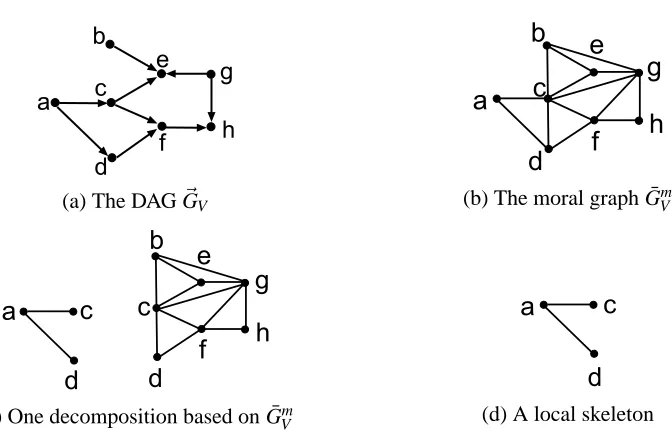
Figure 1: A directed graph, a moral graph, a decomposition and a local skeleton.

are called Markov equivalent if they induce the same conditional independence restrictions. Two DAGs are Markov equivalent if and only if they have the same global skeleton and the same set of

v-structures (Verma and Pearl, 1990). An equivalence class of DAGs consists of all DAGs which are

Markov equivalent, and it is represented as a partially directed graph (PDAG) where the directed edges represent arrows that are common to every DAG in the Markov equivalence class, while an undirected edge represents that the edge is oriented one way in some member of the Markov equivalence class, and is oriented the other way in some other member. Therefore the goal of structural learning is to construct a PDAG to represent the equivalence class.

Example 1. Consider the DAG in Figure 1 (a). b→e←c, b→e←g, c→ f ←d, c→e←

g and f → h← g are v-structures. A path l = (c,a,d) is d-separated by vertex a, while the path l0 = (c,f,h,g) is d-separated by an empty set. We have an(e) ={a,b,c,g} and An(e) =

{a,b,c,g,e}. The Markov blanket of c is Mb(c) ={a,b,d,e,f,g}, which d-separates c and the remaining set{h}. The moral graph ¯Gm_V is given in Figure 1 (b), where edges(b,c),(b,g),(c,g), (c,d) and(f,g) are moral edges. Note that the set{c,d} separates{a} and{b,e,f,g,h} in ¯G_Vm, thus({a},{b,e,f,g,h},{c,d})forms a decomposition of the undirected graph ¯Gm_V, the decomposed undirected independence subgraphs for{a,c,d}and{b,c,d,e,f,g,h}are shown in Figure 1 (c). The graph in Figure 1 (d) is the local skeleton ¯LK(K,E)for K={a,c,d}because we have c and d are d-separated by{a}inG~V. Note that the minimal undirected independence graph for{a,c,d} in Figure 1(c) coincides with its local skeleton in Figure 1 (d), which does not hold in general. For example, the local skeleton for K={c,e,g}does not have the edge(c,g), while the corresponding minimal undirected independence graph is complete.

Given a DAGG~V, a joint distribution or density of variables X1, . . . ,XN is

P(x1,· · ·,xN) = N

∏

where P(xi|pai) is the conditional probability or density of Xi given pa(Xi) = pai. The DAGG~V and the joint distribution P are said to be compatible (Pearl, 2000) and P obeys the global directed Markov property of G~V (Lauritzen, 1996). Let X Y denote the independence of X and Y , and

X Y|Z the conditional independence of X and Y given Z. In this paper, we assume that all

inde-pendencies of a probability distribution of variables in V can be checked by d-separations of G~V, called the faithfulness assumption (Spirtes et al., 2000), which means that all independencies and conditional independencies among variables can be represented by~GV. As a consequence, we also use to denote the d-separation in DAGs.

3. A Recursive Method for Structural Learning of a DAG

In this section, we first present theoretical results in this paper and then we apply these results to structural learning of a DAG and show how the problem of searching for d-separators over the full set of all vertices can be recursively split into the problems of searching for d-separators over smaller subsets of vertices. We also discuss how to learn from data the undirected independence graphs which are used to achieve the recursive decomposition at each recursive step.

3.1 Theoretical Results and Recursive Algorithm for Structural Learning

Below we first give two theorems based on which we propose the recursive algorithm for structural learning of DAGs.

Theorem 1. Suppose that A B|C in a DAG G~V. Let u∈A and v∈A∪C. Then u and v are

d-separated by a subset of A∪B∪C if and only if they are d-separated by a subset of A∪C.

According to Theorem 1, we can see that all edges falling in A or crossing A and C in the local skeleton ¯L(K,E) with K =A∪C∪B can be validly recovered from the marginal distribution of

variables in A∪C. Note that such a local skeleton over K can be used to recover the entire DAG

over V even if there may not exist a marginalized DAG over K (Richardson and Spirtes, 2002). Theorem 2. Suppose that A B|C in a DAGG~V. Let u and v be two vertices both of which are contained in the separator C. Then u and v are d-separated by a subset of A∪B∪C if and only if

they are d-separated by a subset of A∪C or by a subset of B∪C.

According to Theorem 2, the existence of an edge falling into the separator C in the local skele-ton ¯L(K,E)with K=A∪C∪B can be determined from the marginal distribution of A∪C or the

marginal distribution of B∪C.

Note that the union set K=A∪B∪C in Theorems 1 and 2 may be a subset of the full set V

(that is, K⊆V ), and they are more general results than Theorem 1 presented in Xie et al. (2006),

which requires that the union set K equals V (that is, K=A∪B∪C=V ). These two theorems

can guarantee that, for any partition(A,B,C)of a vertex set K ⊆V that satisfies A B|C, two

non-adjacent vertices u and v in K are d-separated by a subset S of K in G~V if and only if they are

d-separated by a subset S0 of either A∪C or B∪C inG~V. Therefore, we have the following result. Theorem 3. Suppose that A B|C in a DAG G~V. Then the local skeleton ¯LK = (K,EK) can be constructed by combining local skeletons ¯LA∪C = (A∪C,EA∪C) and ¯LB∪C= (B∪C,EB∪C) as follows:

(1) the vertex set K=A∪C∪B and

Based on these theorems, we propose a recursive algorithm for learning the structure of a DAG. Our algorithm has a series of operations on a binary tree. The top node of the tree is the full set of all variables, the leaves of the tree are subsets of variables which cannot be decomposed, and the variable set of each parent node in the binary tree is decomposed into two variable sets of its two children. Our algorithm consists of two steps: the top-down step for decomposing the full set of all variables into subsets as small as possible, and the bottom-up step for combining local skeletons into the global skeleton. At the top-down step, a variable set is decomposed into two subsets whenever a conditional independence A B|C is found, and this decomposition is repeated

until no new decomposition can be found. The decomposition at each step is done by learning an undirected independence graph over the vertex subset at the tree node, which will be discussed in Subsection 3.3. At the bottom-up step, two small skeletons are combined together to construct a larger skeleton, and the combination is repeated until the global skeleton is obtained. The entire process is formally described in the following algorithm.

Main Algorithm (The recursive decomposition for structural learning of DAGs)

1. Input: a target variable set V ; observed data D.

2. Call DecompRecovery (V , ¯LV) to get the global skeleton ¯LV and a separator list

S

3. For each d-separator Suv in the separator list

S

skeleton and w is not contained in the separator Suv.

4. Apply Meek’s rule (Meek, 1995) to obtain a DAG in the Markov equivalence class: we orient other edges if each opposite of them creates either a directed cycle or a new v-structure. The Markov equivalence class can be obtained by collecting all possible DAGs.

5. Output: the equivalence class of DAGs.

PROCEDURE DecompRecovery (K, ¯LK)

1. Construct an undirected independence graph ¯GK;

2. If ¯GKhas a decomposition(A,B,C)

Then

• For each pair(u,v)of u∈A and v∈B, save(u,v,Suv=C)to the d-separator list

S

• DecompRecovery (A∪C, ¯LA∪C);

• DecompRecovery (B∪C, ¯LB∪C);

• Set ¯LK= CombineSubgraphs ( ¯LA∪C, ¯LB∪C)

Else

• Construct the local skeleton ¯LK directly (such as using the IC algorithm): Start with a complete undirected graph over K.

For any vertex pair(u,v)in the set K, if there exists a subset Suv of K\ {u,v}such that

3. RETURN ( ¯LK).

FUNCTION CombineSubgraphs ( ¯LU, ¯LV)

1. Combine ¯LU = (U,EU) and ¯LV = (V,EV) into an undirected graph ¯LU∪V = (U∪V,EU∪V) where

EU∪V = (EU∪EV)\ {(u,v): u,v∈U∩V and(u,v)6∈EU∩EV};

2. Return(¯LU∪V).

As shown in the main algorithm, the equivalence class of~GV can be constructed by first calling DecompRecovery (V , ¯LV) to get the skeleton, then recover all v-structures using the d-separator list

S

A binary decomposition tree is used in DecompRecovery to describe our algorithm simply and clearly. In our implementation, we use a junction tree to decompose a graph into several subgraphs simultaneously and to find the corresponding separators. It is known that the junction tree may not be unique, and thus we may have multiple decompositions. In theory, we prefer to use the junction tree with the minimum tree width. However, this is known to be an NP hard problem (Arnborg et al., 1987); therefore, we may use some sub-optimal method to consruct a junction tree for an undirected graph (Jensen and Jensen, 1994; Becker and Geiger, 2001). For example, two most well-known algorithms are the lexicographic search (Rose et al., 1976) and the maximum cardinality search (Tarjan and Yannakakis, 1984), whose computational expenses are O(ne) and

O(n+e)respectively, where e is the number of edges in the graph. Especially, the latter method is used in our implementation. According to our experiences, the junction tree obtained by either method usually leads to very efficient decompositions.

In the recursive algorithm, statistical tests are used only at the top-down step but not at the bottom-up step. Thus the data sets used for statistical tests can be reduced into marginal data sets with decomposition of graphs. In this way, we only need to pass through small marginal data sets for statistical tests of subgraphs and need not pass through the full data set for every statistical test. Other algorithms (such as the PC algorithm) can be used to replace the IC algorithm to improve the performance of constructing the local skeleton ¯LK in DecompRecovery.

3.2 Tests of Conditional Independence

Conditional independence test of two variables u and v given a set C of variables is required at Step 1 and the ‘Else’ part of Step 2 of Procedure DecompRecovery to construct an undirected independence graph and a local skeleton respectively. Null hypothesis H0is u v|C and alternative H1is that H0 may not hold. Generally we can use the likelihood ratio test statistic

G2=−2 logsup{L(θ|D)under H0} sup{L(θ|D)under H1}

,

Let Xkbe a vector of variables and N be the sample size. For the case of a Gaussian distribution, the test statistic for testing Xi Xj|Xkcan be simplified to

G2 = −N×log(1−corr2(Xi,Xj|Xk)) = N×logdet(

ˆ

Σ{i,k}{i,k})det(Σˆ{j,k}{j,k}) det(_Σˆ_{{i,j,k}{i,j,k})det(Σ}ˆ_k,k) ,

which has an asymptoticχ2distribution with d f=1. Actually, the exact null distribution or a better approximate distribution of G2 can be obtained based on Bartlett decomposition, see Whittaker (1990) for more detailed discussion on this.

For the discrete case, let N_smbe the observed frequency in a cell of Xs=m where s is an index set of variables and m is a category of variables Xs. For example, N_{i jk}abc denotes the frequency of

Xi=a, Xj=b and Xk=c. The G2statistic for testing Xi Xj|Xkis then given by

G2=2

∑

N_{i jk}abclogN abc i jkNkc

N_ikacNbc_jk,

which is asymptotically distributed as aχ2distribution under H0with degree of freedom df= (#(Xi)−1)(#(Xj)−1)

∏

Xl∈Xk

#(Xl),

where #(X)is the number of categories of variable X .

For discrete data, the size of conditional variable sets cannot be so large that independence tests become inefficient. Thus the algorithm restricts the cardinality of conditioning sets. There are many methods that can be used to find a small conditioning set, such as a forward selection of variables. With the recursive decomposition, independence tests are localized to smaller and smaller subsets of variables, and thus the recursive algorithm has higher power for statistical tests.

3.3 Constructing Undirected Independence Graphs

In this subsection, we discuss how to construct undirected independence graphs at Step 1 of Proce-dure DecompRecovery. At first we call DecompRecovery with the full set V as the input argument, and construct an undirected independence graph ¯GV at Step 1. Then at each recursive calling, to construct a local undirected independence graph ¯GK with a subset K (say K=A∪C) as the input argument, we shall present a theoretical result based on which we only need to check edges over the separator C without need of testing conditional independencies between any pair of variables in A and between any pair of variables crossing A and C.

by A∪C in the previous graph ¯GA∪B∪C and then only pairs of vertices contained in C need to be checked via conditional independence tests.

Theorem 4. Suppose that the distribution of V =A∪B∪C is positive and has the conditional

independence A B|C. Then for any u in A and any v in A∪C, we have that u v|[(A∪C)\ {u,v}]if and only if u v|[(A∪B∪C)\ {u,v}].

Note that Theorems 1 and 4 are different. The former is used to determine an edge in a DAG, and the latter is used to determine an edge in an undirected independence graph. According to this theorem, there exists an edge(u,v)in the minimal undirected independence graph ¯GA∪C for u in A and v in A∪C if and only if there exists an edge(u,v)in the minimal undirected independence graph

¯

GA∪B∪C. Thus given an undirected independence graph ¯GA∪B∪C obtained in the preceding step, an undirected independence graph ¯GA∪Chas the same set of edges as ¯GA∪B∪Ceach of which has at least one vertex in A, but all of possible edges within the separator C need to be checked for ¯GA∪C.

When there is a large number of variables and a small sample size, it is infeasible or statisti-cally unstable to test an independence between two variables conditionally on all other variables, and this problem is more serious when variables are discrete. Many current methods for learning undirected graphical models can also be used in our algorithm. For example, procedures based on limited-order partial correlations (Wille and B ¨uhlmann, 2004; Castelo and Roverato, 2006) are rather suitable and can be even used in the case where the number of variables is larger than the number of samples. Another way of learning undirected independence graphs is to apply current available Markov blanket learning algorithms. By connecting each vertex with those in its Markov blanket, an independence graph is then obtained. Indeed, it is neither new nor uncommon to learn the Markov blanket as either an initial step for learning a DAG or as a special problem of interest. Koller and Sahami (1996) developed a method for feature selection which employs the concept of Markov blanket. Margaritis and Thrun (1999) proposed a two-phase algorithm to first identify a Markov blanket for each variable and then obtain a DAG by connecting vertices in a maximally consistent way. Tsamardinos et al. (2003) proposed a method that can soundly identify all Markov blankets and scale-up to a graph with thousands of variables.

Another particular method for learning the undirected independence graph may use Lasso-type estimators (Tibshirani, 1996; Meinshausen and B ¨uhlmann, 2006; Zhao and Yu, 2006; Wainwright et al., 2006). We can apply Lasso method to select a neighborhood set of a vertex which contains the Markov blanket of the vertex. Schmidt et al. (2007) developed a new method of learning structure of a DAG. Note that it is not necessary to learn neighborhoods exactly in our algorithm, and there may be extra edges in our undirected independence graph.

4. Illustration and Evaluation of the Recursive Algorithm

In this section, we first illustrate the recursive algorithm step by step via a concrete example and then show simulation results to evaluate its performance.

4.1 Illustration of the Recursive Algorithm

compare the recursive algorithm with the decomposition algorithm proposed in Xie et al. (2006), in which an entire undirected independence graph is first constructed and then it is decomposed into many small subgraphs at one step instead of recursive steps. We show that, in our algorithm, search for separators is localized to smaller vertex subsets than those obtained by using the decomposition algorithm.

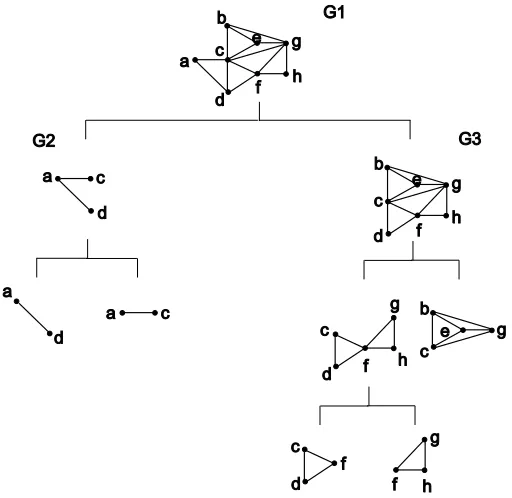
Example 1. (Continued) Consider again the DAG~GV = (V, ~EV)in Figure 1 (a). We call Procedure DecompRecovery to construct the global skeleton over V . At the top-down step (that is, at the ‘Then’ part of Step 2 in DecompRecovery), we construct the binary tree shown in Figure 2. At the top of the binary tree, the first decomposition is done by splitting the full vertex set V in G1 (that is, the moral graph) into two subsets{a,c,d}and{b,c, . . . ,h}with the separator{c,d}. Next we learn the undirected independence graphs G2 and G3 for the two subsets separately. To construct the subgraphs G2 and G3, by Theorem 5, we only need to check the edge (c,d) in the separator

{c,d}, and other edges in G2and G3can be obtained directly from G1. Repeat this procedure until no further decomposition is possible. Finally we get the entire binary tree T as shown in Figure 2, where each leaf node is a complete graph and cannot be decomposed further.

-* -+ -, . / 0 1 2 3 4 5 . 0 1 / 0 1 2 3 4 5 . 0 . 1 / 0 2 4 0 3 4 5 0 1 3 3 4 5 1

Figure 2: The binary tree T obtained at the top-down step (at ‘Then’ of Step 2).

K2 K1 a c a d c d f f g h b c e g

L3

L6 L5

L4

L1 L2

a b c d

e f

g h

a c d

b c d

e f

g h

a c a

d b

c e

g c

f g h

c d

f f

g h d

Figure 4: Combinations of local skeletons in Procedure CombineSubgraphs.

Before the bottom-up step (that is, the ‘Else’ part of Step 2 in Procedure DecompRecovery), for each leaf node K, we construct a local skeleton over K. For each vertex pair(u,v) in K, we search a separator set Suv in all possible subsets of K\ {u,v}to construct the local skeleton. All local skeletons of leaf nodes are shown in Figure 3. For example, the vertices c and d are adjacent in the local skeleton K1since no vertex set in K1d-separates them, whereas b and g are non-adjacent

in the local skeleton K2since an empty set d-separates them in~GV. At the bottom-up step, calling Function CombineSubgraphs, we combine the local skeletons from the leaf nodes to the root node to form the global skeleton, as shown in Figure 4. For example, local skeletons L1 and L2 are combined to L3, and then L3and L4 are combined to L5, as shown in Figure 4. Similarly, we get the local skeleton L6. At the last step, we combine L5and L6into the global skeleton. Note that the edge(c,d)in L5is deleted at Step 1 of Function CombineSubgraphs since the edge is not contained in L6. After all the combinations are done, we get the global skeleton in Figure 5. We can see that the undirected independence graphs and the local skeletons are different as shown in Figure 2 and Figure 4 respectively and that the former has more edges than the latter.

At Step 2 of Procedure DecompRecovery, we save all separators to the d-separator list

S

S

S

a

b

c

d

e

f

g

h

Figure 5: The global skeleton ¯LV.

a b

c

d e

f g

h

Figure 6: The recovered equivalence class.

b and g in~GV, we can orient b−e−g as b→e←g. After recovering all v-structures, we apply the orientation rule in Meek (1995) and get the desired equivalence class of G~V in Figure 6. In this equivalence class, the undirected edge (a,c) cannot be oriented uniquely because any of its orientation leads to a Markov equivalent DAG.

Below we compare the recursive algorithm with the decomposition algorithm proposed in Xie et al. (2006). We show that theoretically the recursive algorithm can decompose the entire graph into smaller subgraphs than the decomposition algorithm does because the decomposition in the decomposition algorithm is done only once, whereas the recursive algorithm tries to re-decompose undirected independence subgraphs at each recursive step. When there are a lot of v-structures in a DAG, many moral edges can be deleted in construction of a subgraph, and thus the recursive algorithm is more efficient than the decomposition algorithm. The following example illustrates the difference of decompositions obtained by these two algorithms.

Example 2. Consider the DAG in Figure 7. By using the decomposition algorithm proposed in Xie

et al. (2006), a ‘d-separation tree’ is built from an undirected independence graph (that is, the moral graph in this example), and the full variable set is decomposed into three subsets of variables at one time, see Figure 8 (a). By using the recursive algorithm proposed in this paper, we can decompose the graph into four subgraphs in Figure 8 (b), which have smaller subsets of variables. This is because the undirected independence graph over{a,b,c}in Figure 8 (b) is re-constructed and the edge(b,c)is deleted for b c|a.

-,

+

*

_.

. * + , -+ , - - . * + ,

(a) The decomposition algorithm.

- - . * + , -+ , * , + + * * , . * + ,

-(b) The recursive algorithm.

Figure 8: Comparison of two different algorithms for structural learning.

4.2 Simulation Studies

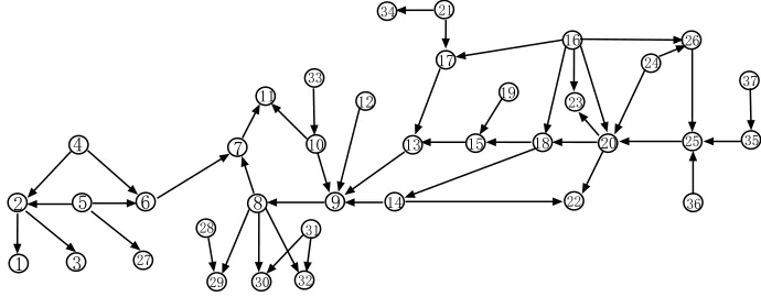
Below we give numerical examples to evaluate the performance of the recursive algorithm. We first present simulation results for the ALARM network, which is a medical diagnostic network and is shown in Figure 9 (Beinlich et al., 1989; Heckerman, 1998). It is a DAG with 37 vertices and 46 edges and it is often used to evaluate performance of learning algorithms. In the following two subsections, we use the ALARM network to do simulation for the Gaussian case and the discrete case separately. Next we show simulation results for several other networks in the final subsection.

+ , -/ 0 1 2 3 +* +, +. +/ +1 +2 +3 ,+ ,, ,-,. ,/ ,0 ,2 ,3 -* -+ -, -. -/ . ++ ,* ,1 -- +-+0 -0 -1

Figure 9: The ALARM network.

4.2.1 THEGAUSSIANCASE

In this subsection, for the underlying DAG of the ALARM network, we generate a sample from a joint Gaussian distribution using a structural equation model of recursive linear regressions, whose coefficients are randomly generated from the uniform distribution in the interval (−1.5,−0.5)∪

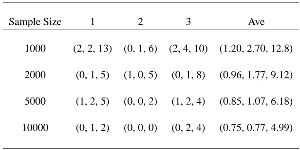
constructed DAG and record the number of extra edges, the number of missing edges and the struc-tural hamming distance (SHD), where SHD is defined as the total number of operations to verify the constructed PDAG to the Markov equivalence class of the underlying DAG, and where the opera-tions may be: add or delete an undirected edge, and add, remove or reverse an orientation of an edge (Tsamardinos et al., 2006). The likelihood ratio test introduced in Subsection 3.2 is used to test the partial correlation coefficient at the significance levelα=0.01. We repeatedly draw n=1000 sets of samples and obtain the average numbers of extra edges, missing edges and SHD from n=1000 simulations. The first 3 simulation results are shown in Table 1 for different sample sizes 1000, 2000, 5000 and 10000. In Table 1, three values in a bracket denote the number of extra edges, the number of missing edges and SHD respectively. The column ‘Ave’ in Table 1 shows the averages of

n=1000 simulations. It can be seen that the algorithm performs better as the sample size increases. From the simulations, we found that most decompositions at the top-down step are correct, and we also found that when coefficients make the faithfulness assumption close to fail (that is, some of the edges only reflect weak or nearly zero associations), the learned PDAG from simulation may not be exactly the same as the underlying PDAG, and most of edge mistakes appear for these edges that represent rather weak associations.

Sample Size 1 2 3 Ave

1000 (2, 2, 13) (0, 1, 6) (2, 4, 10) (1.20, 2.70, 12.8)

2000 (0, 1, 5) (1, 0, 5) (0, 1, 8) (0.96, 1.77, 9.12)

5000 (1, 2, 5) (0, 0, 2) (1, 2, 4) (0.85, 1.07, 6.18)

10000 (0, 1, 2) (0, 0, 0) (0, 2, 4) (0.75, 0.77, 4.99)

Table 1: Extra edges, missing edges, and SHD for the first 3 simulations and averages from 1000 simulations.

Our implementation is based on the Bayesian network toolbox written by Murphy (2001) and the simulations run particularly fast. For a single simulation for all sample sizes N=1000, 2000, 5000, 10000, when conditional independence tests are used to check edges, it costs only around 3 seconds in Matlab 7 on a laptop Intel 1.80GHz Pentium(R)M with 512 MByte RAM running Windows XP.

Alg (Levelα) N = 1000 N = 2000 N = 5000 N = 10000 Ave Time (1.2, 2.4, 12) (1.0, 1.5, 8.2) (0.9, 0.9, 5.8) (0.7, 0.6, 4.6) 2.55 sec

Rec(0.01) (1.0, 1.0, 1.0) (1.0, 1.0, 1.0) (1.0, 1.0, 1.0) (1.0 ,1.0, 1.0) 1.0

Rec(0.05) (3.1, 1.0, 1.5) (3.5, 1.1, 1.7) (4.2, 1.1, 2.2) (4.7, 1.2, 2.3) 1.5

PC(0.01) (1.8, 4.5, 3.5) (2.6, 6.3, 4.7) (2.8, 8.0, 6.0) (4.0, 9.7, 7.2) 21.2

PC(0.05) (2.9, 4.0, 3.5) (4.3, 3.5, 4.7) (6.0, 4.0, 6.2) (8.6, 5.1, 7.3) 24.8

TPDA(0.01) (3.9, 4.1, 3.5) (4.3, 5.7, 4.8) (3.9, 7.5, 6.1) (3.7, 8.5, 6.8) 73.6

TPDA(0.05) (4.4, 3.7, 3.5) (4.7, 5.1, 4.7) (5.7, 4.3, 6.0) (8.5, 4.8, 7.1) 88.3

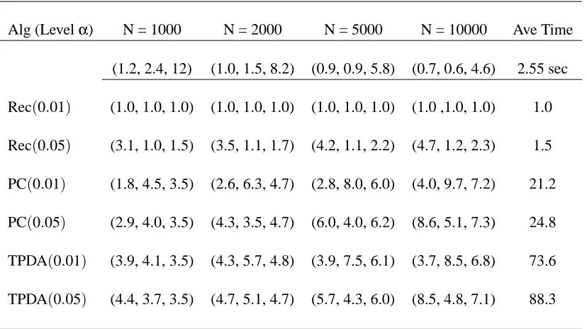
Table 2: Results relative to the recursive algorithm withα=0.01 andα=0.05: extra edges, miss-ing edges, and SHD

which are obtained by dividing their real values by the underlined values in the second row. A relative value larger than 1 denotes that its real value is larger than the corresponding value in the second row. For example, the third row labeled Rec(0.01)with all values equal to 1 shows that our algorithm withα=0.01 has the same results as the second row; the seventh row labeled PC(0.01) shows the relative results for the PC algorithm withα=0.01, where(1.8,4.5,3.5)means the real values as(1.8×1.2,4.5×2.4,3.5×12). The last column labeled ‘Ave Time’ denotes average time cost for one simulation of all 4 sample sizes. In Table 2, all values are larger than 1, which means our algorithm Rec(0.01) has the least number of extra edges, the least number of missing edges and the least SHD, and further it costs the least times.

4.2.2 THEDISCRETECASE

Now we show simulations of the ALARM network for the discrete case where these discrete vari-ables have two to four levels. For every simulation, the conditional probability distribution of each variable Xigiven its parents paiis draw randomly in the following way: for each fixed configuration

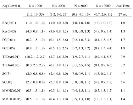
algorithm, we set the parameter max-fan-in (that is, the maximum in-degree) to its true value so that the PC algorithm can run fast. We use the TPDA and the MMHC algorithms that are implemented in the Causal Explorer System (Aliferis et al., 2003) with the default setting. For all algorithms except the SC algorithm, we use two significance levels (α=0.01,α=0.05) in the simulations. For the SC algorithm, the most important parameter to be specified is the number of candidates (the maximum size of potential parent sets), which are set to 5 and 10 separately.

Alg (Levelα) N = 1000 N = 2000 N = 5000 N = 10000 Ave Time

(1.3, 10, 33) (1.2, 6.6, 23) (0.8, 4.0, 16) (0.7, 2.6, 11) 27 sec

Rec(0.01) (1.0, 1.0, 1.0) (1.0, 1.0, 1.0) (1.0, 1.0, 1.0) (1.0, 1.0, 1.0) 1.0

Rec(0.05) (4.0, 0.8, 1.1) (3.6, 0.8, 1.2) (4.8, 0.8, 1.3) (4.9, 0.8, 1.4) 1.3

PC(0.01) (0.2, 1.5, 1.9) (0.1, 1.5, 2.6) (0.2, 1.6, 3.3) (0.1, 1.8, 4.5) 1.7

PC(0.05) (0.8, 1.2, 1.9) (0.5, 1.3, 2.5) (0.7, 1.3, 3.2) (0.7, 1.5, 4.4) 1.9

TPDA(0.01) (10.2, 1.2, 2.7) (2.7, 1.6, 3.0) (1.9, 2.7, 4.1) (0.9, 4.1, 5.8) 0.9

TPDA(0.05) (0.0, 2.5, 2.2) (0.1, 3.9, 3.1) (0.1, 6.5, 4.5) (0.1, 9.9, 6.6) 0.2

SC(5) (2.0, 0.8, 0.8) (2.4, 0.8, 1.0) (3.6, 0.9, 1.1) (4.3, 0.9, 1.4) 4.7

SC(10) (2.2, 0.8, 0.8) (2.7, 0.9, 1.0) (3.8, 0.8, 1.1) (4.2, 0.7, 1.2) 6.6

MMHC(0.01) (0.3, 1.3, 1.1) (0.3, 1.4, 1.1) (0.4, 1.5, 1.1) (0.7, 1.5, 1.2) 1.1

MMHC(0.05) (0.5, 1.2, 1.0) (0.4, 1.3, 1.0) (0.5, 1.3, 1.0) (1.0, 1.3, 1.1) 1.4

Table 3: Results relative to the recursive algorithm withα=0.01 andα=0.05: extra edges, miss-ing edges, and SHD

(excluding an edge that is in the true DAG). For example, the PC and MMHC algorithms have a smaller false positive error; the SC algorithm has a smaller false negative error; and the recursive algorithm has smaller SHD. We also found that choosing a good parameter is also important to achieve an optimal performance for each algorithm. The recursive algorithm seems to work better when we choose a significance levelα=0.01, while for MMHC it is better to chooseα=0.05.

The above comparison is based on results from randomly generated values of parameters of joint distributions. The results may change when different values of these parameters are used. The performance of an algorithm also depends on the structures of a network.

4.2.3 SIMULATIONS OFOTHERNETWORKS

In this subsection we show simulation results for other three networks: Insurance with 27 vertices and 52 edges (Binder et al., 1997), HailFinder with 56 vertices and 66 edges (Abramson et al., 1996) and Carpo with 61 vertices and 74 edges, all of which can be obtained through the online Bayesian network repository (http://www.cs.huji.ac.il/labs/compbio/ Repository). We compare the recursive algorithm with the SC and MMHC algorithms since these two have been extensively compared with many state-of-art algorithms and shown in general outperforming other algorithms by Tsamardinos et al. (2006). In our simulations, the parameter values of the joint distributions are set to the original values from the repository. For each network, 10 data sets are generated, and we give one better result in Table 4 for each algorithm with two criteria (α=0.01 and 0.05 for Rec and MMHC, the number of candidates = 5 and 10 for SC). From the last column ‘Ave Time’ of Table 4, it can be seen that the recursive algorithm is fastest in average CPU time and it also has a better performance in most cases for these networks.

4.3 Complexity Analysis

Below we discuss the complexity of the recursive algorithm proposed in this paper. We mainly focus on the number of conditional independence tests for constructing the equivalence class since decomposition of graphs is a computationally simple task compared to the conditional independence tests. In the recursive algorithm DecompRecovery, two steps (Step 1 for constructing an undirected independence graph ¯GK and the ’Else’ part of Step 2 for constructing a local skeleton ¯LK) involve conditional independence tests, where K is the vertex set of the subgraph. At Step 1, an undirected independence graph can be constructed by testing independence between any pair of variables con-ditionally on other variables, and thus the complexity is O(|K|2_{), where|K|denotes the number of} vertices in the set K. As discussed in Section 3.3, an undirected independence graph ¯GA∪C can be constructed from the previous graph ¯GA∪B∪C by checking only all possible edges within the sepa-rator C. Thus the complexity for constructing an undirected independence graph can be reduced. At Step 2, we construct a local skeleton over a vertex subset K. Suppose that we use the IC al-gorithm. Then the complexity for constructing the local skeleton LK is O(|K|22|K|−2). Below we consider the total expenses and suppose that the full vertex set V is recursively decomposed into

Alg (Levelα) N = 1000 N = 2000 N = 5000 N = 10000 Ave Time Insurance

(2.4, 13, 43) (1.5, 10, 40) (1.3, 7.4, 32) (1.1, 6.7, 27) 16 sec

Rec(0.01) (1.0, 1.0, 1.0) (1.0, 1.0, 1.0) (1.0, 1.0, 1.0) (1.0, 1.0, 1.0) 1.0

SC(5) (1.6, 1.0, 1.0) (2.3, 1.2, 1.2) (2.5, 1.3, 1.3) (2.9, 1.4, 1.5) 6.7

MMHC(0.05) (0.6, 1.3, 1.1) (1.1, 1.4, 1.2) (1.2, 1.5, 1.2) (1.1, 1.4, 1.2) 8.0

Hailfinder

(5.9, 16, 53) (7.1, 14, 47) (8.0, 14, 43) (7.3, 14, 41) 62 sec

Rec(0.01) (1.0, 1.0, 1.0) (1.0, 1.0, 1.0) (1.0, 1.0, 1.0) (1.0, 1.0, 1.0) 1.0

SC(10) (2.0, 1.0, 1.1) (1.8, 1.1, 1.1) (2.0, 1.1, 1.3) (2.1, 0.8, 1.2) 5.6

MMHC(0.05) (1.6, 1.2, 1.1) (1.6, 1.1, 1.0) (1.7, 1.1, 1.2) (1.0, 1.9, 1.2) 17.4

Carpo

(10, 12, 49) (9.0, 5.0, 36) (6.5, 2.6, 21) (6.3, 1.0, 18) 74 sec

Rec(0.01) (1.0, 1.0, 1.0) (1.0, 1.0, 1.0) (1.0, 1.0, 1.0) (1.0, 1.0, 1.0) 1.0

SC(10) (2.3, 0.5, 1.2) (2.6, 0.5, 1.7) (2.8, 0.9, 2.2) (2.3, 1.3, 2.0) 6.6

MMHC(0.05) (2.5, 2.4, 2.1) (2.6, 4.5, 2.6) (3.1, 6.0, 3.4) (3.0, 12, 3.4) 44

Table 4: Results relative to the recursive algorithm for other networks: extra edges, missing edges, and SHD

5. Conclusion

In this paper, we proposed a recursive algorithm for structural learning of DAGs. We first present its theoretical properties, then show its experimental results and compare it with other algorithms. In the recursive algorithm, a structural learning for a large DAG is first split recursively into those for small subgraphs until each subgraph cannot be decomposed further, then we perform local learn-ing for these subgraphs which cannot be decomposed, finally we gradually combine these locally learned subgraphs into the entire DAG. The main problem for structural learning of a DAG is the search for d-separators, which becomes exponentially complicated with the number of vertices in-creases. In the recursive algorithm, all searches for d-separators are localized into subsets of ver-tices. Thus the efficiency of structural learning and the power of statistical tests can be improved by decomposition.

There are several works related to our recursive approach. Friedman et al. (1999) discussed how the idea of recursive decomposition can be used in accelerating their Sparse Candidate algo-rithm, Narasimhan and Bilmes (2005) discussed the application of this idea to find a sub-optimal graphical models by noticing the corresponding decomposition of the Kullback and Leibler diver-gence (Kullback and Leibler, 1951) with respect to the graph separation. Geng et al. (2005) and Xie et al. (2006) proposed the decomposition algorithms for structural learning of DAGs. However, the method proposed in Geng et al. (2005) requires that each separator has a complete undirected graph. Xie et al. (2006) removed the condition, but their algorithm performs decomposition only based on the entire undirected independence graph ¯GV of the full vertex set V and cannot perform decomposition of undirected independence subgraphs. Theorems 1, 2 and 3 in this paper relax this requirement, and they do not require the union set K=A∪B∪C of a decomposition(A,B,C) to be equal to the full vertex set V . Thus the recursive algorithm can delete more edges in undirected independence subgraphs and further decompose them, see Example 2. Theorems 1, 2 and 3 are also useful properties for collapsibility of DAGs.

Now we discuss several potential utilities and further works of the recursive approach. This re-cursive decomposition approach can also be used to localize a learning problem of interest. Suppose that V is the full set of all observed variables, but we are interested only in a local structure over a variable subset A. Using the recursive approach, we can recursively decompose the variable sets into small sets, only focus on the subtrees that contain variables in A, and ignore other subtrees that are unrelated to A. In such a way, the local structure over A can be obtained without need of learning other structures that are unrelated to A. The recursive approach can also use a prior knowledge of independencies among variables to decompose structural learning.

Acknowledgments

We would like to thank the editor and the three referees for their helpful comments and suggestions that greatly improved the previous version of this paper. This research was supported by NSFC, NBRP 2003CB715900, 863 Project of China 2007AA01Z437 and MSRA. We would also like to thank Professor Rich Maclin, the publication editor, for his help with the revision.

Appendix A.

Lemma 1. A subset S of vertices separates u from v in[G~An({u}∪{v}∪S)]mif and only if u v|S. Proof. The result can be obtained directly from Proposition 3.25 of Lauritzen (1996) and Theorem

1.2.4 of Pearl (2000).

Lemma 2. Let S be a subset of V . Then two vertices u and v in S are d-separated by a subset of

S if and only if they are d-separated by an({u,v})∩S.

Proof. Define S0=an({u,v})∩S. The necessity is obvious since S⊇S0. For sufficiency, suppose that u and v are not d-separated by S0. Since An({u,v} ∪S0) =An({u,v}), we have from Lemma 1 that there is a path l connecting u and v in[G~_An({u,v})]m _{which is not separated by S}0 _{in the moral} graph, that is, the path l does not contain any vertex in S0. Since l is contained in[G~An({u,v})]mand S0=an({u,v})∩S, we then have that l does not contain any vertex in S\ {u,v}. Now from the con-dition, suppose that u and v are d-separated by S0⊆S. Then we also have from an(u,v)∩S0⊆S0 that l does not contain any vertex in an(u,v)∩S0. Thus we obtain that l is not separated by S0in [~GAn(u,v,S)]m, which by Lemma 1 implies that u and v are not d-separated by S0. However, this

con-tradicts the condition that u and v are d-separated by S0⊆S, which concludes the proof for Lemma

2.

Lemma 3. If four disjoint sets X , Y , Z and W satisfy X Y∪Z|W , then we have X Y|Z∪W . Proof. This result is obvious.

Under the faithfulness assumption, a conditional independence is equivalent to the correspond-ing d-separation, and thus d-separation also has the above property.

Lemma 4. Suppose that l is a path that connects two nonadjacent vertices u and v. If l is not contained completely in An(u)∪An(v), then l is d-separated by any subset S of an(u)∪an(v).

Proof. Since l is not completely contained in An(u)∪An(v), there exists vertices m and n in

l= (u, . . . ,m,x, . . . ,y,n, . . . ,v)such that both m and n are contained in An(u)∪An(v)and no vertices from x to y are contained in An(u)∪An(v)where x and y, u and m, n and v may be separately the same vertex. So we have that the arrows must be oriented ashm,xiandhn,yi, and then there must be a collider between m and n on l. Let s→w←t be the collider that is closest to m. Then we have

that the sub-path of l from m to w is directed. Notice that m∈An(u)∪An(v)and w6∈An(u)∪An(v). Thus we obtain that S and its subset do not contain the middle vertex w or its descendants, which implies that l is d-separated by any subset of S at the collider s→w←t.

Proof of Theorem 1: The necessity is obvious since(A∪B∪C)⊇(A∪C). For sufficiency, let

a and d be two vertices in A and A∪C respectively that are d-separated by a subset of A∪B∪C.

Define W= (an(a)∪an(d))∩(A∪B∪C). By Lemma 2, a and d must be d-separated by W . Define

S0= (an(a)∪an(d))∩(A∪C). Then we only need to show that S0(⊆A∪C) can d-separate every

path l connecting a and d in~GV. We consider the following two cases separately: (1) a path l is not contained completely in An(a)∪An(d), and

(2) a path l is contained completely in An(a)∪An(d).

For case (1), we get from Lemma 4 that l must be d-separated by S0 since S0 is a subset of

an(a)∪an(d).

For case (2), we have from condition A B|C that[{a} ∪(S0∩A)] b|C for any b∈B, which

implies, by Lemma 3, a b|(S0∩A)∪C. Since S0⊆(A∪C), we get

By reduction to absurdity, suppose that there is a path l contained in An(a)∪An(d)connecting a and

d which cannot be d-separated by S0. Because W (⊇S0)d-separates a and d and thus d-separates l

but S0does not, there must exist at least one vertex on the path l which is contained in W\S0(⊆B). Let b be such a vertex that is closest to a on the path l and define l0 to be the sub-path of l from

a to b. It is obvious that l0 is d-connected by S0; otherwise l will be d-separated by S0. Since b is closest to a on l and b∈B, any of other vertices on l0 is not in B. From l0⊆l⊆(An(a)∪An(d)) and S0= (an(a)∪an(d))∩(A∪C), we have that all vertices of l0 except a and b are contained in

S0. Since l0is d-connected by S0, l0is also d-connected by S0∪C, which contradicts (A.1). Thus we

showed that every path in case (2) is also d-separated by S0, which concludes our proof for Theorem

1.

The following lemma, which is non-trivial due to the fact that a sequence can contain the same vertex more than once, indicates that the d-separation for a path can be made equivalent to that for a sequence.

Lemma 5. Two non-adjacent vertices u and v are d-separated by S in~GV if and only if for any sequence l= (u, . . . ,v)connecting u and v

1. l contains a “chain” i→m→ j or a “fork” i←m→ j such that the middle vertex m is in S,

or

2. l contains a “collider” i→m← j such that the collision vertex m is not in S and no descendant

of m is in S.

When a sequence l= (u, . . . ,v)satisfies the above conditions 1 and 2, we also say that the sequence

l is d-separated by S.

Proof. The sufficiency is obvious from definition of d-separation. For necessity, suppose there are

sequences connecting u and v that satisfy neither condition 1 nor 2. Let l= (z0=u,z1. . . ,zk−1,zk=

v)be the shortest one of such sequences, it’s easy to show that such a sequence is itself a path which contradicts with the condition that u and v are d-separated by S inG~V.

Proof of Theorem 2: The necessity is obvious since(A∪B∪C)⊇(A∪C). We show the sufficiency in a similar way to proof of Theorem 1. Let c and c0 be two vertices in C that are d-separated by a subset of A∪B∪C. Thus from Lemma 2 they are also d-separated by S= (an(c)∪an(c0))∩(A∪B∪

C). Without loss of generality, suppose that c is not an ancestor of c0. Define S1= (an(c)∪an(c0))∩ (A∪C)and S2= (an(c)∪an(c0))∩(B∪C). To prove that either S1(⊆A∪C) or S2(⊆B∪C) can

d-separate c and c0inG~V, it is sufficient to show that there will not exist a path l1in A∪C and a path

l2in B∪C such that l1 cannot be d-separated by S1and l2cannot be d-separated by S2. To show this, we consider the following two cases separately:

(1) a path liis not completely contained in An(c)∪An(c0), and (2) both paths l1and l2are contained in An(c)∪An(c0).

For case (1), since both S1 and S2are subsets of an(c)∪an(c0), we know from Lemma 4 that l must be d-separated both by S1and by S2.

For case (2), by reduction to absurdity, we suppose that there are two paths l1and l2such that li cannot be d-separated by Sifor i=1 and 2. Since every path li between c and c0 is d-separated by

S which equals S1∪S2, we have that for path li, there is at least one vertex contained in S\Si. Let

l1and l02denote the sub-path from c to d2of l2. Since licannot be d-separated by Si, we have that li0 cannot be d-separated by Si. Connecting l₁0 and l₂0 at c, we get a sequence l0from d1to d2through

c. Note that l0may have the same vertices and thus it may not be a path. Below we show that l0is not d-separated by C, that is, the middle vertex of each collider or its descendant is in C but any of other vertices on l0is not in C.

For any vertex u which is not the middle vertex of a collider on l₁0, since u is in an(c)∪an(c0) and l1and l01is not d-separated by S1, we have that u6∈S1and thus u6∈C. Similarly, we can show that C does not contain any vertex u which is not the middle vertex of a collider on l0₂. Thus we have shown that C does not contain any vertex which is not a middle vertex of colliders on l0except that vertex c has not yet been considered. Now we show that vertex c is a middle vertex of a collider on l0. Let v denote the neighbor of c on l₁0. Since v is in an(c)∪an(c0)and it cannot be c0, v is an ancestor of c or c0. If the edge between c and v is oriented as c→v, then v must be an ancestor of c0. This contradicts the supposition that c is not an ancestor of c0, and thus the edge between c and

v must be oriented as c←v. Similarly for the neighbor w of c on l0₂, we can also show that the edge between c and w must be oriented as c←w, which implies that the sequence(v,c,w)must form a collider on l0. Thus we have shown that C does not contain any vertex which is not a middle vertex of colliders on l0.

For any vertex u which is a middle vertex of a collider on l_i0, u or its descendant must be in Si, otherwise l_i0and so liare d-separated by Si, which contradicts the supposition. Since u is contained in an(c)∪an(c0), we have that c (∈C) or c0 (∈C) is a descendant of u, and thus u or its descendant

must be in C. For the collider u→c←v on the sequence l0, we also have that c is in C. Thus we have shown that the middle vertex of each collider on l0or its descendant is in C.

By the above result and Lemma 5, we have d2/ d1|C, where d2∈A and d1∈B. This contradicts

A B|C. Thus either S1or S2must d-separate c and c0in~GV.

Proof of Theorem 3: This is an immediate consequence of Theorems 1 and 2.

Proof of Theorem 4: For necessity, since A B|C, we have from the property of conditional

inde-pendence that u B|A∪C\ {u}. This and the condition u v|A∪C\ {u,v}imply u v∪B|A∪C\ {u,v}. Again, from the property of conditional independence, we have u v|A∪B∪C\ {u,v}. For sufficiency, from A B|C, we get u B|A∪C\ {u}. This and the condition u v|A∪B∪C\ {u,v}

imply u B∪ {v}|A∪C\ {u,v}. Then we obtain u v|A∪C\ {u,v}, and this completes our proof

for the theorem.

References

B. Abramson, J. Brown, A. Murphy, and R. L. Winkler. Hailfinder: A Bayesian system for forecast-ing severe weather. International Journal of Forecastforecast-ing, 12:57-71, 1996.

C.F. Aliferis, I. Tsamardinos, and A. Statnikov. Causal Explorer: A probabilistic network learn-ing toolkit for discovery. The 2003 International Conference on Mathematics and Engineerlearn-ing

Techniques in Medicine and Biological Sciences, 2003.

S. Arnborg, D.G. Corneil, and A. Proskurowski. Complexity of finding embeddings in k-trees. SIAM

Journal of Algebraic and Discrete Methods, 8(2):277-284, 1987.

A. Becker and D. Geiger, A sufficiently fast algorithm for finding close to optimal clique trees.

I. Beinlich, H. Suermondt, R. Chavez, and G. Cooper. The ALARM monitoring system: A case study with two probabilistic inference techniques for belief networks. In Proceedings of the 2nd

European Conference on Artificial Intelligence in Medicine, pages 247-256, Springer-Verlag,

Berlin, 1989.

J. Binder, D. Koller, S.J. Russell, and K. Kanazawa. Adaptive probabilistic networks with hidden variables. Machine Learning, 29:213-244, 1997.

R. Castelo and A. Roverato. A robust procedure for Gaussian graphical model search from Microar-ray data with p larger than n. Journal of Machine Learning Research, 7:2621-2650, 2006.

J. Cheng, R. Greiner, J. Kelly, D. Bell, and W. Liu. Learning Bayesian networks from data: An information-theory based approach. Artificial Intelligence, 137(1):43-90, 2002.

D.M. Chickering. Learning equivalence classes of Bayesian-network structures. Journal of Machine

Learning Research, 2:445-498, 2002.

D.M. Chickering, D. Heckerman, and C. Meek. Large-sample learning of Bayesian networks is NP-hard. Journal of Machine Learning Research, 5:1287-1330, 2004.

G.F. Cooper and E. Herskovits. A Bayesian method for the induction of probabilistic networks from data. Machine Learning, 9:309-348, 1992.

R.G. Cowell, A. P. David, S.L. Lauritzen, and D.J. Spiegelhalter. Probabilistic Networks and Expert

Systems, Springer Publications, New York, 1999.

A.P. Dempster. Covariance selection. Biometrics, 28:157-175, 1972.

B. Engelhardt, M.I. Jordan, and S. Brenner. A statistical graphical model for predicting protein molecular function. In Proceedings of the 23rd International Conference on Machine Learning, pages 297-304, Pittsburgh, Pennsylvania, 2006.

N. Friedman, I. Nachmana, and D. Pe’er. Learning Bayesian network structure from massive datasets: The “Sparse Candidate” algorithm. In Proceedings of the Fifteenth Conference on

Un-certainty in Artificial Intelligence, pages 206-215, Stockholm, Sweden, 1999.

N. Friedman and D. Koller. Being Bayesian about Bayesian Network structure: A Bayesian ap-proach to structure discovery in Bayesian Networks. Machine Learning, 50:95-125, 2003.

Z. Geng, C. Wang, and Q. Zhao. Decomposition of search for v-structures in DAGs. Journal of

Multivariate Analysis, 96(2):282-294, 2005.

D. Heckerman, D. Geiger, and D. Chickering. Learning Bayesian networks: The combination of knowledge and statistical data. Machine Learning, 20:197-243, 1995.

D. Heckerman. A tutorial on learning with Bayesian networks. Learning in graphical models, pages 301-354, M. Jordan (Ed.), Kluwer Academic Pub., Netherlands, 1998.

F.V. Jensen and F. Jensen. Optimal junction trees. In Proccedings of the 10th Conference on

M. I. Jordan. Graphical models. Statistical Science, (Special Issue on Bayesian Statistics), 19:140-155, 2004.

M. Kalisch and P. B ¨uhlmann. Estimating high-dimensional directed acyclic graphs with the PC-algorithm. Journal of Machine Learning Research, 8:613-636, 2007.

D. Koller and M. Sahami. Toward optimal feature selection. In Proceedings of the Thirteenth

Inter-national Conference on Machine Learning, pages 284-292, Bari, Italy, 1996.

S. Kullback and R.A. Leibler. On information and sufficiency, Annals of Mathematical Statistics, 22:79-86, 1951.

S.L. Lauritzen. Graphical Models, Clarendon Press, Oxford, 1996.

D. Margaritis and S. Thrun. Bayesian network induction via local neighborhoods. In Proceedings

of the Twelfth Advances in Neural Information Processing Systems, Denver, Colorado, 505-511,

1999.

C. Meek. Causal inference and causal explanation with background knowledge. In Proceedings

of the Eleventh Conference on Uncertainty in Artificial Intelligence, pages 403-410, Montreal,

Quebec, 1995.

N. Meinshausen and P. B ¨uhlmann. High-dimensional graphs and variable selection with the Lasso.

Annals of Statistics, 34: 1436-1462, 2006.

K. Murphy. The Bayes net toolbox for Matlab. Computing Science and Statistics, 33:331-350, 2001.

M. Narasimhan and J. Bilmes. Optimal Sub-graphical Models. In Advances in Neural Information

Processing Systems, vol. 17, pages 961-968, L. Saul and Y. Weiss and L ´eon Bottou (Ed.), MIT

Press, Cambridge, 2005.

J. Pearl. Causality, Cambridge University Press, Cambridge, 2000.

T. Richardson and P. Spirtes. Ancestral graph Markov models. Annals of Statistics, 30:962-1030, 2002.

D. Rose, R. Tarjan, and G. Lueker. Algorithmic aspects of vertex elimination on graphs. SIAM

Journal on Computing, 5:266-283, 1976.

M. Schmidt, A. Niculescu-Mizil, and K. Murphy. Learning graphical model structure using L1-Regularization paths. In Proceedings of the 22nd Conference on Artificial Intelligence, pages 1278-1283, Vancouver, British Columbia, 2007.

P. Spirtes and C. Glymour. An algorithm for fast recovery of sparse causal graphs. Social Science

Computer Review, 9:62-72, 1991.

P. Spirtes, C. Glymour, and R. Scheines. Causation, Prediction and Search, MIT Press, Cambridge, 2000.

R. Tibshirani. Regression shrinkage and selection via the lasso. Journal of the Royal Statistical

Society, Series B. 58(1):267-288, 1996.

I. Tsamardinos, C.F. Aliferis, and A. Statnikov. Algorithms for large scale Markov blanket discov-ery. In Proceedings of the 16th International FLAIRS Conference, pages 592-597, 2003.

I. Tsamardinos, L. Brown, and C. Aliferis. The max-min hill-climbing Bayesian network structure learning algorithm. Machine Learning, 65(1):31-78, 2006.

T. Verma and J. Pearl. Equivalence and synthesis of causal models. In Proceedings of the Sixth

Annual Conference on Uncertainty in Artificial Intelligence, pages 255-268, Cambridge, MA,

1990.

M. J. Wainwright, P. Ravikumar, and J.D. Lafferty. High-dimensional graphical model selection using L1-regularized logistic regression. In Proceedings of Twentieth Advances in Neural

Infor-mation Processing Systems, pages 1465-1472, Vancouver, 2006.

J. Whittaker. Graphical Models in Applied Multivariate Statistics, John Wiley & Sons, New York, 1990.

S.S. Wilks. The large-sample distribution of the likelihood ratio for testing composite hypotheses.

Annals of Mathematical Statistics, 20:595-601, 1938.

A. Wille and P. B ¨uhlmann. Low-order conditional independence graphs for inferring genetic net-works. Statistical Applications in Genetics and Molecular Biology, 5(1):1-32, 2006.

X. Xie, Z. Geng, and Q. Zhao. Decomposition of structural learning about directed acyclic graphs.

Artificial Intelligence, 170:422-439, 2006.