DeepETA: A Spatial-Temporal Sequential Neural Network Model for
Estimating Time of Arrival in Package Delivery System
Fan Wu, Lixia Wu
Artificial Intelligence Department, Zhejiang Cainiao Supply Chain Management Co., Ltd., Hangzhou, China [email protected], [email protected]
Abstract
Over 100 million packages are delivered every day in China due to the fast development of e-commerce. Precisely esti-mating the time of packages’ arrival (ETA) is significantly important to improving customers’ experience and raising the efficiency of package dispatching. Existing methods mainly focus on predicting the time from an origin to a des-tination. However, in package delivery problem, one trip contains multiple destinations and the delivery time of all destinations should be predicted at any time. Furthermore, the ETA is affected by many factors especially the sequence of the latest route, the regularity of the delivery pattern and the sequence of packages to be delivered, which are difficult to learn by traditional models. This paper proposed a novel spatial-temporal sequential neural network model (ETA) to take fully advantages of the above factors. Deep-ETA is an end-to-end network that mainly consists of three parts. First, the spatial encoding and the recurrent cells are proposed to capture the spatial-temporal and sequential fea-tures of the latest delivery route. Then, two attention-based layers are designed to indicate the most possible ETA from historical frequent and relative delivery routes based on the similarity of the latest route and the future destinations. Fi-nally, a fully connected layer is utilized to jointly learn the delivery time. Experiments on real logistics dataset demon-strate that the proposed approach has outperforming results.
Introduction
Due to the fast development of the e-commerce, over 100 million packages are delivered each day in China. Estimat-ing time of arrival (ETA) of package is important. On one hand, informing the arrival time of packages to customers will help them better arrange when and how to receive their packages, reducing the anxiety of customers and im-proving the customer experience. More importantly, the ETA will help measuring the service ability and quality of
Copyright © 2019, Association for the Advancement of Artificial Intelli-gence (www.aaai.org). All rights reserved.
couriers, which are key parameters in the last mile pickup and delivery system. With the efforts made by the logistics companies
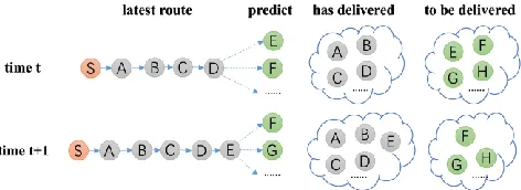
Figure 1: The delivery times of all packages at any time are af-fected by the latest route, the delivered pattern and the
to-be-delivered pattern.
such as the Cainiao Ltd., the traditional package delivery process is digitized and massive amount of delivery data are collected. The problem of how to precisely predict the ETA of packages has gained increasing attention in logis-tics research communities.
In the real scene, each courier should deliver nearly 100 packages per day. When customers demand, the delivery time of all undelivered packages should be predicted at the same time, which is a multi-destination prediction prob-lem. However, the problem can be referred from similar scenes, such as the car sharing and the free rider problem, where the travel time on the road and the sequence of the route are important. There exists valuable researches that can be referred, such as predicting the next location (Feng et al. 2018), mining delivery pattern (Ying, Lee, and Tseng 2013), and estimating time on the road (Jindal et al. 2018). Furthermore, the ETA of package delivery should consider both spatial and temporal features of the delivery route and researches can be found that propose spatial-temporal models in solving similar problems (Liang et al. 2018). However, predicting the package delivering time is chal-lenging mainly of the following reasons:
Multiple destinations. Predicting the travel time in trans-portation problem focuses on the time difference between an origin and a destination. However, in delivery system all undelivered packages should be predicted at any time. The delivery time of different locations may vary due to the delivery sequence and the locations of the packages.
Time-variant delivery status. As shown in Figure 1, the delivery time is affected by many factors especially the sequence of the latest route, the regularity of the delivery pattern and the sequence of packages to be delivered, which are difficult to learn by traditional model. Though recurrent neural networks (RNN) can learn sequential fea-tures, it could not handle frequent patterns and regularities of delivery routes.
Time-invariant delivery features. The geographical loca-tions of the packages have huge influence on the delivery sequence and thus determine the delivery time. The repre-sentation of the location in the model becomes an im-portant issue. Furthermore, the inherent properties of pack-ages such as the weight or size of the package should be considered.
To overcome the aforementioned difficulties, this paper proposed a novel wide and deep neural network for esti-mating time of package arrival (DeepETA). DeepETA has specially designed architecture to handle all the relative features of package delivery. The main contributions are as follows:
We develop a spatial-temporal module to capture the se-quential features of the latest delivery route. Different from traditional methods that use one-hot or convolution layer to represent geo-locations, we first encode the location ac-cording to the geographical proximity and then embed them into short vectors. Combining with delivering status of each node in the delivery route, the long short-term memory cells (LSTM) are used to extract the sequential features of the route.
We design two attention-based modules to learn histori-cal frequent and relative delivery patterns. To tackle the difficulty that RNN cannot learn the correlations between massive historical data, we first extract relative delivery routes and utilize attention mechanism to find the most similar route. Both delivered and undelivered packages are taken into account to enrich the model.
We evaluate the proposed method on a real-world logis-tics dataset. The results show that our approach outper-forms the competing methods.
Related Work
The problem of predicting the delivery time of multiple destinations can be referred from predicting the next loca-tion, estimating the travel time of vehicles on the road, and spatial-temporal model used for time series prediction.
Next location prediction: (Ying, Lee, and Tseng 2013) builds the frequent pattern tree and utilizes traditional machine learning methods to predict the next location. (Wu et al. 2017) proposes an LSTM network that can learn the path sequential features. (Zhang et al. 2018) predicts taxi destination by transforming raw trajectories into image and used convolutional neural network (CNN) to extract deep spatial features. RNN is used to model temporal and sequential features. (Feng et al. 2018) develops an attentional recurrent model considering both heterogeneous transition regularity and multi-level periodicity. If the next location is precisely predicted, the travel time can be simply calculated by the distance and velocity.
Estimating travel time: (Wang, Fu and Ye 2018) uses ensemble model that combines linear models, deep neural network (DNN) and RNN. (Jindal et al. 2018) proposes two DNN modules to capture coordinates and time attrib-utes from raw trajectories. (Zhang et al. 2018) develops a bi-directional LSTM layer to capture short-term and long-term traffic features. (Li et al. 2018) utilizes multi-task learning to predict the additional feature of the path and jointly learn the main task. (Wang et al. 2018) designs an end-to-end network that contains a geo-convolution layer to represent raw trajectory and used multi-task to learn both the entire path and each local path.
Spatial-temporal data prediction: Delivery time predic-tion is a time-series problem and methods in similar fields can be inferred. (Shen et al. 2018) treats the time series data as video and proposed a CNN to simultaneously mod-el all corrmod-elated spatial-temporal mobility patterns. (Liang et al. 2018) proposes a multi-level attention networks for geo-sensory time series prediction and utilizes spatial at-tention to capture the geographical correlations. (Yao et al. 2018) uses geo-convolutional layer to model spatial rela-tions and LSTM to model the time series. (Zhang et al. 2018) extracts distant, near and recent flows manually to model temporal features and uses residual networks to bet-ter train the deep networks. (Yao et al. 2018) utilizes the attention mechanism to find the periodicity and temporal shifting.
Preliminaries
In this section, the delivery time prediction problem is de-fined and related notations are explained.
problem. We utilize an optimized partition method based on road network and areas of interest (AOI). The partition function of mapping package 𝑝𝑖 to location 𝑎𝑖 is defined as 𝑎𝑖= 𝑂(𝑝𝑖).
Delivery route: After the aggregation step, the task is transformed to predict the deliver time of a set of locations, namely 𝑆𝑒𝑡 = {𝑎𝑖 | 𝑖 = 0, ⋯ , 𝑛}. The sequence of locations has great impact on the delivery time. We define the deliv-ery sequence at time 𝑡𝑖 in day 𝑑 as:
𝑡𝑒 , = {𝑛 𝑑𝑒 , 𝑛 𝑑𝑒 , ⋯ 𝑛 𝑑𝑒 , }, (1) where 𝑛 𝑑𝑒 , is a spatial-temporal node that means loca-tion 𝑎𝑐 is visited at time 𝑡𝑖.
Problem definition: The delivery time 𝑑𝑡𝑖 of location 𝑎𝑖 is the travel time from the current location 𝑎𝑐 to destination 𝑎𝑖. The sequence of the current route and the undelivered location set have great influence on the delivery time. We develop a deep learning method to learn the regularity from massive historical data. First, given the latest route 𝑡𝑒 , and the predicted location 𝑎𝑖, we find all rela-tive routes from history that are similar with the current route, symbolized as set ℋ𝑟𝑜𝑢 𝑒. Then, given the undeliv-ered location set 𝑆𝑒𝑡 ,, we find all routes from history that has similar undelivered set, marked as ℱ𝑠𝑒 . All records have a delivery time of 𝑎𝑖. The objective of our network is to find the most possible delivery time 𝑑𝑡 from historical relative routes:
𝑑𝑡 = (ℋ𝑟𝑜𝑢 𝑒, ℱ𝑠𝑒 ) (2)
Proposed DeepETA Framework
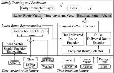
In this section, the proposed spatial-temporal sequential network for estimating time of package arrival (DeepETA) is described in detail. Figure 2 shows the architecture of the proposed method. The DeepETA is an end-to-end net-work that takes variant route feature and time-invariant feature as input, and output the delivery time. DeepETA consists of three modules, namely the latest route encoder, the
frequent pattern encoder, and the prediction module.
Latest Route Encoder
This module aims to capture the complicated sequential information that influences the delivery time. The delivery route is consecutive in time and is adjacent in space. Previ-ous location prediction literatures, such as (Monreale et al. 2009; and Ying et al. 2013), claim that human mobility can be regarded as a probability chain. The future locations or behaviors can be predicted through the transition probabil-ity matrix given the past behaviors. Hidden Markov Model (HMM) are used to model the process. However, HMM suffers from the deficiency of learning long-term
depend-encies. Recently, RNN has gained a breakthrough in se-quential mining. (Mikolov et al. 2010) develops RNNs in word embedding for sentence modeling. Multiple hidden layers in RNN
Figure 2: The framework of the proposed DeepETA. The model inputs consist of time-variant route features and time-invariant features and the output 𝑦𝑖 is the delivery time of package 𝑎
𝑖 at
time 𝑡.
can adjust dynamically with the input of behavioral history and the transition probabilities can be transmitted through the whole sequence. In this paper, the LSTM cells (Hochreiter and Schmidhuber 1997) are used to overcome the gradient vanishing or exploding problem of RNN. In delivery problem, locations are also important as the geo-graphical distance decides the sequence of delivery. We develop a spatial encoder to vectorize the locations. Spatial encoder: Locations in the delivery route have spatial correlations. Traditional methods use one-hot en-coder to represent locations and manually extract the spa-tial features, which may lose the information of distant areas. Recently, DNN and CNN are widely used (Zhang et al. 2018; and Shen et al. 2018) because they can automati-cally extract the spatial relation. However, CNN needs to split the space into grids with the same height and width, which may cause the uncertainty granularity problem. If the size is too big, we cannot distinguish different ETAs in that large area. If it is too small, neighborhood may be di-vided into several grids and regularity in same area may be lost. In this paper, we proposed a geocoding-based encoder to represent locations by their inherent geographical attrib-utes.
can be utilized by the neural networks. First, location 𝑎𝑖 is transformed into Geohash encoding of 40 digits, namely 𝐺 . Then an embedded layer is added to represent 𝐺 aim-ing at reducaim-ing computation cost without losaim-ing much in-formation, formulated as:
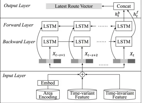
Figure 3: The structure of the Latest Route Representation layer. The locations are encoded by the spatial encoder. Then features of each node in the delivery route are exported to a bidirectional LSTM layer. The outputs of the last cell of the backward layer ℎ𝑏
and the forward layer ℎ𝑓 are combined to form the latest route vector.
= ( 𝐺 ), (3)
where and are learnable parameters of the spatial embedding layer and the Relu activation function is uti-lized to add non-linearity.
BiLSTM: The LSTM cell is able to capture the temporal sequential dependency, which improves the weakness of gradient exploding and vanishing of traditional RNN. As compared with LSTM, bidirectional LSTM (BiLSTM) (Graves and Schmidhuber 2005) utilizes additional back-ward information and thus enhances the memory capabil-ity. In the latest route representation layer, we use BiLSTM to capture the transition probability of each node in the route and to infer delivery time by the hidden state vector of the last cell.
We concatenate the vectors of the spatial encoder , with time-variant features 𝑣 and time-invariant features 𝑖 to get the global feature vector 𝑋 of each timestep, i.e., 𝑋 = [ , 𝑣, 𝑖]. A set of 𝑋 contained fixed length of time steps is fed into the BiLSTM layer. LSTM utilizes two gates to control the cell state. The forget gate decides how much information of the last cell state 𝑐 −1 will keep to the current time 𝑐 . The other is the input gate, which decides how much information of the input of the current networks 𝑋 will keep to cell state 𝑐 . LSTM uses the out-put gate to control how much information of the cell state
𝑐 will output to ℎ . Thus the conveyor belt-like structure allows LSTM to remove or add information from the very beginning to the current state. Then we get the latest hid-den states ℎ𝑏 and ℎ𝑓 of the forward and backward layer. Each of them can be calculated by ℎ = 𝐿𝑆𝑇𝑀(ℎ −1, 𝑋). Finally, these two states are concatenated to get the hidden state of the latest route ℎ = [ℎ𝑏, ℎ𝑓].
Frequent Pattern Encoder
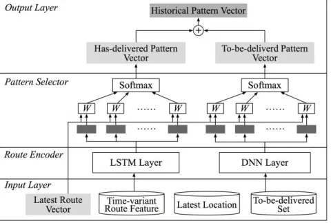
The frequent pattern encoder is designed to capture the frequent mobility patterns by jointly selecting the most related historical delivery routes under the current delivery status. The module consists of two parts. The route encoder first extracts spatial-temporal features from the historical delivery routes. Then these features are selected by an at-tention-based layer based on the latest route vector to gen-erate the most related pattern. By combining this vector with the latest route, we could predict the delivery time based on not only the sequential relation but also the fre-quent pattern of the historical routes.
Route encoder: Although the LSTM cell improves the problem of gradient exploding and vanishing, the perfor-mance of LSTM drops significantly when the length of time step is very long (Bengio, Simard, and Frasconi 1994). Simply importing all historical routes into the recur-rent layer may reduce the effectiveness and increase train-ing difficulty. In neural machine translation, it suffers from similar problem that RNN cannot memorize long sentenc-es. (Bahdanau, Cho, and Bengio 2014) develops the atten-tion mechanism which can selectively maintain infor-mation about the most relative word. Furthermore, atten-tion is widely used in object recogniatten-tion (Xu et al. 2015) to recognize the most interested area from the whole image. Different from the attention mechanism, which requires the whole sentences, we design a route selector that ex-tracts only the relative frequent patterns. Assuming that the latest route at time 𝑡𝑖 is 𝑡𝑒 , and the undelivered location set is 𝑆𝑒𝑡 , , we separately select the frequent patterns by the following rules:
Delivered route pattern: Given the current location 𝑎𝑖, the travel time of the latest delivery route 𝑡𝑖 and the pre-dicted location 𝑎𝑖, we find historical delivery routes that have the same current location and travel time, which will significantly reduce the scale of the candidates. Then we group these routes by the discrete delivery time bin (30 min) of 𝑎𝑖 and find the top 10 most regular routes for each time bin, defined as ℋ𝑟𝑜𝑢 𝑒 in Eq. (2). The task is to find which historical route is the most similar to the current route. So we utilized LSTM cells to represent the frequent routes:
where k is the class of delivery time. ℋ̃tk is the context vector of all frequent routes that has 𝑘 delivery time and we compute the average value of all vectors in each time bin. Furthermore, statistic features such as the frequency of each time bin are concatenated with the context vector.
To-be-delivered pattern: Different from the delivered route, the exact delivery order is unknown. So we use the
Figure 4: The architecture of the frequent pattern encoder. This module has the same input with the network and is connected to the latest route module. The output is the representation of
histor-ical relative pattern.
current location 𝑎𝑐, the number of locations in the delivery set 𝑛𝑖 and the predicted location 𝑎𝑖 to find historical to-be-delivered sets. Similar with the above step, we group these sets by the same time bin as the delivered pattern module and 10 frequent sets are selected in each time bin, marked as ℱset. As the sequence of the current to-be-delivered lo-cations is hard to predict, it is not proper to use sequential layer like LSTM. Instead, a DNN is developed to model the unordered set and reduce the impact from sequences:
ℱ̃ = (ℱ̃ −1, ℱ𝑠𝑒 ), (5)
Pattern selector: The goal of the pattern selector is to find which frequent pattern has the biggest impact on the current situation. Traditional pattern mining methods uti-lize similarity measurements such as the cosine similarity, Levenshtein distance, and the time dynamic wrapping. However, pattern mining methods may suffer from data sparseness problem and complex features cannot be weighted. An attention-based layer is designed to calculate the similarity between the latest route and the frequent routes. First, the frequent pattern vectors are combined with the latest route vector through a score function:
(ℋ̃ , ℎ) = 𝑡𝑎𝑛ℎ(ℋ̃ 𝑠𝑐𝑜𝑟𝑒ℎ ), (6)
where ℋ̃ or ℱ̃ is the frequent pattern vectors, 𝑠𝑐𝑜𝑟𝑒 is a learnable parameter, and ℎ is the latest route vector. Then
all scored vectors are exported to the softmax layer to cal-culate the weight of each vector. The softmax is the exten-sion of the sigmoid function to the multi-class problem, which transforms the 𝐾 dimension variable into another 𝐾 dimension variable within (0,1):
( ) =∑𝑒 𝑒
, (7)
where = (ℋ̃ , ℎ) and 𝐾 is the total number of the de-livery time bins. Finally, the value of the softmax is multi-ply with the historical pattern vectors that can illustrate the importance of different patterns:
𝑓 = ∑( ( ) ℋ̃ ), (8)
Jointly Training and Prediction
The predicted delivery time of location 𝑎𝑖 at time 𝑡 is relative with the properties of packages in 𝑎𝑖, the latest route features and the frequent patterns. We concatenate the outputs from the latest route module ℎ and the fre-quent pattern encoder 𝑓 , together with the time-invariant features 𝑖:
𝑋̃ = [ℎ, 𝑓 , 𝑖], (9)
Then 𝑋̃ is fed into a fully connected layer to get the final prediction value 𝑦̃ :
𝑦̃ = ( 𝑓𝑐𝑋̃ 𝑓𝑐), (10) where 𝑓𝑐 and 𝑓𝑐 are learnable parameters and (𝑥) is the activation function of the last fully connected layer. The Sigmoid function defined as (𝑥) = 1/(1 𝑒−𝑥) is used to restrict the output in [0,1], as the prediction values are normalized.
The loss function consists of two parts: the mean square error (MSE) and the mean absolute percentage square error (MAPSE). MSE is like a combination measurement of bias and variance of the prediction but is sensitive to large pre-diction values. However, in delivery task, there might be some cases that the customer is not at home and requires a second delivery which leads to large ETA. MAPSE gives less weight to outliers, which is not sensitive to outliers. So we decide to combine the advantages of MSE and MAPSE to make the prediction mainly focus on normal and small ETA to reducing the influence of outliers. There exists a jointly training trick by adding a hyper parameter to adjust the weight of MSE and MAPSE. The loss function is de-fined as follows:
( ) = ∑𝑖 1((𝑦̃ 𝑦) ( ̃− ) ), (11)
net-work that can be trained in the whole netnet-work. During the training phase, the Adam optimizer (Kingma and Ba 2014) is used to minimize the loss function.
Experiments
Dataset Description
The experiment is conducted on a real-world package de-livery dataset collected by Cainiao Ltd., which is one of the largest logistics companies in China, handling over a hun-dred million packages per day. The dataset contains the delivery routes of 331 couriers from Jun. 1, 2018 to Aug. 1, 2018 (60 days), in Beijing, China. As shown in Table 1, each courier delivers 80 packages in 2 delivery routes eve-ry day and the average working time is 8 hours. The aver-age delivery time of all the packaver-ages is 3.5 hours. The av-erage number of nodes in each delivery route is 20. Each sample of the dataset contains the static properties of pack-ages, such as the location, weight, date, holiday and courier ID. Also the time-variant features, such as the latest route info. Each node in the route consists of the current loca-tion, time, distance to the prediction location and delivery status. In total there are 350 thousand samples to be pre-dicted. The previous 50 days are used as training set and the last 10 days as testing set.
Evaluation Metric
Mean Average Percentage Error (MAPE) and Rooted Mean Square Error (RMSE) are used to evaluate the proposed methods. MAPE can intuitively show the deviation be-tween the prediction and the ground truth, and RMSE is the absolute value to show the performance of the model. Both of them are widely used in time series prediction problem, which are defined as follows:
𝑀 =1∑ |𝑦̂𝑡−𝑦𝑡|
𝑦𝑡
𝑖 1 , (12)
𝑀𝑆 = √1∑𝑖 1(𝑦̂𝑡 𝑦𝑡) , (13)
where 𝑦̂ and 𝑦 are the prediction and the ground truth of the deliver time of location 𝑎 at time 𝑡, and is the total number of samples.
Methods for Comparison
The proposed methods are compared with the following methods:
Linear regression (LR): We use Lasso (i.e., with ℓ1 -norm regularization) as the linear regression method.
XGBoost (Chen and Guestrin 2016): XGBoost is widely used in many machine learning problems and data science challenges and it always surpasses other traditional models.
A common trick on utilizing traditional model in sequential data is to unfold the time series and concatenate each time step together.
Deep neural network (DNN): A neural network of four fully connected layers to extract the high level correlation
Table 1. Statistics of the delivery status of each courier per day.
Pkgs Route Nodes Time AvgDt
80 2 20 8h 3.5h
between the combining vectors. The number of hidden units are 128, 128, 64, and 32 respectively.
LSTM: A stacked LSTM network to model sequential route features. The hidden units are 64 and 64.
DeepTTE (Wang et al. 2018): A state-of-art network in travel time prediction which utilizes geo-convolutional layer to represent raw trajectories and uses a combination of the LSTM cell and attention mechanism to learn long-term dependency of one route. We replace the convolution layer with our location vector and uses the default settings in the open source code.
DeepMove (Feng et al. 2018): A state-of-art method in next destination prediction that has a recurrent layer to model current movement and uses attention mechanism to learn historical patterns. We modify the output softmax layer to a fully connected layer to make regression.
Furthermore, the effects of different modules in Deep-ETA are evaluated.
Latest route representation (BiLSTM): Only the latest route module is reserved to see the effectiveness of model-ing sequential route through the BiLSTM.
Frequent pattern encoder (BiLSTM+DP and BiLSTM +TP): In the frequent pattern encoder, both historical deliv-ered patterns and to-be-delivdeliv-ered patterns that matter. First, only the delivered patterns are remained. Then we adapt the to-be-delivered patterns individually.
Preprocessing and Parameters
has 64 and 32 units. We further conduct experiment to ad-just the hyper-parameter in the loss functions: only RMSE, only MAPE and the combination. The experiment shows that the mix loss function reduces 10.8% error compared to single metrics.
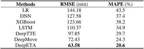
Table 2. The performance of different baselines and DeepETA.
Methods RMSE (min) MAPE (%)
LR 144.18 43.5
DNN 127.58 37.4
XGBoost 123.66 38.2
LSTM 110.37 34.9
DeepTTE 97.85 29.7
DeepMove 72.43 24.3
DeepETA 63.58 20.6
Model Comparison
Table 2 shows the performance of the proposed method compared to the baseline models. DeepETA achieves the lowest RMSE (63.58 minutes) and the lowest MAPE which improves the best performance of the baseline methods by 13.8% (RMSE) and 16.5% (MAPE). The Las-so based linear regression performs poorly because it only utilizes the properties of time series and could not learn neither short-term or long-term dependencies. Regression methods such as DNN and XGBoost unfold sequential data into unordered vectors and can learn the co-occurrence of each time step, which achieve better performance. Simple LSTM network can extract the correlations from the be-ginning of the route to the end. However, it suffers the long-term dependency problem when dealing long se-quence. DeepTTE gains better performance than LSTM (11.8% improvement of RMSE) because it uses attention mechanism to enhance the ability of learning long se-quences. Traditional methods only focus on modeling each route while DeepMove is designed to utilized historical frequent mobility, which lead to a significantly enhance (25.5% improvement of RMSE than DeepTTE). Our method DeepETA gains an improvement of 13.8% in RMSE than DeepMove. The main difference is that in the attention layer, DeepMove uses sampling method to extract high level features to represent historical trajectories and we develop a LSTM-based layer to extract the sequential features from raw routes. Meanwhile, we are more con-cerned about the sequence of the undelivered set and spe-cially design a DNN layer to focus on these features.
Effectiveness of model components
The latest route representation layer of DeepETA aims to extract sequential relations of the current route by BiLSTM cells. Purely rely on this layer, the performance outper-forms the LSTM cell slightly (an improving of 6%). As shown in Figure 5a, when adding the frequent pattern
en-coder, the performance significantly increases. The deliv-ered pattern encoder improves the RMSE by 36.5% com-pared to BiLSTM only. The to-be-delivered pattern encod-er has an improvement of 29.8% and the combination of all modules improves the overall performance by 3%, which makes the DeepETA to achieve the best score among base-line models.
(a) (b)
Figure 5: (a) The effectiveness of the components of DeepETA. (b) The performance of predictions at different time.
The differences between the latest route and the frequent pattern encoders is that if we just put all historical routes into the model without any frequent patterns selected ahead, the results are poorly. The reason is that the LSTM-based module may not memory the regularity among all historical routes and similar patterns may be lost. Deliv-ered route and undelivDeliv-ered pattern are treated separately as we do not know the delivery sequence of undelivered packages and sequential features should not be considered in modeling undelivered pattern. As a result, we have two probability distributions drew differently from delivered and undelivered patterns.
Performance of prediction at different time
Conclusion
In this paper, we propose a deep spatial-temporal sequen-tial model for estimating the package delivery time (Deep-ETA). First, the latest route encoder embeds the location of packages that remain geographical relations and BiLSTM is used to model the sequential features. Then, the frequent pattern encoder selects the frequent routes from historical data and uses LSTM and DNN to represent the routes. An attention-based layer is developed to calculated the most similar patterns with the current route. Finally, by combin-ing all these features, jointly traincombin-ing is utilized to mini-mize the loss function. Experiments on real logistics da-taset show that the proposed method overwhelms the start-of-art methods and the effectiveness of three modules are illustrated.
In the future, we will extend our work in the following aspects. First, we use the unordered undelivered set as the sequence of the route is unknown. If the sequence of the route can be precisely predicted, the delivery time is easy to be inferred. Then, we predict the to-be-delivered pack-ages at time 𝑡 separately. Inspire by the real-time neural machine translation and the sequence to sequence model, the model can predict the following multiple time steps at once without losing accuracy.
References
Abadi, M.; Barham, P.; Chen, J.; Chen, Z.; Davis, A.; Dean, J.; ... and Kudlur, M. 2016. Tensorflow: a system for large-scale ma-chine learning. In Proceedings of the 12th Symposium on Operat-ing Systems Design and Implementation, 265-283.
Bahdanau, D.; Cho, K.; and Bengio, Y. 2014. Neural machine translation by jointly learning to align and translate. arXiv pre-print arXiv:1409.0473.
Bengio, Y.; Simard, P.; and Frasconi, P. 1994. Learning long-term dependencies with gradient descent is difficult. IEEE transactions on neural networks, 5(2): 157-166.
Chen, T., and Guestrin, C. 2016. Xgboost: A scalable tree boost-ing system. In Proceedings of the 22nd ACM SIGKDD interna-tional conference on knowledge discovery and data mining, 785-794. ACM.
Feng, J.; Li, Y.; Zhang, C.; Sun, F.; Meng, F.; Guo, A.; and Jin, D. 2018. DeepMove: Predicting Human Mobility with Attentional Recurrent Networks. In Proceedings of the 2018 World Wide Web Conference on World Wide Web, 1459-1468.
Graves, A., and Schmidhuber, J. 2005. Framewise phoneme clas-sification with bidirectional LSTM and other neural network ar-chitectures. Neural Networks, 18(5): 602-610.
Hochreiter, S., and Schmidhuber, J. 1997. Long short-term memory. Neural computation, 9(8): 1735-1780.
Jindal, I.; Chen, X.; Nokleby, M.; and Ye, J. 2017. A Unified Neu-ral Network Approach for Estimating Travel Time and Distance for a Taxi Trip. arXiv preprint arXiv:1710.04350.
Kingma, D. P., and Ba, J. 2014. Adam: A method for stochastic optimization. arXiv preprint arXiv:1412.6980.
Liang, Y.; Ke, S.; Zhang, J.; Yi, X.; and Zheng, Y. 2018. Geo-MAN: Multi-level Attention Networks for Geo-sensory Time Series Prediction. In Proceedings of the 27th International Joint Conferences on Artificial Intelligence, 3428-3434.
Li, Y.; Fu, K.; Wang, Z.; Shahabi, C.; Ye, J.; and Liu, Y. 2018. Multi-task representation learning for travel time estimation. In Proceedings of the 24th International Conference on Knowledge Discovery and Data Mining, 1695-1704.
Mikolov, T.; Karafiát, M.; Burget, L.; Cernocký, J.; and Khudan-pur, S. 2010. Recurrent neural network based language model. In Proceedings of the Eleventh Conference of the International Speech Communication Association, 1045–1048.
Monreale, A.; Pinelli, F.; Trasarti, R.; and Giannotti, F. 2009. Wherenext: A location predictor on trajectory pattern mining. In Proceedings of the 15th ACM SIGKDD International Conference on Knowledge Discovery and Data Mining, 637–646. ACM. Shen, B.; Liang, X.; Ouyang, Y.; Liu, M.; Zheng, W.; and Carley, K. 2018. StepDeep: A Novel Spatial-temporal Mobility Event Prediction Framework based on Deep Neural Network. In Pro-ceedings of the 24th ACM SIGKDD International Conference on Knowledge Discovery & Data Mining, 724-733. ACM.
Wang, D.; Zhang, J.; Cao, W.; Li, J.; and Zheng, Y. 2018. When Will You Arrive? Estimating Travel Time Based on Deep Neural Networks. In Proceedings of the Thirty-Second AAAI Conference on Artificial Intelligence.
Wang, Z.; Fu, K.; and Ye, J. 2018. Learning to Estimate the Trav-el Time. In Proceedings of the 24th ACM SIGKDD International Conference on Knowledge Discovery & Data Mining, 858-866. ACM.
Wu, F.; Fu, K.; Wang, Y.; Xiao, Z.; and Fu, X. 2017. A Spatial-Temporal-Semantic Neural Network Algorithm for Location Pre-diction on Moving Objects. Algorithms, 10(2): 37.
Xu, K.; Ba, J.; Kiros, R.; Cho, K.; Courville, A.; Salakhudinov, R.; ... and Bengio, Y. 2015. Show, attend and tell: Neural image caption generation with visual attention. In International confer-ence on machine learning, 2048-2057.
Yao, H.; Tang, X.; Wei, H.; Zheng, G.; Yu, Y.; and Li, Z. 2018. Modeling Spatial-Temporal Dynamics for Traffic Prediction. arXiv preprint arXiv:1803.01254.
Yao, H.; Wu, F.; Ke, J.; Tang, X.; Jia, Y.; Lu, S.; ... and Ye, J. 2018. Deep multi-view spatial-temporal network for taxi demand prediction. In Proceedings of the Thirty-Second AAAI Conference on Artificial Intelligence.
Ying, J.; Lee, W.; and Tseng, V. 2013. Mining geographic-temporal-semantic patterns in trajectories for location prediction. ACM Transactions on Intelligent Systems and Technology, 5(1): 2. ACM.
Zhang, H.; Wu, H.; Sun, W.; and Zheng, B. 2018. DeepTravel: a Neural Network Based Travel Time Estimation Model with Aux-iliary Supervision. arXiv preprint arXiv:1802.02147.
Zhang, J.; Zheng, Y.; Qi, D.; Li, R.; Yi, X.; and Li, T. 2018. Pre-dicting citywide crowd flows using deep spatio-temporal residual networks. Artificial Intelligence, 259: 147-166.