R E S E A R C H A R T I C L E
Open Access
Extended modelling of dislocation
transport-formulation and finite element
implementation
Michael M. W. Dogge
1,2, Ron H. J. Peerlings
2*and Marc G. D. Geers
2*Correspondence:
[email protected] 2Department of Mechanical Engineering, Eindhoven University of Technology, P.O. Box 513, 5600 MB Eindhoven, The Netherlands Full list of author information is available at the end of the article
Abstract
In the past decade, several higher-order crystal plasticity models have been developed to properly capture size effects, dislocation pile-up and patterning. Here we consider a formulation which accounts for the presence and behavior of both positive and negative dislocations in terms of densities. We derive an implicit finite element implementation for the continuum crystal plasticity model including dislocation transport, using a generalised continuum expression for the short-range dislocation interactions, by discretizing the two governing non-linear transport equations in time and space. The resulting non-linear algebraic equations are solved by an
incremental-iterative solution scheme. We compare the resulting numerical solutions with discrete dislocation simulations. This analysis shows the capabilities of the implicit FEM framework to solve continuum dislocation transport in crystal plasticity with the added energetic dislocation interactions.
Keywords: Finite element method, Crystal plasticity, Dislocation transport
Background
Crystal plasticity models are nowadays employed in a wide range of engineering applica-tions, and the finite element method is commonly adopted in numerical models employing them [1]. In particular, they allow one to study the effect of microstructural morphology of poly-crystalline materials. Relevant mechanisms such as anisotropy and plastic defor-mation along discrete slip planes, as found in crystalline materials, are captured in a natural fashion. However, other mechanisms such as size effects cannot be described by classical crystal plasticity [2,3]. Therefore, much attention has recently been given to the incorporation of strain gradient effects in crystal plasticity models.
Physically, the plastic slip on glide planes is the result of the collective motion of disloca-tions [4]. On a continuum scale many higher-order phenomenological models exist which capture, rather than describe, the behaviour of a large collection of dislocations. The work of Nye [5] provided a basis for such continuum models by introducing a dislocation density tensor, representing the accumulation of dislocations when non-homogeneous deforma-tion results in lattice incompatibility. The nodeforma-tion of Geometrically Necessary Dislocadeforma-tions (GNDs) was used to relate spatial gradients of strain to the presence of dislocations [6]. GNDs, emanating from strain gradients, can be used in a phenomenological way to e.g.
©2015 Dogge et al. This article is distributed under the terms of the Creative Commons Attribution 4.0 International License (http:// creativecommons.org/licenses/by/4.0/), which permits unrestricted use, distribution, and reproduction in any medium, provided you give appropriate credit to the original author(s) and the source, provide a link to the Creative Commons license, and indicate if changes were made.
elevate the strengthening of a slip system [7] or to increase the free energy of a system [8,9], leading to additional balance equations for the plastic slip. Based on these theories, numerical models were developed including the effect of dislocations on the plastic behav-iour of the material, either as strain gradients [10–12] or as additional degrees-of-freedom [13].
Here, we consider another class of higher-order crystal plasticity models, in which the presence and transport of dislocations is included more directly via dislocation densities. A crucial element in such models is the way they account for short-range dislocation interactions [14]. Such models may for instance be formulated using statistical mechanics arguments [15]. Here, however, we demonstrate that if the short-range interaction term is derived from an idealised dislocation configuration, it takes a slightly more general form, which apart from the usual gradient of GND density also contains a gradient of the total dislocation density. By upscaling the dislocation interactions in this idealized configuration we include all dislocation interactions in the continuum expression for the short-range stresses. This expression is used in the governing equations for the transport of dislocation densities, as adopted from models taking into account the evolution of dislocation densities [15–17].
The resulting initial boundary value problem contains two non-linear, coupled PDEs. In order to solve these equations numerically, they are discretised in space using the finite element method. In [16] the semi-discrete transport equations are solved using an explicit temporal discretisation. This however introduces the constraint of small time-steps in order to have stable numerical solutions.
A second objective of the present paper is therefore to formulate a fully implicit solution strategy, based on a backward Euler time integration. The obtained non-linear algebraic equations are then linearised and solved using a Newton-Raphson procedure. The evo-lution of the dislocation transport is thus simulated by an incremental-iterative scheme. Results obtained with this implementation are compared to discrete dislocation calcula-tions in order to study its validity.
Governing equations for the transport of dislocation densities Governing equations
In a crystal plasticity framework the plastic deformation is the result of plastic slip on distinct glide planes, and depends on the amount and orientation of such (active) slip systems. Using a small deformation assumption, for a single glide plane the total shear deformationγ can be expressed as:
γ =γe+γp. (1)
Here,γeandγprepresent the elastic and plastic deformation respectively. The stress due to this deformation is a result of the elastic deformation only. Adopting Hooke’s law the following relation for the elastic deformation is obtained:
γe= τ
G, (2)
whereτis the shear stress acting on a glide plane andGthe shear modulus. The framework is complete when an expression for the plastic slipγp is formulated. The choice forγp here is derived from the Orowan relation [4], which states that the plastic slip rate ˙γpis determined by the flux of dislocations:
˙
Here,bis the length of the Burgers vector andis the dislocation flux. An appropriate expression is required for the dislocation transport on a glide plane accompanying the dislocation flux.
Dislocation balance equations
In a continuum framework one refrains from keeping track of all individual dislocations and their positions. Instead, we describe the dislocations in terms of densities. We first choose to describe a collection of positive and negative infinite straight edge dislocations by positive densities ρ+(x, t),ρ−(x, t), where x is the coordinate along the slip system andtindicates time. Uniformity is assumed in all directions perpendicular to thex-axis, so that a one-dimensional problem remains. The resulting equations are subsequently reformulated in terms of the total and GND densitiesρ(x, t) andκ(x, t).
We consider the transport of a fixed number of positive and negative dislocations in a single slip system without creation and annihilation. The transport equations for the densities of positive and negative dislocations then read:
∂ρ+ ∂t +
∂+
∂x =0 (4)
∂ρ− ∂t +
∂−
∂x =0, (5)
where+and−are the fluxes of positive and negative dislocations, respectively, which still depend onρ+andρ−. To solve these transient PDEs we need initial and boundary conditions. The initial conditions are given by an initial density profile for both positive and negative densities, i.e.ρ+(x, t=0),ρ−(x, t=0). For an impenetrable barrier there can be no dislocation transport; therefore at such a boundary there is no flux:+=−=0. In the case of a free surface the dislocation densities vanish at this boundary.
The fluxes in (4) and (5) can be expressed as:
±=ρ±v±= ±bρ± B
τ+σint±, (6)
where the + sign holds for positive dislocations and the− sign for negative. For the velocity v±a linear drag law is adopted, such that the velocity depends linearly on the forces acting on the dislocations. Here,bis the length of the relevant Burgers vector, the sign depending on the sign of the dislocation,Bis the drag coefficient,τ the shear stress acting on the glide plane andσintis the short-range dislocation interaction stress.
The shear stressτ includes the stress due to the net incompatibility introduced by a large number of dislocations, as well as any externally applied loading. These stresses are naturally recovered in a crystal plasticity framework by the incompatibility of plastic deformation [5,18,19]. As the focus here lies on the transport of dislocations, we take
τ to be a constant, both in time and space. This is a valid assumption due to mechani-cal equilibrium in the material and for a stress-controlled deformation. The short-range interaction stress is the continuum equivalent of the interaction stresses between individ-ual dislocations. To close the PDEs (4) and (5), we still need to establish the dependence ofσshorton the dislocation densitiesρ+andρ−.
Upscaling of the short-range interaction stress
generalise the model by allowing for all dislocation gradients to contribute to the interac-tion stress. To formulate our continuum expression for the short-range internal stress we take into account the interactions between all dislocations as follows.
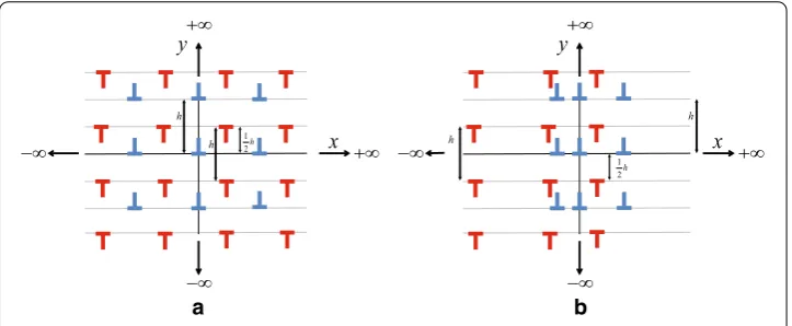
The starting point of the derivation is an idealized dislocation configuration of a single slip system in an infinite medium, containing infinite positive and negative dislocation walls with a constant vertical spacingh. The periodic dislocation wall (tilt wall) configu-ration studied here does not generate any long range stress, and is therefore suitable to characterise the short-range nature of the interaction stresses [14]. In this analysis we do not take into account dislocation sources and we avoid annihilation by assuming that no two dislocations of opposite sign exist on the same glide plane. However, the horizontal distribution of positive and negative walls can be arbitrary. Furthermore, we consider all walls to be mobile.
We consider the total interaction stress on both a positive and a negative wall. If there are many walls within a horizontal distance of±hfrom a particular wall, i.e. the horizontal distance between walls is much smaller than the vertical spacinghwithin the wall, we can assume a continuous distribution of dislocation walls. Then, we can rewrite the discrete sum of individual interaction stresses in a continuum equivalent for the total interaction stresses on a positive and negative wall as follows:
σint±(x)=
∞
−∞hρ
+(x−ξ)σ±+(ξ)dξ+ ∞ −∞hρ
−(x−ξ)σ±−(ξ)dξ. (7)
In this expression,σ±+andσ±−are the interaction stresses acting on a positive or negative dislocation wall due to another, positive or negative wall respectively, at a distanceξto the left. The integral runs from−∞to∞, taking into account all interactions and assuming a continuous distribution of dislocations with infinitesimally small distances. The linear densitieshρ±are a measure for the local number of walls.
The shear stress of an infinite periodic wall of positive edge dislocations is given by [20]:
σ = πGb (1−ν)h
˜
x(cosh 2πx˜cos 2π˜y−1)
(cosh 2πx˜−cos 2πy˜)2 , (8)
a b
Fig. 1 Taylor lattice (a) and a general configuration (b) with infinite positive and negative dislocation walls. The negative walls are shiftedh/2 with respect to the positive walls
adjacent dislocations on the same glide plane are more likely to be also positive than nega-tive. It is worth pointing out that the correlation between dislocations—which admittedly may be partially exaggerated—also implies that the dislocation configuration surround-ing an arbitrary positive dislocation is different from that of a negative dislocation and different interaction forces may thus be experienced by them.
Using this configuration, we can derive from Eq. (8):
σ++ = −σ−−=σ(˜x,y˜=0)= πGb¯ h
˜ x
sinh2πx˜ (9)
σ+− = −σ−+=σ(˜x,y˜=1/2)= πGb¯ h
˜ x
cosh2π˜x, (10)
where ¯G=G/(2(1−ν)).
Furthermore, the dislocation density at position (x−ξ) is estimated by a first order Taylor approximation around pointxfor bothρ+andρ−:
ρ±(x−ξ)=ρ±(x)−ξ∂ρ±
∂x . (11)
If we substitute the expressions (9), (10) and (11) in Eq. (7) and compute the resulting integrals, we obtain expressions for the total interaction stresses acting on a positive and a negative dislocation which may be written as:
σint±(x)= ∓Gbh¯
2
6
2∂ρ
± ∂x +
∂ρ∓ ∂x
. (12)
Finally, if we substitute (12) in (6) we obtain the following expression for the dislocation fluxes:
±=ρ±±bτ
B −ρ
±Gb¯ 2h2
6B
2∂ρ
± ∂x +
∂ρ∓ ∂x
. (13)
Using (13) in (4) and (5) respectively, these PDEs are fully expressed in terms ofρ+(x, t) and
ρ−(x, t) and we can thus calculate the evolution of the positive and negative dislocation
densities.
Formulation in terms of total dislocation and GND densities
In order to more easily relate the dislocation densities to relevant and meaningful (macro-scopic) properties, e.g. incompatibility and hardening, we rewrite the dislocation densities in terms of the total dislocation density ρ, and the Geometrically Necessary Disloca-tion densityκ. The GNDs are dislocations which are required to conform to the overall deformation, i.e. they characterize the incompatibility introduced by plastic slip [5]. The remaining dislocations are called Statistically Stored Dislocations (SSDs); they do not have a net geometrical contribution. The total density then reads:
ρ=ρSSD+ |κ|. (14)
Because of this relation, we only need two quantities to describe the evolution of all dislocations. A convenient choice is the combination of ρ andκ, because they have a clearer physical meaning and they can be easily related to the densities of positive and negative dislocations:
ρ =ρ++ρ− (15)
κ =ρ+−ρ−. (16)
Using the above relations we can determine the transport equations forρandκby adding (5) to (4) and subtracting (5) from (4) respectively:
∂ρ ∂t +
∂κ
∂x =0 (17)
∂κ ∂t +
∂ρ
∂x =0, (18)
where κ = ++−andρ = +−−. The latter characterises the total flow of Burgers vector, irrespective of the sign of the dislocations which carry it, and thus the plastic slip rate. The former gives the net flow of Burgers vector. Using (15) and (16) and the fluxes for positive and negative dislocations (13), the fluxesρ andρ can be expressed in terms ofρandκas:
κ = bτ Bκ−
¯ Gb2h2
12B
3ρ∂ρ
∂x +κ
∂κ ∂x
(19)
ρ = bτ Bρ−
¯ Gb2h2
12B
ρ∂κ∂
x +3κ
∂ρ ∂x
. (20)
Eqs. (17)–(20) are a closed set of equations in terms ofρandκ.
Implementation
In the numerical implementation of our model we need to solve the transport equations (17) and (18) for the total dislocation and GND densities. Although these equations are of a convection-diffusion nature, no stabilization is applied here. Most stabilization techniques use the addition of artificial diffusion. Here, the expression for the short-range dislocation interactions is of a diffusive nature. If one is to study these interactions in detail, addition of stabilizing diffusion can be of influence on the results. Therefore, no stabilization is introduced and care was taken choosing a sufficiently small element size and time step to ensure stability.
Time discretisation
First, the transient terms in the transport equations are discretised using a finite difference approach. For the temporal discretisation the implicit, backward Euler method is used:
ρ−ρ(t)
t +
∂κ
∂x =0 (21)
κ−κ(t)
t +
∂ρ
∂x =0. (22)
The symbols with superscript (t) represent the values at the previous time step. For brevity we dropped the superscript (t+t) for the values at the end of the current time step. This implicit time integration is used for additional stability and accuracy.
Spatial discretisation
For the spatial discretisation, the Galerkin method is adopted. By multiplying Eqs. (21) and (22) by test functionsψρ andψκ, and integrating the resulting expression over the domain (0, L) the weighted residuals formulation is obtained. Subsequently, integration by parts is applied, resulting in the weak forms:
L
0
ψρρ−ρ
(t)
t −
dψρ dx κ
dx+ψρκ L0=0 (23)
L
0
ψκκ−κ
(t)
t −
dψκ dx ρ
dx+ψκρ L0=0. (24)
The degrees-of-freedomρ,κand the test functionsψρ,ψκ are discretised using the same shape functionsN
∼(x): ρ =N∼Tρ∼, ψρ =ψ
∼ T
ρN∼ κ =N∼T∼κ, ψκ =ψ
∼ T
κ N∼.
Substituting these discretised variables in the weak forms (23) and (24) and requiring that they hold for allψ
∼ρandψ∼κ we obtain:
R
∼ρ =
L
0
⎛ ⎝N
∼
ρ−ρ(t)
t −
dN∼ dxκ
⎞ ⎠dx+ N
∼κ
L 0 =0 ∼ (25) R
∼κ =
L
0
⎛ ⎝N
∼
κ−κ(t)
t −
dN∼ dxρ
⎞ ⎠dx+N
∼ρ
L
0
=0
∼. (26)
Note that the dislocation densitiesρ,κand the fluxesρ,κ can be expressed in terms of the discretised valuesρ
Linearisation
The expressions (19) and (20) for the fluxes are non-linear; therefore an iterative solution strategy is used to solve equations (25) and (26). Here we use the Newton-Raphson method and we thus need to linearize the equations. This implies that we substitute forρandκ:
ρ =ρ(i)+δρ κ =κ(i)+δκ,
where (i) andδdenote the estimate obtained from the previous iteration and a variation (or iterative correction), respectively. The iterative updates for the fluxesδρandδκare obtained by linearising (19) and (20) with respect to the degrees-of-freedomρ,κ, giving:
δκ = bτ Bδκ−
¯ Gb2h2
12B
3∂ρ
(i)
∂x δρ+3ρ
(i)∂δρ ∂x +
∂κ(i) ∂x δκ+κ
(i)∂δκ ∂x
δρ = bτ Bδρ−
¯ Gb2h2
12B
∂κ(i) ∂x δρ+3κ
(i)∂δρ ∂x +3
∂ρ(i) ∂x δκ+ρ
(i)∂δκ ∂x
.
After discretisation and linearisation we obtain the following linear system of equations for the iterative corrections:
Kρρ Kρκ Kκρ Kκκ
⎡ ⎣δ ρ∼
δ κ ∼ ⎤ ⎦= − ⎡ ⎢ ⎣R∼
i
ρ
R
∼iκ
⎤ ⎥
⎦, (27)
with:
Kρρ =
L
0
⎛ ⎝ 1
tN∼N∼ T +dN∼
dx ¯ Gb2h2
4B
∂ρ(i) ∂x N∼
T+ dN∼
dx ¯ Gb2h2
4B ρ
(i)dN∼ T
dx
⎞ ⎠dx
Kρκ =
L
0
⎛ ⎝−dN∼
dx bτ
BN∼
Tdx+ dN∼
dx ¯ Gb2h2
12B
∂κ(i) ∂x N∼
T+ dN∼
dx ¯ Gb2h2
12B κ
(i)dN∼ T
dx
⎞ ⎠dx
Kκρ =
L
0
⎛ ⎝−dN∼
dx bτ
BN∼ T +dN∼
dx ¯ Gb2h2
12B
∂κ(i) ∂x N∼
T +dN∼
dx ¯ Gb2h2
4B κ
(i)dN∼ T
dx
⎞ ⎠dx
Kκκ =
L
0
⎛ ⎝ 1
tN∼N∼ T +dN∼
dx ¯ Gb2h2
4B
∂ρ(i) ∂x N∼
T+ dN∼
dx ¯ Gb2h2
12B ρ
(i)dN∼ T
dx
⎞ ⎠dx
When an appropriate numerical integration scheme, e.g. Gaussian integration, to approx-imate the above integrals is chosen, the residualsR
∼and the tangentsKcan be constructed
element-wise and assembled in order to solve Eq. (27). In this work, linear shape functions are chosen, and a two-point Gauss integration scheme.
Simulations and results
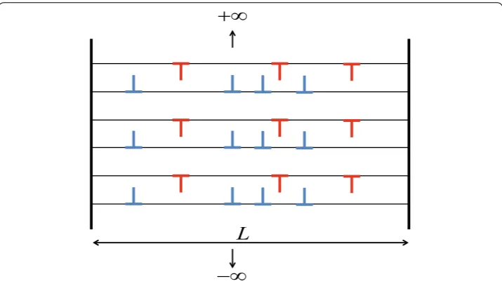
Fig. 2 Infinite vertical dislocation walls with both positive and negative signs in a domain with lengthL. The distribution of walls is determined by the density profile. The boundaries are either impenetrable or free. An external shear stress is applied
An external shear stressτ is applied to the system. This shear stress is considered to be constant along the slip system for both the continuum and the discrete framework, because of equilibrium and because the long-range stresses for infinite dislocation walls vanish. We can therefore focus on the transport of dislocations in single slip.
After rescaling the material parameters in the governing equations, the relevant para-meters are the ratiosb/h,L/handτ/G¯. In the simulations a fixed ratio ofb/h= 1/200 is used. The ratiosL/handτ/G¯ vary between the simulations. The number of finite ele-ments used is 200. For the choice of the time step size, first a characteristic time can be estimated using the dislocation velocity. This velocity is determined by the linear drag law, only using the applied stress. Using this relation an upper bound for the time step can be estimated, i.e.t≈hv−1≈B/(bτ). An appropriate time step size should be much
lower than this value to obtain accurate results.
In the discrete simulations the position of each individual wall is updated using the same linear drag law adopted in the continuum framework. The driving force in the expression for the dislocation velocity is a function of the applied shear stress on the glide plane and the interaction stress acting on the wall as a result of all other dislocations. The total interaction stress is the sum of the individual stress fields expressed in (8), with the appropriate Burgers vector sign and distance to the considered wall substituted for each dislocation wall.
Unless otherwise indicated, the boundaries of our domain are impenetrable barriers to dislocation motion. It is natural to require that the dislocation velocity is zero at these boundaries. For the continuum model this means that the boundary terms vanish, i.e.
Double pile-up of positive and negative dislocations
First, the initial dislocation configuration is chosen such that a Taylor lattice configuration is obtained as in Fig.1a, in which positive and negative walls are evenly distributed and alternating. This corresponds in the continuum model withρ=ρSSD,κ=0 as the initial condition. We first apply a constant shear stress on the domain, resulting in a double pile-up against the impenetrable barriers at the two ends of the domain. The stress is chosen such that it is high enough for a negative wall to pass a positive wall. A ratio of
τ/G¯ = 1/20 is adopted. The length of the domain isL=20h. There are 128 dislocation walls present in the domain, and the uniform initial dislocation density profile is chosen accordingly.
The evolution of the double pile-up is shown in Fig. 3. The density of SSDs, ρSSD, decreases as the positive and negative walls are moving in opposite directions due to the applied shear stress. At the same time the density of GNDs increases at the boundaries, such that a linear profile is obtained, as explored in more detail below.
In order to study mesh convergence, the number of elements used in this simulation is varied. As shown in Fig. 4, when the number of elements is increased the solution converges to a certain density profile and the oscillations which are visible in the solutions for coarser discretisations disappear. Note that the number of elements giving a stable solution would be lower if a stabilization had been applied. However, as can be seen in Fig. 4, stabilization is not required to yield meaningful results. Even with an element size in the order of the vertical dislocation spacinghthe density profile converges. The dislocation-dislocation interactions ensure a natural stabilisation, especially in the range of domain sizes considered here.
Next, the applied shear stress is removed, after which the accumulated interaction stresses are driving the dislocation walls back towards a uniform distribution. In Fig.5, we can see the evolution of the dislocation density towards this equilibrium configuration.
Fig. 4 The influence of the number of elementsmon the steady state dislocation density profiles of a double pile-up of positive and negative dislocations. Increasing in the number of elements results in convergence towards a (stable) solution
Fig. 5 Evolution of the density after release of the stress. Thedashed lineindicates the initial density profile for this simulation, obtained after the pile-up of dislocations against the impenetrable boundaries. The dislocation walls recover their equilibrium positions
Fig. 6 The steady state solutions of the total dislocation density for: (1) the double pile-up and (2) after the stress is released. The continuum solution is compared with a discrete simulation
Fig. 7 The steady state solutions of the total dislocation density (top) and the GND density (middle) when the stress is released after the double pile-up. In this case the number of dislocation walls is reduced to 32. The continuum solution is compared with a discrete simulation. The positions of the individual positive and negative walls are also shown (bottom)
A limitation of the continuum model therefore is that a sufficient number of dislocations must be present in order to accurately capture the behaviour of the dislocation walls. If not, the continuum assumption does not apply.
Pile-up of positive walls
Now, we compare the new model with previous work and analyze its behaviour at the boundaries, in addition to the effect of the number of dislocation walls present. We study the case presented in [14] and [21] in which positive walls pile-up against a hard barrier, here located atx=0. This implies as boundary conditionρ(x= 0)=κ(x= 0)=0. Furthermore, we consider only positive dislocation walls in the domain. This corresponds withρ=κ,ρSSD=0 in the continuum model.
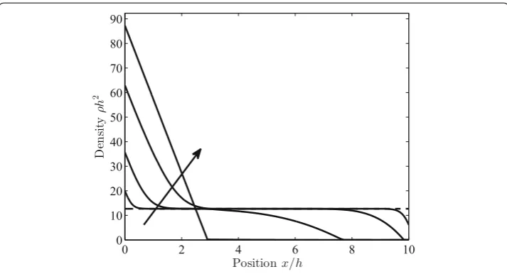
The length of the domain is L = 10h. First, a uniform distribution of positive walls is considered with an applied shear stress according toτ/G¯ = −1/20. This results in a pile-up of dislocation walls for which the evolution is shown in Fig.8. The applied stress pushes the dislocation walls towards the barrier, while at the same time the dislocation walls repel each other. This results in a pile-up against the barrier. The interaction stress emanates from the gradient of the density. In the final equilibrium state, this interaction stress must compensate the externally applied stress−τ which is constant. Therefore, a linear pile-up is predicted [21].
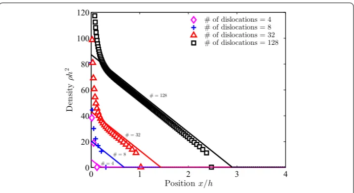
In Fig. 9, the equilibrium solution is shown for the present model and fully discrete simulations with different numbers of dislocations and thus initial densities. The results observed in Fig.9are consistent with the results found in [21]. The comparison between the continuum and discrete simulations is quite good for a large number of dislocations and at some distance from the barrier. However, if we decrease the number of walls below a certain limit, the continuum model no longer captures the discrete wall distribution, as the dislocations do not distribute linearly near the boundary. For all cases, the agreement in the region close to the boundary is poorer, because a boundary layer appears where the discrete nature of the dislocation walls is dominant. The assumptions made in deriving
Fig. 9 The pile-up of positive dislocation walls against an impenetrable barrier, predicted by the present continuum model and discrete dislocation simulations. The number of walls is varied
the continuum model do not hold in this region. In the expression for the velocity only the gradient of the density is related to the applied stress; therefore it is unable to capture the
1 √
x behaviour near the obstacle. However, the linear part of the pile-up, as explained in
[21], is captured accurately, i.e. the gradient of the density corresponds well between the discrete and continuum case. The absolute difference in density is a result of dislocation conservation in the domain. The area below the continuous and discrete data must be constant and equal. Because the continuum model is unable to capture the sharp peak near the boundary, the density in the region away from the boundary is higher.
Non-uniform distribution of positive and negative walls
To illustrate the effect of taking into account all short-range interaction stresses, and not only those between dislocations of the same sign, we consider equal numbers of positive and negative walls, corresponding in the continuum case with a distribution of SSDs, i.e.
ρ =ρSSD,κ = 0. Initially, these walls are not horizontally equispaced, but their mutual distances are such that they result in a non-uniform density distribution as illustrated by the dashed curve in Fig.10. In the center of our domain more walls are present, their number decreasing closer to the boundaries. The integral of the initial density profile corresponds with 89 dislocation walls. The boundaries are impenetrable barriers. No external stress is applied, such that the interactions between walls, due to the gradients in densities, constitute the only driving forces for dislocation motion. The length of the domain isL=60h.
In Fig.10, the evolution of the SSD density is shown. The driving force of the dislocation density, i.e. the gradient in the density profile, results in mutually repelling walls and the spreading of the density distribution. The density profile is evolving to its equilibrium configuration, i.e. a uniformly distributed dislocation density.
Fig. 10 The evolution of an initially non-uniformly distributed SSD density (dashed line). Due to the repulsive interaction stresses, the density profile evolves to a uniformly distributed density
Fig. 11 The steady state result of an initially non-uniformly distributed SSD density. The present model is here compared with discrete dislocation simulations and with a continuum model containing GND interactions only
density as a driving force for dislocation motion, which is obviously absent in the initial state. In the new, “all interactions” model the interactions between positive and negative walls is properly included via the gradient of the total dislocation density.
Outflow of dislocations
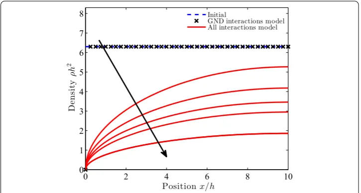
In the final example we replace the barrier atx=0 by a free outflow condition, regardless of the sign of the dislocations. A free boundary in the continuum framework is modelled by a Dirichlet condition on the densities, i.e.ρ(0)= κ(0)=0. Furthermore, no stress is applied and the length of the domain is set toL=10h. Our purpose is merely to illustrate the effect of accounting for all short-range dislocation interactions (as opposed to only GNDs) on the ability to model outflow. No comparison is therefore made with discrete simulations and only a qualitative analysis of the continuum models is performed.
Figure 12 shows a decrease in dislocation density near the boundary for the newly proposed model. The model with GND interactions only is unable to capture the outflow of dislocations, because there are no (gradients of) GNDs to generate the driving force in that formulation. In a qualitative sense the model presented here is thus capable of capturing dislocation outflow.
Conclusion and discussion
Starting from an idealised dislocation configuration, a continuum model for dislocation transport in single slip has been derived, including (short-range) dislocation-dislocation interactions. The driving force in the transport equations emanates from the behaviour of discrete dislocation walls. Whereas the long-range stresses in the driving force can be captured naturally in a continuum model, the short-range stresses are to be determined from the individual interactions between dislocations. These short-range stresses in the presented continuum model depend on the gradient of GND and total dislocation density, as opposed to other models found in literature in which they depend only on the gradient of GND density.
The resulting equations are non-linear transient PDEs. They are numerically solved by temporal and spatial discretisation and by adopting an incremental-iterative solution procedure. We develop a fully implicit scheme here, in contrast with the explicit time integration generally used in the literature. This framework was shown to convergence to a solution with a relatively low number of elements. In this study, no stabilisation is used for the transport equations, because this could interfere with the presence of the short-range dislocation interactions. When more realistic cases are considered, with larger problem length-scales, numerical stabilization may be necessary to avoid nonphysical solutions for tractable mesh sizes. Different approaches for stabilization of the dislocation transport equations as presented here (or similar) may be found in [22–24].
The behaviour of individual dislocation walls in a single slip system is captured ade-quately by our continuum model. However, a limitation of our model is its continuum nature, requiring a sufficient number of dislocation walls in the domain. A continuum description is unable to capture the distribution of dislocation walls when there is only a limited number of dislocations. The derivation of the interaction stress assumes that the walls are continuously distributed in the direction of the slip plane. In the case of a pile-up of walls against an impenetrable barrier, the linear part of the pile-up is captured accu-rately if the number of walls is sufficiently high. When the stress is removed in the case of a double pile-up, a continuum model cannot capture the discrete distribution when the number of dislocation walls is small.
It is shown that the short-range dislocation interactions can be easily implemented in an implicit finite element model for continuum dislocation transport. Although the current governing equations are formulated in terms of an idealised single-slip case, the ideas developed here may be extendable to more general cases with multiple active, and inter-acting, slip systems with mixed dislocations. As a first step, the extension to multiple slip systems with straight edge dislocations is considered in a forthcoming paper, assuming the Taylor-like organisation of the dislocations at the level of each individual slip system. This leads to balance laws for dislocation transport on each slip system which are equivalent with those for the single system considered here. The further extension to dislocations of mixed edge-screw type, cross-slip, etc. is a subject of further research.
Authors’ contributions
The theory regarding continuum dislocation transport was derived by MD, with input and suggestions from RP and MG to define the scope of the study. The implementation of dislocation transport in the continuum model and obtaining the simulation results were carried out by MD. The manuscript was drafted by MD. RP helped to draft the manuscript by providing input during the various stages of the drafting proces. Both RP and MG also contributed by critically revising the manuscript regarding both text and intellectual content. All authors read and approved the final manuscript.
Author details
1Materials innovation institute, P.O. Box 5008, 2600 GA Delft, The Netherlands,2Department of Mechanical Engineering, Eindhoven University of Technology, P.O. Box 513, 5600 MB Eindhoven, The Netherlands.
Acknowledgements
This research was carried out under the project number M22.2.09342 in the framework of the Research Program of the Materials innovation institute M2i (http://www.m2i.nl).
Competing interests
The authors declare that they have no competing interests.
References
1. Roters F, Eisenlohr P, Hantcherli L, Tjahjanto DD, Bieler TR, Raabe D. Overview of constitutive laws, kinematics, homog-enization and multiscale methods in crystal plasticity finite-element modeling: Theory, experiments, applications. Acta Mater. 2010;58(4):1152–211.
2. Lee EH. Elastic-plastic deformation at finite strains. J Appl Mech. 1969;36:1–6.
3. Rice JR. Inelastic constitutive relations for solids: an internal variable theory and its application to metal plasticity. J Mech Phys Solids. 1971;19:433–55.
4. Orowan E. Zur kristallplastizität. III: Über den mechanismus des gleitvorganges. Z Phys A-Hadron Nucl 1934; 89(9):634– 659.
5. Nye JF. Some geometrical relations in dislocated crystals. Acta Metall Mater. 1953;1(2):153–62. 6. Ashby MF. The deformation of plastically non-homogeneous materials. Philos Mag. 1970;21:399–424.
7. Shu JY, Fleck NA. Strain gradient crystal plasticity: size-dependent deformation of bicrystals. J Mech Phys Solids. 1999;47(2):297–374.
8. Gurtin ME. A gradient theory of single-crystal viscoplasticity that accounts for geometrically necessary dislocations. J Mech Phys Solids. 2002;50(1):5–32.
9. Menzel A, Steinmann P. On the continuum formulation of higher gradient plasticity for single and polycrystals. J Mech Phys Solids. 2000;48(8):1777–96.
10. Bargmann S, Ekh M, Runesson K, Svendsen B. Modeling of polycrystals with gradient crystal plasticity: a comparison of strategies. Philos Mag. 2010;90(10):1263–88.
11. Anand L, Gurtin ME, Lele SP, Gething C. A one-dimensional theory of strain-gradient plasticity: formulation, analysis, numerical results. J Mech Phys Solids. 2005;53(8):1789–826.
12. Ekh M, Grymer M, Runesson K, Svedberg T. Gradient crystal plasticity as part of the computational modelling of polycrystals. Int J Numer Meth Eng. 2007;72(2):197–220.
13. Evers LP, Brekelmans WAM, Geers MGD. Non-local crystal plasticity model with intrinsic SSD and GND Effects. J Mech Phys Solids. 2004;52(10):2379–401.
14. Roy A, Peerlings RHJ, Geers MGD, Kasyanyuk Y. Continuum modeling of dislocation interactions: why discreteness matters? Mater Sci Eng. A. 2008;486(1–2):653–61.
15. Groma I, Csikor FF, Zaiser M. Spatial correlations and higher-order gradient terms in a continuum description of dislocation dynamics. Acta Mater. 2003;51(5):1271–81.
16. Yefimov S, Groma I, van der Giessen E. A comparison of a statistical-mechanics based plasticity model with discrete dislocation plasticity calculations. J Mech Phys Solids. 2004;52(2):279–300.
17. Geers MGD, Peerlings RHJ, Hoefnagels JPM, Kasyanyuk Y. On a proper account of first- and second-order size effects in crystal plasticity. Adv Eng Mater. 2009;11(3):143–7.
18. Cleveringa HHM, van der Giessen E, Needleman A. Comparison of discrete dislocation and continuum plasticity predictions for a composite material. Acta Mater. 1997;45(8):3163–79.
19. Arsenlis A, Parks DM. Modeling the evolution of crystallographic dislocation density in crystal plasticity. J Mech Phys Solids. 2002;50(9):1979–2009.
20. Hirth JO, Lothe J. Theory of Dislocations. Florida: Krieger Publishing Company; 1992.
21. de Geus TWJ, Peerlings RHJ, Hirschberger CB. An analysis of the pile-up of infinite periodic walls of edge dislocations. Mech Res Commun. 2013;54:7–13.
22. Varadhan SJ, Beaudoin AJ, Acharya A, Fressengeas C. An analysis of the pile-up of infinite periodic walls of edge dislocations. Modelling Simul Mater Sci Eng. 2006;14:1245–70.
23. Kords C. On the role of dislocation transport in the constitutive description of crystal plasticity. PhD thesis, Rheinish-Westfälischen Technischen Hochshule Aachen, 2013.