Automatic tuning of the window size in the Box Car Back Slope
data compression algorithm
Jens Pettersson
a,1, Per-Olof Gutman
b,*aABB Corporate Research, 72178 V €
a
asteraas, Sweden
bDivision of Agricultural Engineering, Faculty of Civil and Environmental Engineering, Technion Israel Institute of Technology, Haifa 32000, Israel Received 3 February 2003; received in revised form 7 July 2003; accepted 31 July 2003
Abstract
In spite of the fact that there exist newer data compression algorithms with better compression ratios, the Box Car Back Slope (BCBS) algorithm is still offered by vendors of data acquisition systems and remains in use in many process industries. The as-sumption behind the BCBS algorithm is that the recorded process variable can be approximated by a piece-wise linear function, whereby variable values within a threshold window around the line segments are not stored. The window size is a critical parameter which should be selected such that a desired compromise between the data compression ratio and the approximation error is achieved. Based on a criterion function reflecting such a compromise, an automatic, recursive algorithm for tuning the BCBS threshold window size is presented in this paper. The algorithm has been used successfully to tune the window size for hundreds of process variables at the carton board manufacturing plant of Assi–Dom€aan Froovi, Sweden.€
Ó 2003 Elsevier Ltd. All rights reserved.
Keywords:Data compression; Box car back slope; Automatic tuning; On-line tuning; Process monitoring; Data processing; Threshold
1. Introduction
In process industries such as the pulp and paper in-dustry, thousands or ten of thousand variables are measured and stored. For most of these variables the sampling rate might be large, e.g. one reading/storage per minute. The data is used not only for immediate display on the operator monitors but is also saved for future reference and analysis. A typical storage period is one year. Even though computer storage media have become cheap and compact, the huge amount of data to be stored still necessitates the use of data compression algorithms whose purpose is to reduce the amount of stored data points while retaining the essential features of the measured signals.
This paper will concentrate on the Box Car Back Slope method (BCBS) [6], which is still widely used in
the process industry, despite of the fact that algorithms with better compression ratios have been developed during the last twenty years. In [17] a comparison is made between piece-wise linear compression methods, among them the swinging door algorithm, BCBS, the vector quantization method, the discrete cosine trans-form and a wavelet transtrans-form method, whereby the latter method is found to be superior. Also [1,10] found that wavelet transform methods are in general better than boxcar and other linear interpolation methods. Wavelet transforms are treated in many contributions, among them [1] where time varying wavelet packets are used, and [10] where a method is suggested to update the approximation coefficients each time a new data point arrives, and [15] where 2D wavelet analysis and com-pression is reviewed. Many other comcom-pression methods, and extensions of existing methods have been suggested over the last decade, e.g. Piece-wise Linear On-line Trending in [8], by clustering in [9], a spline-based method in [16], and based on neural networks in [14], to name just a few.
The BCBS is a real time algorithm, i.e. at sampling instantn, when the measured valueyðnÞis sampled, it is decided whether the pair ½ðn1Þ;yðn1Þ should be *
Corresponding author. Tel.: 829-2811; fax: +972-4-8295696.
E-mail addresses: [email protected] (J. Pettersson), [email protected] (P.-O. Gutman).
1
Fax: +46-21-323212.
0959-1524/$ - see front matter Ó 2003 Elsevier Ltd. All rights reserved. doi:10.1016/j.jprocont.2003.07.006
stored, or not. The BCBS contains no mechanism to post-process the data in order to change the stored data points. Hence the BCBS is a filter. It is obvious that better data reduction can be achieved with a computa-tionally more expensive smoothing or post-processing algorithm, which would require, however, that mea-sured data points be stored for some time. Wavelet methods belong to the latter category. Piece-wise linear compression methods, among them BCBS, require no data processing to display the approximant: the stored values are simply plotted against their time stamps. In contrast, transform based methods require the compu-tation of the inverse transform before display. The trade-off between inferior data compression but simple computations on one hand (e.g. BCBS), and superior
data compression but more complicated computations (e.g. wavelet methods) is something each user has to decide about.
The underlying assumption of the BCBS is that the signal itself (without measurement noise) can be well approximated by a piece-wise linear function and that the frequency of transitions from one line segment to another is considerably smaller than the measurement noise frequency. The crucial parameter of the BCBS is the threshold window size, h. If both yðnÞandyðn1Þ
fall within the current window(s),yðn1Þis not stored, otherwise yðn1Þ may be stored. An approximant of the original signal is then formed by linear interpolation of the stored values. The largerhis, the less data points will be stored and the less faithful the approximant will Nomenclature
a user set constant in the optimization algo-rithm, (16)
a user selected weight in optimization criterion b user set constant in the optimization
algo-rithm, (16)
c user set constant to randomize the update of dn, (22)
d factor multiplying the known or estimated measurement noise standard deviation, to calculate the window sizeh¼dr orh¼drr^ dn updated value ofdat the end ofTn, (16) and
(22)
eðtÞ approximation error¼yðtÞ ^yyðtÞ
^eeðtÞ estimate ofeðtÞ
Efg expected value
cn step size in the optimization algorithm, (16)
h BCBS window size ^
h
h optimal BCBS window size, (5)
Ln number of sub-intervals of un-stored
mea-surements inTn
k forgetting factor M lower limit forNn
Nn number of measurements duringTn
Nð0;r2Þ normal (Gaussian) distribution with mean¼0, and variance¼r2
mðtÞ measurement noise at sampling instantt p state variable of the BCBS algorithm PðÞ probability
q slope (in Back Slope mode) ^
q
qðtÞ estimate ofqat sampling instantt
r probability that a value is stored¼analytical data reduction ratio
rn data reduction ratio duringTn, (12)
rN data reduction ratio for a batch of N
mea-surements
RðeÞ analytical mean square of the approximation error
RnðeÞ mean square of the approximation error
duringTn
RNðeÞ sample mean square of the approximation
error forN measurements
Sn set of time-value pairs stored by the BCBS
algorithm duringTn
SN set of time-value pairs stored by the BCBS
algorithm, up to and including the sampling instantN, (1)
r standard deviation, or in particular, mea-surement noise standard deviation
^
r
r estimate of the standard deviation r r2ðyÞ analytical variance ofyðtÞ
r2
nðyÞ sample variance of yðtÞduringTn
r2
NðyÞ sample variance ofyðtÞoverN measurements
Rn sign of gradient ofVnwith respect tod, (15)
Tn nth time interval
VðhÞ analytical window size optimization criterion Vn window size optimization criterion value
ac-cumulated duringTn, (11)
VNðhÞ window size optimization criterion for a
batch ofN measurements, (4) wn random Gaussian number, (22)
wðtÞ dummy variable at sampling instant t in the definitions of BCwindow and BSwindow in Eqs. (2) and (3), respectively
xðtiÞ ¼yðtiÞ yðti1Þ ¼the difference between two subsequent measurements
yðtÞ measured process value at sampling instant t ^
be. The window size plays the same r^oole in other piece-wise linear compression methods, see e.g. [8], while for transform methods a threshold has to be decided upon to determine which coefficients to include in the ap-proximant.
Our experience with the application of BCBS on the carton board machine at Assi–Dom€aan Fr€oovi, Sweden, shows that for many measured signals, BCBS with a threshold window size approximately equal to four noise standard deviations achieves satisfactory signal ap-proximation with only about 10% of the original data. It is however easy to synthesize noisy signals for which this rule of thumb gives too modest a data reduction.
It is impossible to tune the window size manually for thousands of signal channels. In most of themhremains at its default start up setting, e.g. 1% of the allowed signal span which may be much larger than the actual measured signal variation. The experience at Assi– Dom€aan Fr€oovi shows that the result may be that almost no data points are stored.
Several attempts have been made to automatically tune the crucial tuning parameter(s) of various com-pression algorithms. In [8] the variance of the measured process variable, including the measurement noise, is estimated on-line and used to adjust the threshold win-dow size. Automatic tuning of the winwin-dow size of the BCBS algorithm is proposed in chapter 8 in [12] and in [13], on which this paper is based. A criterion based on the deviation of the approximant from the measured signal is proposed for on-line wavelet data compression to adaptively calculate the thresholds in [11].
In this paper we propose an algorithm to automati-cally tune the BCBS threshold window size. This is a non-trivial problem even if the measurement noise standard deviation were known, as indicated above. The algorithm is based on the minimization of a criterion that weighs the data reduction and the deviation of the approximant from the measured signal. The criterion is estimated during each piece of the piece-wise linear ap-proximant, and a modified descent search is performed to find the optimal threshold window size.
The paper is organized as follows. As a service to the reader, the BCBS algorithm is defined in Section 2. A full description can be found in e.g. [6] or [17]. An detailed example of the functioning of the algorithm is also found in [13]. In Section 3, a preliminary off-line tuning algorithm is suggested, and analyzed for the simple case of a constant process signal with identically independent Gaussian measurement noise, leading up to the proposed on-line tuning algorithm in Section 4. In Section 5, the algorithm is demonstrated on a syn-thetic signal, as well as on a measured process variable from Assi–Dom€aan Fr€oovi. Some conclusions are drawn in Section 5. Appendix A contains pseudo-code for the full algorithm. A list of symbols is found in nomen-clature.
2. The Box Car Back Slope algorithm
Assume without loss of generality that the sampling period equals one and that the sampling instants are t¼1;2;3;. . .. Let the current sampling instant bet¼n, with nP3. The measured scalar data up to and in-cluding the current sampling instant are denoted yð1Þ; yð2Þ;. . .;yðN1Þ;yðNÞ. The set of stored data, in the form of time-value pairs, up to and including the current sampling instant, is
SN ¼ ½ft1;yðt1Þ;½t2;yðt2Þ;. . .;½tm1;yðtm1Þ;½tm;yðtmÞg;
ð1Þ
where ft1;t2;. . .;tmg f1;2;3;. . .;N1g, m is a
in-creasing function ofN, and in particularm6N1. The
BCBS algorithm is initialized witht1¼1 andt2¼2. There are two time dependent threshold windows in the BCBS algorithm: the Box Car window (BCwindow), and the Back Slope window (BSwindow). The windows are defined as the following sets:
BCwindow¼fwðtÞ 2RjyðtmÞh6wðtÞ6yðtmÞ
þh;tPtmg ð2Þ
BSwindow¼ wðtÞ 2RjyðtmÞ
h
þyðtmÞ yðtm1Þ
tmtm1
ðttmÞ
6wðtÞ6yðtmÞ þh
þyðtmÞ yðtm1Þ
tmtm1
ðttmÞ;tPtm
ð3Þ
wherehis the threshold window size. The windows will form strips when displayed in the ½t;yðtÞ-plane. The height of the window intersected along the y-axis is 2h for eachtPtm.
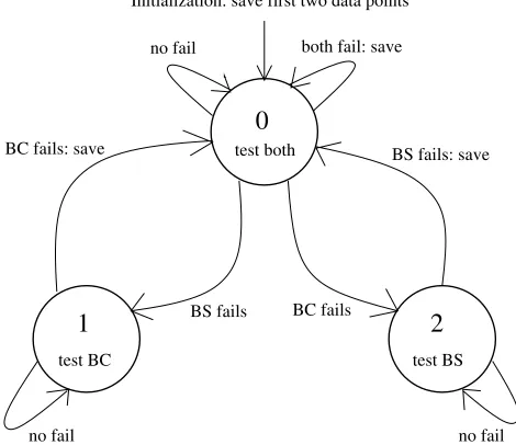
A threshold window is said to be active if the in-coming measurement, yðnþ1Þand its predecessor yðnÞ
are tested against it: theBox Car testfails if at least one of two measurements does not belong to BCwindow, and, the Back Slope test fails if at least one of the two measurements does not belong to BSwindow. Which windows are active depends on the state p that may assume the values 0 (both windows are active), 1 (BCwindow active), and 2 (BSwindow active). The state transition diagram is found in Fig. 1.
The algorithm is initialized withp¼0. When p¼0 the state remains unchanged as long as the incoming measurement yðnþ1Þ and its predecessor yðnÞ both belong to BCwindow and to BSwindow, or both of the windows fail the two tests. In the latter case, denoted as ‘‘both fail’’ in Fig. 1,½n;yðnÞis appended toSnþ1, unless
fails, p returns to 0 and ½n;yðnÞ is appended to Snþ1.
When p¼0, and the Box Car test fails, p becomes 2, and BCwindow ceases to be active. As long as the Back Slope test does not fail the state remains p¼2. When the Back Slope test fails, p returns to 0 and ½n;yðnÞ is appended to Snþ1. Clearly, when data is appended to
Snþ1,mis increased by one, and the windows change. A
numerical example of the BCBS algorithm is found in e.g. [13].
3. An off-line algorithm for determining the threshold window size
It was stated above that the Box Car Back Slope al-gorithm is a filter, implying that measured consecutive data are not saved temporally for post-processing. It is however instructive to investigate, a posteriori, how the threshold window size should have been chosen if a batch of measured data were at hand, in order to de-velop an efficient window sizing algorithm.
Assume therefore that a batch of N measurements have been recorded, and that it is desired to select the stored data set, SN (1) with the Box Car Back Slope
algorithm. Since the window size h reflects a trade-off between the data reduction ratio and the goodness of the approximant, it is natural to choose hsuch that an ap-propriate criterion is minimized, see the discussion in [1]. In this section, a criterion will be proposed and analysed in a simple case, for which also a numerical example is given.
Define eðtÞ ¼yðtÞ ^yyðtÞ as the approximation error at timet, whereyðtÞis the measured value, and^yyðtÞthe BCBS generated approximant. Let RN ¼P
N t¼1e
2ðtÞ=N be the sample mean square of the approximation error.
Let rN ¼cardSN=N define the data reduction ratio,
where card SN denotes the number of stored pairs inSN,
i.e. half the amount of numbers actually stored. An appropriate criterion is then
VNðhÞ ¼ ð1aÞrNþa
RNðeÞ
r2
NðyÞ
ð4Þ
where a2 ð0;1Þ and r2
NðyÞ ¼
PN t¼1½y
2ðtÞ ðPN t¼1yðtÞÞ
2 = N=ðN1Þis the sample variance of yðtÞ. The value of the constantais chosen by the user to reflect the trade-off between data reduction and the reproduction of the original signal. For example,aclose to 0 will emphasize data reduction. The window size is then found from
^ h
h¼arg min
h VNðhÞ ð5Þ
3.1. Analysis of VN in a simple case
We will now analyze the exact expression of VNðhÞ,
given a set of data in a simple case. In order to simplify the calculations we consider here only the Box Car al-gorithm, and in particular the trueBox Car algorithm, i.e. when only the value that fails the boxcar test is stored and the data reproduction is done by zero-order holding of each stored value. A similar analysis may be undertaken for the BS and BCBS algorithms.
Consider the case when yðtÞ 2Nð0;r2Þ, t¼1; 2;. . .;N, meaning that for eacht,yðtÞis an independent Gaussian random variable with zero mean, and vari-ance¼r2. The interpretation is that the true process value is zero, with added Gaussian measurement noise. Assume that some value, yðt0Þ, at time t0 was stored. Then we are interested in the probability that yðtkÞ,
wherekP1 will be stored. We are also interested in the variance of the error eðtkÞ if yðtkÞ is not stored. Since
yðt0Þ and yðtkÞ are independent, the random variable
zðtkÞ ¼yðtkÞ yðt0Þ 2Nð0;2r2Þ. Now, let r¼PðstoreÞ, i.e. the probability that a value is stored which equals the analytical data reduction ratio in this case. Thus,
PðstoreÞ ¼PðjzðtkÞj>hÞ
¼1 1
2rpffiffiffip Z h
h
ex2=ð4r2Þdx
¼1erfðh=2rÞ ð6Þ
For the error,eðtkÞ, we have
eðtkÞ ¼
zðtkÞ if jzðtkÞj<h
0 otherwise
The statistical properties of the error are then
EfeðtkÞg ¼
1 2rpffiffiffip
Z h
h
xex2=ð4r2Þ
dx¼0 ð7Þ
and test both
0
2
1
test BC test BS
no fail no fail
both fail: save no fail
BC fails
BS fails: save Initialization: save first two data points
[image:4.595.51.286.76.279.2]BS fails BC fails: save
Efe2ðtkÞg ¼
1 2rpffiffiffip
Z h
h
x2ex2=ð4r2Þ dx
¼ 2rffiffiffi p
p rpffiffiffiperfðh=2rÞheh2=4r2 ð8Þ
where erfðxÞ ¼ ð2=pffiffiffipÞR0xex2dx. Hence, the analyti-cal mean square of the approximation error is RðeÞ ¼
Efe2ðt
kÞg.
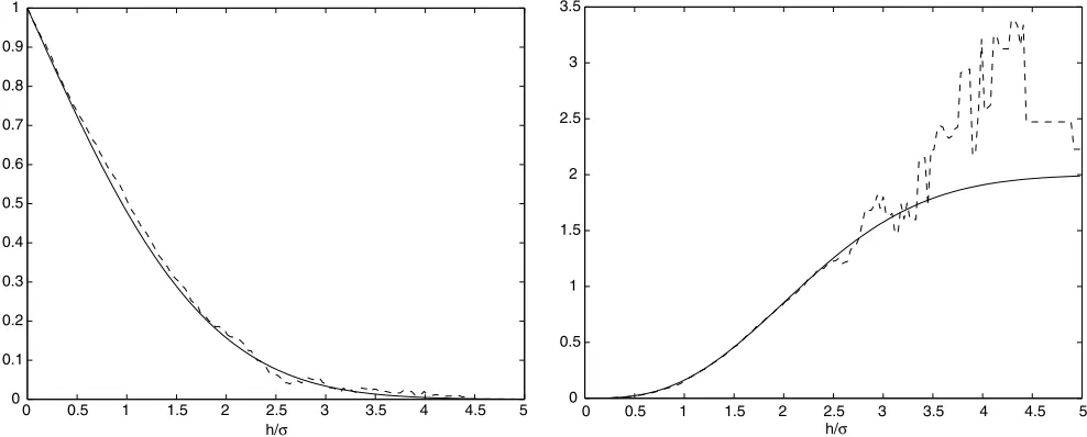
In Fig. 2 the analytical functions for r and R2ðeÞ=
r2ðyÞare plotted versush=r, together with the calculated values ofrN and R2NðeÞ=r
2
NðyÞ, respectively, from a
nu-merical simulation ofyðtÞwithN ¼1000. We notice that the analytical functions are smooth and hence the ana-lytical criterion corresponding to (4),VðhÞ ¼ ð1aÞrþ
aRðeÞ=r2ðyÞ will have one global minimum for every choice ofa2 ð0;1Þ. The curves from the simulation are almost equal to the analytical curves for smallh, while they exhibit large peaks for higher values of h, where few values are stored. Larger N will give smoother curves. Hence, VN may have many local minima for
finite N which will complicate the search for its global minimum.
4. An on-line algorithm for determining the threshold window size
In this section, we present an on-line algorithm that adaptively tunes the threshold window sizeh. In agree-ment with the basic assumption behind the use of BCBS, as mentioned in the Introduction, we assume that the signal yðtÞ can be described by a low frequency signal with an additive independent Gaussian measurement
noise, i.e. yðtÞ ¼y0ðtÞ þmðtÞ, where y0ðtÞ is the ‘‘true’’ signal andmðtÞ 2Nð0;r2Þ. Ifrwere known, an intuitive choicehwould beh¼drwhere the constantd would be equal to, say 4, since otherwise a too low data re-duction will be achieved, see Fig. 2. Compare the anal-ysis in [8]. On the other hand, a higher value ofd might be bad, since it could give poor reproduction of the original signal.
A first step in the on-line algorithm is thus to estimate the unknown measurement noise standard deviation r. This is done by introducing the random processxðtiÞ ¼
yðtiÞ yðti1Þ. Since we have assumed thaty0ðtÞis a low-frequency signal, y0ðtiÞ y0ðti1Þ andxðtiÞ 2 Nð0;2r2Þ.
The estimaterr^can be calculated in a recursive manner by
^
r
r2ðtiÞ ¼krr^2ðti1Þ þ ð1kÞx2ðtiÞ=2 ð9Þ
where the forgetting factor k typically is 0.95–0.99 [7]. The use of a forgetting factor makes it possible to handle also time varying noise.
Estimation according to (9) may give a large bias in the case of a signal with a slope. However, the slope is detected by the BCBS-algorithm. Therefore, in Back Slope mode, the estimaterr^can be modified by assuming yðtÞ ¼q ðtt0Þ þy0þmðtÞ. Here the timet0is when the BCBS algorithm enters the Back Slope mode, q is the slope and y0 is a constant. NowxðtiÞ ¼yðtiÞ yðti1Þ ¼ q ðtiti1Þ þmðtiÞ mðti1Þ. Assume as above that the time is normalized so that titi1¼1, then xðtÞ 2
Nðq;2r2Þ. The recursive estimate of ris now
^ q
qðtiÞ ¼^qqðti1Þ þ1=ðtit0Þ xðtiÞ
h
^qqðti1Þ
i
^
r r2ðt
iÞ ¼krr^2ðti1Þ þ ð1kÞ xðtiÞ
h
^qqðtiÞ
i2. 2
ð10Þ
0 0.5 1 1.5 2 2.5 3 3.5 4 4.5 5 0
0.1 0.2 0.3 0.4 0.5 0.6 0.7 0.8 0.9 1
h/σ
0 0.5 1 1.5 2 2.5 3 3.5 4 4.5 5 0
0.5 1 1.5 2 2.5 3 3.5
[image:5.595.45.539.73.272.2]h/σ
Fig. 2. Analytical values (solid lines) ofr(left) andR2ðeÞ=r2ðyÞ(right) together with simulated values (dashed lines) ofr
N (left) andR2NðeÞ=r2NðyÞ
Eq. (10) is initialized with ^qqðt0Þ ¼xðt0Þ, and ^qqðtiÞ and
^
r r2ðt
iÞ are updated until a recording is made and the
BCBS algorithm leaves the Back Slope mode.
We now have the estimate rr^ of the measurement noise standard deviation. The question then is how to choose the factord. As mentioned in Section 1 using the ad hocd¼4 may give either poor data reproduction or poor data reduction. Instead,dmay be chosen such that the criterion in Eq. (4) is minimized. The minimization can be done on-line by any recursive minimization al-gorithm [4]. We choose the one presented in [2] which is now described as applied for our problem.
Let us divide the time line into intervals, such that the nth time interval is Tn¼ ½Tnþ1;Tnþ1 with Tnþ1Tn¼
Nn, and with the provision thatyðTnþ1Þis stored by the BCBS algorithm, and that Tn contains LnP1
sub-intervals of un-stored measurements.
By similarity with the criterion (4) in the off-line case, we define Vn to be the value of the criterion computed
duringTn:
Vn¼ ð1aÞrnþa
RnðeÞ
r2
nðyÞ
ð11Þ
wherea2 ð0;1Þis the user chosen tuning constant,
rn¼Sn=Nn ð12Þ
is the data reduction ratio overTn, with Sn¼cardSNn,
see (1),
RnðeÞ ¼
XTnþ1
t¼Tnþ1
e2ðtÞ=N
n ð13Þ
is the mean square of the approximation error overTn,
and
r2
nðyÞ ¼
1 Nn1
XTnþ1
t¼Tnþ1
y2ðtÞ
2
4 1
Nn
XTnþ1
t¼Tnþ1
yðtÞ
!23
5 ð14Þ
is the sample variance ofyðtÞoverTn.
Note that Vn is a function of the window size h, and
since we leth¼drr^,Vnis a function ofd. Hence we aim
to minimizeVn with respect tod.
Assume thatd ¼dnduringTn, and thatd is updated
after each time intervalTn. Let
Rn¼sign
VnVn1 dndn1
: ð15Þ
The recursive algorithm for updatingd is then
dnþ1¼dncnRn ð16Þ
with
cn¼ bcn1 if RnRn1¼ 1 acn1 otherwise
andc0>0. In [2] a value set forfa;bgis given for which the algorithm converges to the minimum of the crite-rion.
To use this recursive minimization algorithm, we must calculateVnfor the time intervalTnwithout storing
any more values then stored by the BCBS algorithm. First we will consider the mean square of the ap-proximation error,RnðeÞ, (13) for which it is essential to
calculate PTnþ1
t¼Tnþ1e
2ðtÞ. Consider the jth out ofL
n
sub-intervals of un-stored measurements inTn. Let the
sub-interval be such that measurements are stored at timet0 andtkand that no values are stored in betweent0andtk.
At time ti, wheret0<ti<tk, we naturally do not know
neither the timetk, nor the value ofyðtkÞ. We therefore
introduce the estimated error at time ti,
^
eeðtiÞ ¼yðtiÞ yðt0Þ ð17Þ
The real error,eðtiÞ, after the BCBS algorithm has stored
the value at time tk and interpolated between yðt0Þand yðtkÞ, is given by
eðtiÞ ¼yðtiÞ ðtit0Þ
yðtkÞ yðt0Þ tkt0
yðt0Þ ð18Þ
Now, lets¼ ðyðtkÞ yðt0ÞÞ=ðtkt0Þandi¼tit0, then
eðtiÞ ¼^eeðtiÞ is ð19Þ
Then
Xk1
i¼0
e2ðtiÞ ¼
Xk1
i¼0
^ee2ðtiÞ þ2s
Xk1
i¼0
i^ee2ðtiÞ þ
k3 3 k 2 2 þ k 6 s
2
ð20Þ
The sums Pki¼01^ee2ðt
iÞ and P k1
i¼0i^eeðtiÞ can be computed
recursively, for example, Pki¼01i^eeðtiÞ ¼ ðk1Þ^eeðtk1Þ þ
Pk2
i¼0 i^eeðtiÞ. At timetk, when the recording is made,sand
kbecome known, andRj¼P k1
i¼0e 2ðt
iÞcan be calculated.
Thus, the total mean square error duringTn is
RnðeÞ ¼
1 Nn
XLn
j¼1
Rj: ð21Þ
We also need to calculate the sample variance r2
nðyÞ
duringTn, see (14). Here,P Tnþ1
Tnþ1y
2ðtÞandPTnþ1
Tnþ1yðtÞcan
be computed recursively.
The number of stored values duringTn,Sn, is simply
calculated by lettingSn¼Snþ1 if a value is stored. The
data reduction ratio is then given by (12). Finally, at timeTnþ1, i.e. at the end ofTn,Vnis calculated according
to (11).
During simulations of the on-line tuning algorithm, it became evident that the search algorithm may find a local minimum. The reason for this is that Vn is
reali-zation dependent. This was solved by (a) choosing Nn>MwhereMis large enough to makeVnsmooth and
(b) by modifying Eq. (16) in a way similar to the func-tioning of simulated annealing, or genetic algorithms [3], or other random search algorithms [5] that ensure con-vergence to the global minimum,
wherecis a user selected constant andwn2Nð0;1Þis a
random Gaussian number. The search algorithm will thus always take a step in some direction and eventually find a global minimum.
In Appendix A the full on-line tuning algorithm is shown in pseudo-code.
4.1. Numerical evaluation
In order to verify that the proposed algorithm func-tions as expected, it was applied to measured process data and to artificial data. The following numerical parameter values were used in the algorithm: k¼0:95, M ¼600, a¼1:2,b¼0:5,c¼0:2, anda¼0:01.
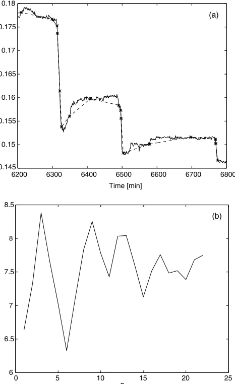
In Fig. 3a, a sequence from one of the Assi–Dom€aan Fr€oovi process signals is shown, together with the stored values, and the reproduced signal interpolated from the
stored values. Clearly the tuning algorithm finds a threshold window size h which captures most of the variation in the original signal without storing too many values. For this particular signal a compression ratio of 99% was achieved. Values ofdare presented in Fig. 3b. The algorithm converges to d7:5.
Although oscillating signals are hopefully not rep-resentative for the process industry, we chose as the second test signal a pure sinus signal without noise. Such a signal would be suitable for a transform based compression method; ideally only 4 numbers need to be stored, namely the start time (or, alternatively, the stop time) of the sinusoidal interval, the frequency, the amplitude and the phase. It is interesting to see how BCBS together with the tuning algorithm handles this case. The result of the simulation is shown in Fig. 4a
6200 6300 6400 6500 6600 6700 6800 0.145
0.15 0.155 0.16 0.165 0.17 0.175 0.18
Time [min]
0 5 10 15 20 25
6 6.5
7
7.5
8
8.5
n
(a)
[image:7.595.307.541.285.677.2](b)
Fig. 3. Application of the BCBS tuning algorithm on a process signal from Assi–Dom€aan Fr€oovi. In (a) the original signal (solid line), stored values (‘‘*’’) and reproduced signal (dashed line) are shown. The re-produced signal is close to the original signal. In (b) the values ofdare displayed.
2.8 2.805 2.81 2.815 2.82 2.825 x 10⁴ –1
–0.8 –0.6 –0.4 –0.2 0 0.2 0.4 0.6 0.8 1
Time [min]
(a)
(b)
0 5 10 15 20 25 30 35 40 45 50 6
7 8 9 10 11 12 13
[image:7.595.46.279.294.675.2]n
and one sees that the interpolated signal would capture most of the variations in this signal, too, by storing 12 points per period, in steady state. Also,d converges to a higher value in this case, see Fig. 4b. It is easy to show that BCBS without tuning of the window size would in general be less efficient: either by storing more points, or by representing the sinusoid poorly. A more complete picture of the frequency domain properties of the boxcar and backslope algorithms is given in [10], where the frequency functions from two sets of process data to their respective compressed data sets are computed using the describing function method.
5. Conclusions and discussion
The performance of the BCBS algorithm depends strongly on the chosen threshold window size h. Too small a window will result in a low data reduction ratio, while a too large window will result in loss of informa-tion.
An on-line tuning algorithm for the window size was proposed. The tuning algorithm first estimates the measurement noise, then chooses the window size as a factor times the estimated measurement noise. The fac-tor is chosen by recursively minimizing a loss function that reflects the desired compromise between data compression ratio and approximation error.
The parameters of the tuning algorithms have differ-ent influence and may partly be chosen independdiffer-ently of each other. a characterizes the loss function. a and b determines the bandwidth and transient properties of the optimization routine itself.k,M, andcinfluence the convergence rate and the sensitivity to changing signal characteristics.
Hence, to use the automatic tuning algorithm re-quires the user to choose values for the six parameters,
k,M,a,b,c, anda. In contrast, manual tuning demands the tuning of the threshold window size itself,h, for each and every process variable. Clearly, if six parameters would have had to be set for each process variable, the tuning algorithm proposed here would have been ex-tremely disadvantageous. However, our experience from Assi–Dom€aan Fr€oovi shows that after some initial exper-imentation, the same six parameter values can be used for all process variables. Therefore, great savings are achieved by automatic on-line tuning.
At Assi–Dom€aan Fr€oovi the window sizes for the BCBS recording of hundreds of process variables have been tuned automatically. It was found that the tuning could be performed sequentially on one process variable at a time, i.e. after the convergence of the window size of one variable, the automatic tuner was directed (automati-cally) to the next. In this way, the computational over-head was kept very low.
In addition to on-line tuning algorithms, we believe that process information systems using the BCBS algo-rithm must utilize some kind of fault diagnosis function. For example, we showed in this paper that it is possible to calculate recursively the statistics of the error for the reproduced signal. These statistics could then be pre-sented to the user of the reproduced signal, such that she/he gets an estimate of the accuracy of the signal. It would also be possible to include alarm functions, which warn when the error becomes too large or the reduction ratio becomes too small, indicating that the threshold window size must be re-tuned. Outlier handling could be included in a similar way. The latter idea is pursued in e.g. [8] for another piece-wise linear compression algo-rithm.
Appendix A. Algorithm for on-line tuning of the Box Car Back Slope algorithm
We will now show the full algorithm for the on-line tuning of the threshold windowh.
Initialize all variables
repeat until
[store,p]¼BCBStestðyðtÞ;t;. . .;pÞ
ifstore rn:¼rnþ1
ifi>1
s:¼ ðyðt1Þ yðtrÞÞ=i
Rj¼RjþR^ee2þ2sRi^eeþ k 3 3
k2 2 þ
k
6
s2 i:¼0
R^ee2 :¼0
Ri^ee:¼0
end
^ m
m:¼0;tm:¼0
ifMn>M
Re :¼Rj=Mn
rn:¼rn=Mn
r2
y :¼
Ry2 ðRyÞ
2 =Mn
=ðMn1Þ
Vn:¼ ð1aÞrnþaRe=r2y
Sn:¼signððVnVn1Þ=ðdndn1ÞÞ
ifSnSn1¼1
cn:¼acn1
else cn:¼bcn1
end
dnþ1:¼dncnSnþcwn
dn1:¼dn;dn:¼dnþ1 Sn1:¼Sn;Sn:¼Snþ1 Vn1:¼Vn
rn:¼0;En:¼0
Ry2:¼0;Ry :¼0
end end else
ifp¼1 ^
r
r2:¼krr^2þ ð1kÞz2=2 h:¼dpffiffiffiffiffirr^2
end ifp¼2
tm:¼tmþ1
^ m
m:¼mm^þ1=tmðzmm^Þ
^
r
r2:¼krr^2þ ð1kÞðzmm^Þ2 =2 h:¼dpffiffiffiffiffirr^2
end
Mn:¼Mnþ1;i:¼iþ1
^ee:¼yðtÞ yðtrÞ
R^ee2:¼R^ee2þ^ee2
Ri^ee :¼Ri^eeþi^ee
end
Ry:¼RyþyðtÞ
Ry2 :¼Ry2þyðtÞ2
end
References
[1] B.R. Bakshi, G. Stephanopoulos, Compression of chemical process data by functional approximation and feature extraction, AIChE J. 42 (2) (1996) 477–492.
[2] C.G. Baril, P.-O. Gutman, Performance enhancing adaptive friction compensation for uncertain systems, Trans. Control Syst. Technol. 5 (5) (1997) 465–479.
[3] L.J. Fogel, A.J. Owens, M.J. Walsh, Artificial Intelligence through Simulated Evolution, Wiley, New York, 1966.
[4] G.E. Forsythe, M.A. Malcolm, C.B. Moler, Computer methods for mathematical computations, Prentice-Hall Series in Automatic Computation, Englewood Cliffs, NJ, 1977.
[5] P.-O. Gutman, J.J. DiStefano, Parameters of thyronine metabo-lism (T3, T4, RT3) from normal and pathological human data:
Some numerical results concerning parameter estimates their variability and their possible utility in diagnostic classification, UCLA Biocybernetics Lab. Report 77-1, UCLA-ENG-7730, University of California, Los Angeles, 1977.
[6] J.C. Hale, H.L. Sellars, Historical data recording for process computers, Chem. Eng. Prog. 37 (11) (1981).
[7] L. Ljung, System Identification, Theory for the user, Prentice Hall, 1987.
[8] R.S.H. Mah, A.C. Tamhane, S.H. Tung, A.N. Patel, Process trending with piece-wise linear smoothing, Comput. Chem. Eng. 19 (2) (1995) 129–137.
[9] K.J. Mo, S. Eo, D. Shin, E.S. Yoon, Qualitative interpretation and compression of process data using clustering method, Comput. Chem. Eng. 22 (Suppl. S) (1998) 555–562.
[10] M. Misra, S.J. Qin, S. Kumar, D. Seemann, On-line data compression and error analysis using wavelet technology, AIChE J. 46 (1) (2000) 119–132.
[11] M. Misra, S. Kumar, S.J. Qin, D. Seemann, Error based criterion for on-line wavelet data compression, J. Process Control 11 (6) (2001) 717–731.
[12] J. Pettersson, On Model Based Estimation of Quality Variables for Paper Manufacturing. Licentiate Thesis, ISSN 0347-1071. Department of Signals, Sensors and Systems, Royal Institute of Technology, Stockholm, Sweden, 1998.
[13] J. Pettersson, P.-O. Gutman, Automatic tuning of the window size in the Box Car Back Slope data compression algorithm, in: Proceedings of the 7th IEEE Mediterranean Conference on Control and Automation, Haifa, Israel, 1999.
[14] H. Teng, H.B. Du, P.J. Yao, Prediction of process trends based on neural networks, Chin. J. Chem. Eng. 10 (3) (2002) 286–289. [15] J. Trygg, N. Kettaneh-Wold, S. Wallbacks, 2D wavelet analysis
and compression of on-line industrial process data, J. Chemom. 15 (4) (2001) 299–319.
[16] H. Vedam, V. Venkatasubramanian, M. Bhalodia, A B-spline based method for data compression, process monitoring and diagnosis, Comput. Chem. Eng. 22 (Suppl. S) (1998) 827–830. [17] M.J. Watson, A. Liakopoulos, D. Brzakovic, C. Georgakis, A