WORKING PAPER NO. 150
EQUITY AND BOND
MARKET SIGNALS AS
LEADING INDICATORS OF
BANK FRAGILITY
BY REINT GROPP,
JUKKA VESALA AND
GIUSEPPE VULPES
June 2002
E U R O P E A N C E N T R A L B A N K
WORKING PAPER NO. 150
EQUITY AND BOND
MARKET SIGNALS AS
LEADING INDICATORS OF
BANK FRAGILITY
BY REINT GROPP,
JUKKA VESALA AND
GIUSEPPE VULPES
*June 2002
* Research assistance by Sandrine Corvoisier and Roberto Rossetti is gratefully acknowledged. The views expressed in this paper are solely those of the authors and not those of the ECB. We thank Allen Berger, Jürg Blum, Max Bruche, Vitor Gaspar, Christopher James,
E U R O P E A N C E N T R A L B A N K
© European Central Bank, 2002
Address Kaiserstrasse 29
D-60311 Frankfurt am Main Germany
Postal address Postfach 16 03 19
D-60066 Frankfurt am Main Germany
Telephone +49 69 1344 0
Internet http://www.ecb.int
Fax +49 69 1344 6000
Telex 411 144 ecb d
All rights reserved.
Reproduction for educational and non-commercial purposes is permitted provided that the source is acknowledged. The views expressed in this paper are those of the authors and do not necessarily reflect those of the European Central Bank.
Contents
Abstract
4
Non-technical summary
5
1.
Introduction
6
II.
Properties of market indicators
8
II.A Equity-based indicators
9
II.B Subordinated debt-based indicators
11
II.C Impact of the safety net
14
III.
Empirical implementation
16
III.A Measurement of bank failures
16
III.B Market indicators
17
III.C Expectation of public transport
19
III.D Sample selection
19
IV
Descriptive statistics
20
V
Empirical estimation
21
V.A Estimation methods
21
V.B Logit-estimation results
22
V.C Hazard-estimation results
23
VI. Robustness and extensions
26
VII. Conclusion
29
Literature
31
Tables & charts
34
Appendices
52
Abstract
We analyse the ability of the distance-to-default and bond spreads to signal bank fragility. We show that both indicators are complete and unbiased and that spreads are non-linear in the probability of bank default. We empirically test these properties in a sample of EU banks. We find leading properties for both indicators. The distance-to-default exhibits lead times of 6 to 18 months. Spreads have signal value close to default only, in line with the theory. We also find that implicit safety nets weaken the predictive power of spreads. Further, the results suggest complementarity between both indicators, reducing type I errors. We also examine the interaction of the indicators with other bank information.
JEL codes: G21, G12
Non-technical summary
This paper examines whether forward-looking indicators of bank soundness could be constructed using financial market data on the securities issued by banks. There is
considerable interest on the issue, since market data are available on a high frequency, compared with profit and loss accounts and balance sheets. So far, all empirical evidence has focused on banks’ subordinated bond spreads. In this paper, we also examine the properties of an equity market-based indicator, the distance-to-default, and compare its properties to those of the spread. The main contributions of the paper are (i) a theoretical examination of the predictive properties of the two indicators, (ii) the estimation of a proportional hazard model to test these properties, making efficient use of the information contained in the prevalence of an indicator over time, and (iii) an explicit test for the role of the public safety net in the information content of market indicators.
Using a standard option pricing framework, we show that the equity-based distance-to-default and the subordinated bond spread have two highly desirable properties to be leading indicators of bank fragility. They are complete in the sense that they reflect the three major determinants of default risk (earnings expectations, leverage and asset risk) and unbiased in the sense that they reflect these risks correctly. However, the theory also suggests that the two indictors exhibit important differences in their predictive ability. In particular, we show that the response of the spreads to an increase in default probability is non-linear, with little response relatively far away from default and a strong reaction close to default. This also implies that the distance-to-default should deliver an earlier signal of fragility than the spread.
In our empirical implementation, we calculate distances-to-default and subordinate debt spreads for European banks for which suitable data is available for the period 1991-2001. For spreads, we focus on secondary market spreads on adequately large bond issues in order to abstract from noise due to limited liquidity. We use two different econometric models: a logit model, which we estimate for different time horizons (3-24 months ahead of default) and a proportional hazard model. The proportional hazard model permits conditional predictions of failure. The conditional predictions are based on having “survived” to a certain point in time, with a certain value of the market indicators in the previous period. Hence, the hazard model allows analysing the importance of the persistence of the market signals. We also test the additional information contained in market indicators compared with bank accounting information and ratings, as well as the impact of the expectation of public support on the signal value obtainable from the market data. In the empirical implementation we were faced with the problem that in Europe, very few banks – formally – declare bankruptcy. However, we circumvented this problem by using the downgrading of a bank to below C in the Fitch/IBCA individual rating (a rating that excludes the safety net) and which is intended to signal a material weakening in the stability of the bank. When examining the subsequent performance of the bank, we found that in virtually all cases, either public intervention or major restructuring took place six to twelve months after the downgrade.
Our empirical results support the theory. Both indicators are found to have predictive power for bank fragility. Further, the spread typically only reacts quite close (3 to 6 months) to default, whereas for the distance to default, we find predictive power as far from default as 24 months. We also find strong support for the notion that the information content of spreads is significantly diminished in the case of banks, which markets expect to be bailed out in case of difficulties. The equity-based distance-to-default does not appear to suffer from this shortcoming.
As regards the relationship of the two market indicators with several other sources of bank specific information, we find, one, that the market indicators contain additional
I.
Introduction
From a supervisory perspective the securities issued by banks are interesting for two reasons: First, market prices of debt and equity may increase banks’ funding cost and, therefore, induce market discipline, which may complement traditional supervisory practices (such as capital requirements and on-site inspections) in ensuring the safety and soundness of banks. The market may play a particularly useful role in disciplining the risks of large, complex and internationalised banking organisations. Second, supervisors are considering the use of market data to complement traditional balance sheet data for assessing bank fragility. Market prices may efficiently summarise information, beyond and above that contained in other sources. Moreover, market information is available at a very high frequency. Supervisors could use these signals as screening devices or inputs into supervisors’ early warning models geared at identifying banks, which should be more closely scrutinised.2 Recently, it has also been suggested to use subordinated debt spreads as triggers for supervisors’ disciplining action (Evanoff and Wall 2000a, Flannery 2000).
A number of studies have analysed whether the market prices of the securities issued by banks signal the risks incurred by them. If the prices reflect banks’ risks this is taken as evidence that markets can indeed exert effective discipline on banks.3 Studies using U.S. data have found that banks’ subordinated debenture spreads in the secondary market do reflect banks’ (or bank holding companies’) risks measured through balance-sheet and other indicators (Flannery and Sorescu 1996, Jagtiani et. al. 2000, Flannery 1998, and 2000). Morgan and Stiroh (2001) find the same to hold for the debenture spreads at issue. Sironi (2000) is the only study that we are aware of, which provides evidence for European banks. He also concludes that banks’ debenture spreads at issue tend to reflect cross-sectional differences in risk.
There is also some evidence that market signals could usefully complement supervisors’ traditional information. Evanoff and Wall (2000b) find that subordinated debt spreads have some leading properties over supervisory CAMEL ratings. Conversely, DeYoung et. al. (2000) observe that on-site examinations produce information that affects the spreads. However, they find that spread changes more often reflect anticipated supervisory responses than new information. For example, bond investors in troubled banks react positively to increased supervisory oversight, hence substituting the market’s own discipline.
2
Supervisory early warning models combine a set of bank-level financial indicators (balance sheet, income statement and market indicators), as well as sometimes also other variables (e.g. macroeconomic conditions), to make a prediction about the future state of a bank. A growing number of supervisory agencies have been experimenting with this kind of models (see Gilbert et.al. 1999).
3 A much less researched question is whether a higher cost of funds actually discourages banks’ risk-taking. Bliss and Flannery
Finally, Berger et. al. (2000) conclude that supervisory assessments are generally less predictive of future changes in performance than equity and bond market indicators.
Finally, others have analysed the complementary role of the information contained in market prices vis-à-vis the information contained in rating agencies’ assessments. Rating agencies are typically argued to be conservative and to respond mainly to risks, which have already materialised (Altman and Saunders 2000). Hand et al. (1992) find that only unanticipated rating changes produce reaction in the US bond or equity markets (see also Goh and Ederington 1993). Using European data, Gropp and Richards (2001) find that banks’ bond spreads do not react to rating announcements, while the equity prices do.
In general, research has focussed on bond rather than equity market signals. This has been the case in part because mandatory subordinated debt issuance by banks has been prominently recommended as a new tool to discipline banks (e.g. Calomiris 1997, and Kwast et. al. 1999). The argument relies on the conjecture that subordinated debt-holders have particularly strong incentives to monitor banks’ risks, because they are uninsured and have junior status. In addition, signals based on equity prices are considered to be biased, because equity-holders benefit from the upside gains that accrue from increased risk-taking (e.g. Hancock and Kwast 2000, and Berger et. al. 2000). The relative importance of this moral hazard problem becomes the more pronounced the closer the bank to insolvency, or the lower its charter value (e.g. Keeley 1990, Demsetz et al. 1996, and Gropp and Vesala 2001).
However, as we will argue in this paper, there are several aspects, which suggest that equity market signals may be attractive as monitoring devices. First, we show that unbiased equity-based fragility indicators can be derived. Second, there is broad consensus that the equity markets are efficient in processing available information. Empirical evidence strongly supports that equity-holders respond rationally to news concerning: banks’ asset quality (Docking et. al 1997), risks in LDC loans (e.g. Smirlock and Kaufold 1987, and Musumeci and Sinkey 1990), other banks’ problems (e.g. Aharoney and Swary 1996), or rating changes (op. cit.). Third, while bond spreads are conceptually simple, their implementation is difficult. For example, different bonds issued by the same bank may yield different estimates of the spread (Hancock and Kwast 2000). Moreover, monitoring must concentrate on sufficiently liquid bonds in order to eliminate liquidity premia. In the European context, the construction of appropriate risk-free yield-curves, which is a necessary ingredient to the calculation of spreads, may also be difficult especially for smaller countries, as further explained below.
biased direct equity price-based measures and could represent useful leading indicators of bank fragility. The theory also suggests, however, that spreads may react only relatively late to a deterioration in the quality of a bank.
We then empirically test banks’ distances-to-default and subordinated bond spreads in relation to their capability of anticipating a material weakening in banks’ financial condition. We use two different econometric models: a logit-model and a proportional hazard model. We find support in favour of using both indicators as leading indicators of bank fragility, regardless of our econometric specification. However, while we find robust predictive performance of the distance-to-default indicator between 6 to 18 months in advance, its predictive properties are quite poor closer to default. In contrast, subordinated debt spreads are found to have signal value, but only close to default. This is consistent with the predictions of theory. Our results also indicate that the subordinated debt-based signals are powerful predictors only for smaller banks, which are generally not implicitly insured against default. In contrast and as expected, the public safety net does not appear to affect the predictive power of the distance-to-default. We also find evidence that the indicators provide marginally additional information relative to balance sheet data alone in the case of distance to default and no extra information in the case of spreads. Finally, we find support for our theoretical prediction that the two indicators together have more discriminatory power in predicting defaults than each alone.
A key issue for this as any similar study such as this one is the definition of events of banks’ major financial problems, as formal bank bankruptcies have been extremely rare events in Europe. The study uses as such events down-gradings of FitchIBCA individual rating to category C or below indicating a severe concern. This is a sensible approach, because individual ratings exclude the effect of possible public support and focus on the true condition of the bank and, moreover, the majority of banks in our sample received public support or experienced a major restructuring after such a down- grading. Hence, the problems were severe enough to warrant major remedial action, even though there was no formal bankruptcy. The robustness of this definition and its possible implications are discussed later on at length. If anything, our approach should bias our findings against finding predictive power for the indicators.
The remainder of the paper is organised as follows:Section II examines the basic properties of the equity and bond market indicators and frames our empirical propositions. Section III defines our sample and the variables used in the empirical study. Section IV contains descriptive analyses of the behaviour of the market indicators. Section V reports our econometric specifications and results. Section VI presents some extensions and robustness checks. Finally, Section VII concludes.
II. Properties of market indicators
Definition 1.Completeness. An indicator of bank fragility is called complete, if it reflects three major determinants of default risk: (i) the market value of assets (V), reflecting all relevant information about earnings expectations; (ii) leverage (L), reflecting the contractual obligations the bank has to meet (defined as the book value of the total debt liabilities (D) per the given value of assets (D/V)); and (iii) the volatility of assets (σ), reflecting asset risk.
Definition 2. Unbiasedness. An indicator of bank fragility is called unbiased, if it meets:
, 0 Ind )
iii (
0 L Ind )
ii (
0 V Ind )
i (
> ∂ ∂
> ∂ ∂
< ∂ ∂
σ
(1)
where Ind may represent any fragility indicator. The conditions require the indicator to be decreasing in the earnings expectations, and increasing in the leverage and asset risk. Definition 1 follows the usual approach in the commercial applications to define default risk measures (e.g. KMV Corporation, 1999). Definition 2 is more novel in this context and requires that any fragility indicator be aligned with supervisors’ conservative perspective. Hence, we would argue that only complete and unbiased indicators would be appropriate as early warning indicators of bank fragility, since only indicators with these two properties would fully and appropriately reflect the elements affecting default probabilities of banks.
We use option-pricing theory and the valuation of equity and debt securities as a helpful tool to demonstrate some key properties of market-based fragility indicators. We consider a bank liability structure that consists of equity (E) and junior subordinated debt (J), and also some senior debt (I). This allows us to study the properties of the subordinated debt spreads directly. At the maturity date (T), payments can only be made to the junior claimants if the full promised payment has been made to the senior debt-holders. To illustrate some of the basic concepts used below, suppose that the both classes of the debt securities are discount bonds and that the promised payments (book values) are I and J, respectively. (D = I+J) equals the total amount of debt liabilities. At the maturity date, the pay-off profile of each security is as shown in Chart 1, depending on the asset value. To simplify notation, we assume that time to maturity equals T at the time of valuation of the equity and debt securities.
II.A Equity-based indicators
to derive the market value and volatility of assets from the observable equity value (VE) and volatility
(σE), and D. Consider the basic Black and Scholes (1972) formula, valuing equity as:
, T 1 d 2 d T T 2 r D V ln 1 d , ) 1 d ( N V V ) 2 d ( N e D ) 1 d ( VN V 2 E E rT E σ σ σ σ σ − ≡ + + ≡ = − = − (2)
where N represents the cumulative normal distribution, r the risk-free, interest rate, and T the time to the maturity of the debt liabilities.
We can see from (2) that VE is complete, since market prices reflect the relevant information for
capturing default risk (V,D and σ). However, VE is increasing in σ, which violates condition (iii) in (1).
Therefore, an increase in the share price may not be consistent with a reduction in default risk.
However, as an alternative consider the negative of the distance-to-default (-DD),4 which we derive from the Black-Scholes model in Appendix I:
T T 2 r L 1 ln T T 2 r D V ln ) DD ( 2 2 σ σ σ σ − + − = − + − =
− . (3)
V and σ are solved from the non-linear two equation system (2). DD indicates the number of standard deviations (σ) from the default point at maturity (V = D). From (3) we can obtain a first result:
Result 1. (-DD) is a complete and unbiased indicator of bank fragility for V>V’ (given D). V’ is defined as De−(1/2σ2+r)T.
Proof. (-DD) reflects V, L and σ; hence it is complete. Clearly, V ) DD ( ∂ − ∂
< 0 and
L ) DD ( ∂ − ∂ >0. + + = ∂ − ∂ − − rT D V ln T T 2 1 ) DD
( σ 2 1/2
σ > 0, when
T ) r 2 2 / 1 ( De
V> − σ + . (–
DD) meets all the conditions in (1) when V is sufficiently large (given the amount of debt); hence, it is unbiased for V>V’.
4
(-DD) is unbiased for all positive values of DD, i.e. always when above the default point, since DD>0 when V>De(1/2σ2−r)T.5 Hence, (-DD) is a complete and unbiased early warning indicator for all banks, which are still solvent.
II.B Subordinated debt-based indicators
In determining the value of debt, it is important to explicitly account for subordination, since the pay-off profile of the subordinated debt is different from the senior debt. Following Black and Cox (1976), the observable market value of subordinated debt (VJ) can be derived as a difference between two
senior debt securities with the face values of (I+J) and I, and respective market values of (VI+J) and (VI)
(see Chart 1):
) T , , I , V ( V ) T , , J I , V ( V ) T , , D , V (
VJ σ = I+J + σ − I σ . (4)
The value of the individual senior debt securities can be expressed using the standard Merton (1990) option-pricing formula. The value of the debt security (I+J) is affected by total leverage and equals: . T V e ) J I ( ln T 2 / 1 ) J I ( h , T V e ) J I ( ln T 2 / 1 ) J I ( h , )) J I ( h ( N Le 1 )) J I ( h ( N e ) J I ( V rT 2 2 rT 2 1 1 rT 2 rT J I σ σ σ
σ
+ − − ≡ + + + − ≡ + + + + + = − − − − + (5.A)
The other senior security (I) is valued as:
, )) I ( h ( N Ie V )) I ( h ( N Ie
VI rT 2 rT 1
+
= − − (5.B)
with h1(I) and h2(I) analogous to (5.A). Finally, the yield to maturity (y(T)) is defined from:
, J V V ln T 1 J V ln T 1 ) T ( y . e . i , V J
e y(T)T J J I J I
− − = − = = +
− (6)
and the spread over and above the risk-free yield to maturity of the subordinated debt (S) equals y(T)-r(T). S is equivalent to a credit risk premium, in the absence of any liquidity premia.
5
Based on (5) and (6) we can state a second result:
Result 2. S is a complete and unbiased indicator of bank fragility for V>V* (given D=I+J). V* is defined as
[
I(I+J)]
1/2e−(1/2σ2+r)T.Proof. By (5) and (6), S reflects V, L and σ; hence, it is complete. Unbiasedness: . V V V V TV J V ) T ( y V
S I J I
J ∂ ∂ − ∂ ∂ − = ∂ ∂ = ∂ ∂ +
Following Merton (1990), the value of a senior debt security is an increasing function in the value of assets, and it turns out that N(h (I J)),
V V
1 J
I = +
∂
∂ +
and N(h (I)) V
V
1 I =
∂
∂ . Thus,
[
N(h (I J)) N(h (I))]
TV J V S 1 1 J − + − = ∂
∂ . The expression in the square brackets is always positive, because h
1 is increasing in
the face value of debt. Since J and VJ are always positive, 0
V S < ∂ ∂ always.
Second,
∂ ∂ − = ∂ ∂ + L V TV J L
S I J
J
. Since N(h (I J))L 0 L
V 2
1 J
I =− + <
∂
∂ + −
, 0 L S > ∂ ∂ always.
Third,
∂ ∂ − = ∂ ∂ σ
σ J J
V TV
J S
. Thus, the sign of
σ ∂
∂S
is the opposite of the sign of
σ
∂
∂VJ . According to Black and Cox (1977)
(p.360), VJ is a decreasing (increasing) function of σ for V greater than (less than) the point of inflection, V*. Thus, for V>V*,
. 0 S > ∂ ∂ σ
Hence, S is unbiased for V>V* as it meets all the conditions in (1), and biased for V<V* by condition (iii).
V* is a geometric average of (I+J) and I (“adjusted” for time to maturity, drift and interest rate effects), falling between the two face values (see Chart 1).6 When the value of bank assets is high enough to cover both senior and junior debt, the interests of the senior and junior debt-holders are aligned with each other and with the interests of the supervisor. Hence, when the bank is economically solvent (and equity has some value), the subordinated debt spread is an unbiased indicator of bank fragility. Since banks would likely to be monitored while being still sound enough to cover all debt, the spread can constitute a useful early indicator of deterioration in financial condition.
However, one should note that when the value of assets is lower than the threshold value V* (which is to some extent below the total value of debt, depending on the amount of junior debt) the two groups of debt-holders have conflicting interests. The junior claimants have interests similar to those of
6
the equity-holders to take on more asset risk, while the senior claimants’ expected pay-off is always decreasing in risk.7
The above investigation of the properties of the market signals is made in the context of a specific model: normal asset value diffusion and European option type (call for equity and put for debt). Namely, the market value of a debt instrument can also be expressed on the basis of the discounted value assuming no default risk and the value of a put option on the firm’s assets (see Merton 1977, and Ron and Verma 1986). The widespread use of the Merton model, also to generate quantitative probability of default estimates, speaks in favour of it. But unfortunately, the literature has not established general conditions, under which the unbiasedness property could be established and verified for specific asset-liability structures (e.g. for banks). Thus, the performance of the market signals is ultimately an empirical issue.
Notwithstanding this general point, the crucial feature that, say, the call option value is (monotonically) increasing in V and decreasing in L seems to be a much more general result than the monotonic and increasing relationship between the option value and σ in the Merton model, which produces the often-cited equity price-bias. This result may not obtain for certain ranges of V under different (and possibly more plausible) distributional assumptions, e.g. based on bounded returns (Bliss 2000), more complex liability structures, or under different option types, e.g. barrier options (Bergman et. al. 1996).8 Hence, alternative modelling assumptions would tend to question the universal biasedness of the simple equity price-based indicators, rather than the unbiasedness of the DD or S-measures.9
The main concern of this paper is indeed an empirical one whether complete and unbiased market indicators (as derived from a specific model) are capable of signalling an increase in the default risk in a timely fashion.10 Traditional accounting measures, such as leverage ratios or earnings indicators are generally incomplete and therefore less useful as indicators of bank fragility. Thus, the key proposition, whose validity we test is as follows:
7 This effect has an impact on the role of subordinated debt-holders in disciplining banks’ risk taking: the contribution can be
actually negative once the bank has entered the zone of de facto insolvency. In this zone, the sole right to approve business policies should lie with the senior debt holders (or supervisors) in order to avoid moral hazard. Levonian (2001) also makes this point that the incentives of the subordinated debt-holders do not always side with those of the supervisors.
8
There does not seem to be consensus about how to model the distribution of bank asset returns. Ritchken et. al. (1993) find some consistency between the behaviour of bank equity and the outcomes from a barrier option framework.
9 The analysis also relies on the idea that asset risk can be measured by asset variance, which seems to be relatively
uncontested, while alternative approaches has also been proposed (foremost Harrison and Kreps 1979).
10
Proposition 1. The equity market-based (-DD) and the bond market-based S constitute early indicators of a weakening in a bank’s condition.
Finally, it is of interest to study how the subordinated debt spread behaves as a function of the asset value (or the distance-to-default) to see how the spread would be predicted to react to a deterioration in financial condition. According to Black and Cox (1976), the subordinated debt value is an increasing and concave function of V for V>V*, like senior debt. Hence, the spread is a convex and decreasing function of V for V>V*. This means that the spread would remain stable and close to zero for large intervals of changes in V and only react significantly relatively close to the default point.11 This can be illustrated by plotting the spread as a function of the distance-to-default (varying V, holding I,J constant), under specific assumptions for the other parameters (see Chart 2). While the subordinated debt spread reacts earlier and more than the senior debt spread, it moves up significantly only when DD is relatively low.
Hence, the equity-based distance-to-default measure can be expected to provide an indication of a weakening financial condition earlier than the subordinated debt spread. This is a direct consequence of the different pay-off structures of the equity and subordinated debt holders (for V>V*). Debt-holders care only of the left tail of the distribution of returns, while equity-holders are interested in the whole distribution of returns. In a nutshell, the theory predicts that the two indictors have qualitatively different predicted properties, because the response of the spreads to an increase in default probability is non-linear. Therefore, the distance-to-default measure would be predicted to deliver an earlier signal of fragility than the spread. In the empirical analysis, we examine the performance of (-DD) and S with respect to different time leads under the proposition that:
Proposition 2. The equity market-based (-DD) constitutes an earlier indicator of weakening in a bank’s condition than S. S would react significantly only relatively close to the default point.
II.C Impact of the safety net
Following Merton 1977, the value of subordinated debt can be expressed in terms of two “no-default-risk” values for the senior debt securities (I+J) and I and two put option values (strike prices equalling the book values of debt as before). 12 A put option represents the value of the limited liability, i.e. equity-holders’ right of walking away from their debts in exchange for handing over the firm’s assets to the creditors. In case of fully insured debt (like insured deposits), the put option component disappears,
11
Bruche (2001) shows that the “hockey-stick” shape of the spread as a function of V can become more pronounced when one introduces into the basic pricing model asymmetric information and investors’ co-ordination failure.
12
For instance, VI=VIe−y(T)T=VIRF−VI,PO=VIe−r(T)T−VIe−r(T)TN(−h2(I))+VN(−h1(I)), where
T ) T ( r RF I Ie
and the market value of the debt equals the “no-default-risk” value (and S is zero). There is no signal of fragility obtainable from the pricing of this debt. Hence, any market discipline requires that deposit insurance is explicitly restricted, leaving out some creditors with their money at stake (e.g. Gropp and Vesala 2001).13
The literature (e.g. Dewatripont and Tirole 1993) has also examined the problem related to the credibility of the restricted safety net. Losses from a failure of a significant bank might affect the banking system as a whole and, hence, imply systemic risk. In this case, it might be expected that the “systemic” banks would never be liquidated, or that the exposures of the systemically relevant debt-holders (such as other banks) would always be covered, regardless of the features of the explicit safety net arrangements (“too-big-to-fail”). If the implicit safety net is perceived to be unrestricted, the value of the put option is zero, since the debt-holders would not face the risk of having to take over the assets of the bank. Thus, the market value of debt would again be equal to the “no-default-risk” value also in this case and all uninsured debt-based fragility indicators would be incomplete and fail to capture increased default risk.
The perceived probability of bailout will generally be less than one, since there is typically no certainty of public support under an explicitly restricted deposit insurance system. Authorities frequently follow a policy of constructive ambiguity in this regard. Under these circumstances debt based indicators would have predictive power, but much less compared to a hypothetical completely uninsured case. In this context we take the existence of positive spreads on banks’ uninsured debt issues as evidence that the perceived probability might be indeed less than one. However, the history of bank bailouts by the government (significant banks have not failed in Europe in recent history) suggests that spreads might nevertheless be substantially weakened in their power to lead banking problems as compared with the case where the absence of bailouts is fully credible. Gropp and Vesala (2001) find empirical support for this point. Their results suggest that banks’ risk taking in Europe was reduced in response to the introduction of explicit and restricted deposit insurance schemes. They also find evidence in favour of that a number of banks are “too-big-to-fail”. In addition, Gropp and Richards (2001)find that banks’ bond spreads do not appear to react to ratings announcements. Their findings could be interpreted as evidence in favour of widespread safety nets. After an extensive sensitivity analysis, they cannot exclude the possibility that bondholders expect to be insured against default risk in Europe.
As a rule, equity-holders are not covered even in broad-based explicit safety nets. In addition, the existence of an implicit safety net would induce banks to take on increased leverage and asset risk, and these risk taking incentives (moral hazard) would be the greater the more extensive the perceived safety
13
The put option value also represents the value of the deposit insurance guarantee, since by guaranteeing the debt the guarantor has in fact issued the put option on the assets (see Merton 1977). Hence, the deposit insurance value (VPO) could also
net (see Gropp and Vesala 2001, section 2). While bond market indicators would not reflect this additional effect under a broad safety net, correctly specified equity indicators, such as (-DD) would.
Hence, we can formulate an additional proposition:
Proposition 3.If a bank were covered by an implicit or explicit partial guarantee, the bond spread, S, would be a weaker leading indicator of bank fragility than the negative distance to default, (-DD).
Whether equity and bond markets are able to effectively process the available information and send early signals, which are informative of banks’ default risk, is investigated below in a sample of European banks. We evaluate the usefulness of the preferred (complete and unbiased) market indicators (-DD and S) for this purpose (Proposition 1). We also test whether the spread reacts later than (-DD) (Proposition 2), and whether a perception of the safety net dilutes the predictive power of the bond market signals, but leaves the equity market signals intact (Proposition 3).
III. Empirical implementation
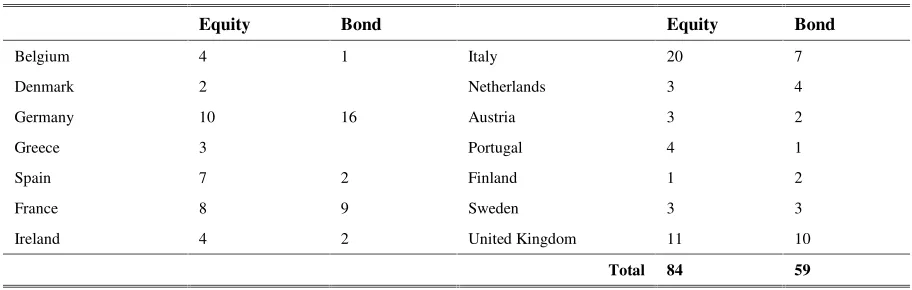
Our data set consists of monthly observations from January 1991 to March 2001. The relatively high frequency of the data highlights one fundamental advantage of market-based indicators relative to balance sheet indicators. We decided to use monthly data, rather than an even higher frequency, in order to eliminate some of the noise in daily equity and bond prices. The data set consists of those EU banks, for which the necessary rating, equity and bond market information is available. In the sample selection process we started from roughly 100 EU banks, which had obtained a “financial strength” rating from Fitch/IBCA.14 The sample size was then largely determined by the availability of market data. The two sub-samples used in evaluating the equity and bond market signals consist of 84 and 59 banks, respectively (see Table 1). The samples contain banks from 14 (equity sample) and 12 (bond sample) EU countries.
III.A Measurement of bank “failures”
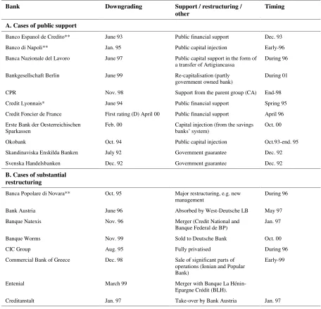
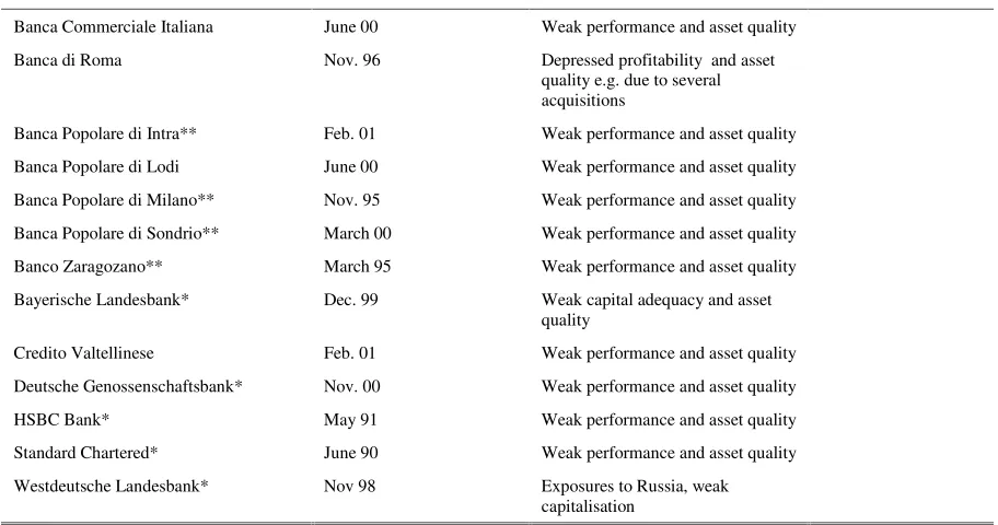
We were faced with the problem that no European banks formally declared bankruptcy during our sample period. In the absence of formal bank defaults, we considered a downgrade in the Fitch/IBCA “financial strength” to C or below as an event of materially weakened financial condition.15 There are 25 such downgrades in the equity and 19 in the bond sub-sample, 32 in total (Table 2). We defend our definition of bank “failure” on two grounds: First, the “financial strength rating” is designed to exclude
14
For an explanation of a “financial strength” rating see below.
15
the safety net and, hence, should indicate the bank’s true financial condition. A downgrade to the level of C or below signifies that there are significant concerns regarding profitability and asset quality, management and earnings prospects. In particular when the rating falls to the D/E category very serious problems are indicated, which either require or are likely to require external support. Second, in many cases after the downgrade to C or below, public support was eventually granted or a major restructuring was carried out to solve the problem. As detailed in Table 2, 11 banks received public support, and 8 banks underwent a major restructuring after the downgrading. The support or restructuring operations also generally took place relatively soon after these events (6-12 months). In the remaining cases, no public support or substantial restructuring took place. In part this is a reflection of sample truncation in March of 2001, as 6 of the remaining 13 downgrades took place in late 2000 or early 2001 and an eventual intervention cannot be excluded. Given that the downgrades precede the actions aimed at resolving the problem by quite some time, we would argue that our proxy for bank failures is quite sensible and generally should bias our results against finding predictive power of the indicators.
Our study is similar to the US studies investigating the relationship between market information and supervisory ratings (for example Evanoff and Wall 2000b, DeYoung et. al. 2000, and Berger et. al. 2000), while we use the “individual” ratings as signals of banking problems. While we are concerned about our relatively small sample sizes (at least in terms of number of banks, not in terms of data points; see below) Evanoff and Wall (2000b), for example, consider 13 downgrades in supervisory CAMEL ratings in a sample of 557 US banks, constituting the default events. Hence, compared to the previous literature our sample appears reasonably large and fairly balanced. Further, rather than use the Fitch/IBCA ratings, it could be argued that we should use supervisory ratings (such as CAMEL ratings) instead. Unfortunately, we did not have access to historical supervisory information on individual banks and, in some European countries, comparable ratings by supervisors do not exist. Clearly, the supervisory ratings may be based on more detailed information relative to ratings by a ratings agency, including confidential information obtained at on-site inspections, but they may also be subject to forbearance.
III.B Market indicators
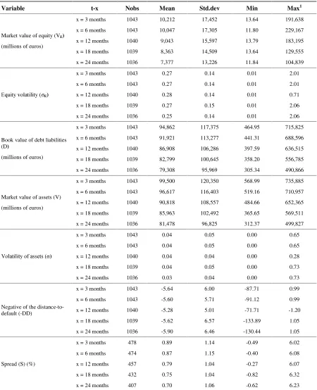
We calculated the negative of the distance-to-default (-DD) for each bank in the sample and for each time period (t) (i.e. month) using that period’s equity market data.The system of equations in (2) was solved by using the generalised reduced gradient method to yield the values for VA and σA, entering
into the calculation of (-DD). Variable definitions are given in Table 3 and descriptive statistics in Table 4.
As to the inputs to the calculation of (-DD), we used monthly averages of the equity market capitalisation (VE) from Datastream. The equity volatility (σE) was estimated as the standard deviation of
(as e.g. in Marcus and Shaked 1984). The presumption is that the market participants do not use the very volatile short-term estimates, but more smoothed volatility measures. This is not an efficient procedure as it imposes the volatility to be constant (it is stochastic in Merton’s original model). However, equity volatility is accurately estimated for a specific time interval, as long as leverage does not change substantially over that period (see for example Bongini et. al. 2001). The total debt liabilities (VL) are
obtained from published accounts and are interpolated (using a cubic spline) to yield monthly observations. The time to the maturing of the debt (T) was set to one year, which is the common benchmark assumption without particular information about the maturity structure. Finally, we used the government bond rates as the risk-free rates (r).16 The values solved for V and σ were not sensitive to changes in the starting values.
We largely followed convention when calculating the monthly averages of the secondary market subordinated debt spreads (S). We used secondary market spreads, rather than those from the primary market, as we would argue that secondary market spreads are more useful for the ongoing monitoring of bank fragility. In the absence of mandatory issuance requirements, such as those proposed by Calomiris (e.g. 1997), banks’ new issuance could be too infrequent, or limited to periods when pricing is relatively advantageous. As we were concerned about too thin or illiquid bank bond markets in Europe, we only selected bonds with an issue size of more than euro 150 million. This figure seemed the best compromise between maintaining sample size and obtaining meaningful monthly price series from Bloomberg and Datastream, which were our main data sources. In addition, in order to minimise noise in the data series, we attempted to use fixed rate, straight, subordinated debt issues only. We were largely able to obtain such bonds, but in some cases we had to permit floating rate bonds into the sample. We used the standard Newton iterative method to calculate the bond yields to maturity.
For the larger countries, we were able to find bank bonds issued in the domestic currency, which met our liquidity requirement. In case of smaller countries, banks more frequently issued foreign than domestic currency-denominated bonds prior to the introduction of the euro. Hence, we largely resorted to foreign currency issues (DM, euro, USD and in two cases, yen) and matched them to government bonds issued in the same currency. We were able to construct risk-free yield-curves for Germany, France and the UK and calculated spreads for banks in those countries relative to the corresponding point on those curves. For the other smaller countries, we were unable to obtain sufficient data to construct full risk-free yield-curves. We therefore instead matched the remaining term to maturity and the coupon of the bank bond to a government bond issued by the government of the country of the bank’s incorporation in the same currency.
16
III.C Expectation of public support
We use the “support rating” issued by Fitch/IBCA to indicate the likelihood of public support. We regard as cases of more likely public support the rating-grades 1 or 2 (see Appendix 2). The former grade indicates existence of an assured legal guarantee, and the latter a bank, for which in Fitch/IBCA’s opinion state support would be forthcoming. This could be, for example, because of the bank’s importance for the economy. Hence, the likelihood of support could depend on the size of the institution (“too-big-to-fail”), but a bank could be possibly “systemically” important also for other reasons. The weaker “support ratings” (from 3 to 5) depend on the likelihood of private support from the parent organisation or owners, rather than from public sources.The share of banks with a “support rating” of 1 or 2 is quite high (around 65% in the equity sample and 80% in the bond sample). This is not surprising, since we are considering banks with a material securities market presence as an issuer. These banks tend to be significantly larger, again as expected, than those with a rating of 3 to 5. Their average amount of total debt liabilities is roughly 10 times higher.
III.D Sample Selection
Before we present the results, it may be worthwhile to examine the sample in a little more detail, in particular with respect to sample selection issues. The first question that arises relates to the relevant universe of banks. For the bond sample, the universe is determined by those banks in the EU that were rated by Fitch/IBCA during the ten-year period under investigation.17 Out of this total, those banks remained in the sample, for which we were able to calculate bond spreads, i.e. for which sufficiently liquid and sizeable bonds were outstanding and the data were available in Bloomberg. Hence, relative to the universe of 103 rated banks, we were able to obtain meaningful bond price data for 59 banks. Sample selection issues may be a problem, if the banks in sample differ in their likelihood of failure relative to those in the universe of banks. In particular, we were concerned that we had tended to over-sample failures. It turns out that this is not the case. The probability of failure during the sample period is around 33 percent both in the universe and in the sample. Nevertheless, the banks in the sample may differ in other important criteria from those in the universe. For example, given our requirement that the bank must have substantial subordinated debt outstanding, the banks in the sample may be larger than those in the universe. This is the case, although the difference is not statistically significant.Finally, a bias may arise due to differences in data availability of the banks in the sample. If banks that eventually fail remain in the sample only a relatively short period of time prior to failure, the proportional hazard model may overstate the predictive power of indicators. There could be a number of reasons for this problem. One,
17 Clearly, this universe is substantially different from the notion of all EU banks. For small, non-traded banks,
given that we chose a fixed starting point for our sample (1991) and given that naturally all failed banks drop out after failure, the time period that non-failed banks remain in the sample is longer. This by itself should not constitute a problem for the estimation. However, if failures occur disproportionately at the beginning of the sample period, i.e. in 1991-1994, this could result in overstating the predictive power of our indicators in the proportional hazard model. However, the average time period in the sample for banks, which eventually failed, is 34 months. This should give us ample data to obtain unbiased estimates.18
In case of the stock price sample, we would argue that the relevant universe is somewhat smaller. Again taking those banks, which had obtained a rating from Fitch/IBCA as the starting point, the universe of banks is further reduced by banks, which are not listed at a major European stock exchange. It turns out that this concerns 11 banks. Of the remaining 92 banks, our sample contains 83 banks. The difference of nine banks is due to the unavailability of a stock price series in Datastream. The probability of failure in the sample is identical to that in the universe at one third. Again, we were concerned whether we observe the failing banks long enough to make meaningful inferences from the proportional hazard model. The average time of banks, which eventually fail, in the stock price sample is one month longer than those in the bond price sample, namely 35 months (non-failing banks: 73 months). Again, we feel that this should give us sufficient data to estimate the model.
IV. Descriptive statistics
We constructed the sample for the empirical analysis as follows. For each month (t) of a downgrading (“default”) event, we took all non-downgraded banks as a control sub-sample, and calculated all variables for both sub-samples with specified leads of x months.
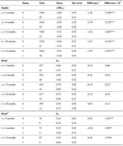
As a first cut at the data, we conducted simple mean comparison tests to assess whether (-DD) and S are able to distinguish weaker banks within our data set. We also examined whether the indicators could lead the downgrading events by performing the mean comparison tests for various time leads (lead times of 3, 6, 12, 18 and 24 months). The results reported in Table 5 indicate that the banks that were downgraded had a significantly higher mean value of (-DD) than the non-downgraded banks up to and including 24 months prior to the downgrading events. We also find in the second panel that the banks that were downgraded had higher prior spreads (S) and that the spreads of the “defaulted” banks clearly increase as the “default” event is approached. However, the difference between “defaulted” and “non-defaulted” banks is never statistically significant when the full sample is considered. This suggests that S is a weaker leading indicator of bank fragility than (-DD).
18
The “default” indicators reflect two factors: One, the bank’s ability to repay out of its own resources, and, second, the government’s perceived willingness to absorb default losses on behalf of private creditors (e.g. Flannery and Sorescu 1996). Hence, in the third panel of Table 5 we limit the sample to those banks with a support rating of 3 or higher. We only present the t-tests up to x equal 12 months in order to maintain some sample size. Nevertheless, the figures given here should be interpreted with care, as even so sample sizes are small. The results offer further evidence that a safety net expectation can dilute the power of the spreads to reflect bank fragility, while there is no apparent impact on the distances-to-default. In this limited sample, there is now a significant difference in the mean values of S between “defaulted” and “non-defaulted” banks. Also in absolute terms, the difference in the average spreads is now higher.
V. Empirical estimation
V.A Estimation methods
We used two different econometric models to investigate the signalling properties of the market-based indicators of bank fragility. The first is a standard logit-model of the form:
) DI * DSUPP DI
( ] 1 STATUS
Pr[ t = =ψ α0+α1 t−x+α2 t−x t−x (7)
where ψ( ) represents the cumulative logistic distribution, DIt-x the fragility indicator at time t-x, and
=
otherwise 0
t time at below or C to downgraded was
bank if 1
STATUSt .
We estimate the model for different horizons separately, i.e. we investigate the predictive power of our two indicators 3, 6, 12, 18 and 24 months before the downgrading event. Generally, we would expect the predictive power to diminish as we move further away from the event. Significant and positive coefficients of the lagged market indicators (indicating a higher unconditional likelihood of problems when the fragility indicators have a high value) would support the use of (-DD) or S as early indicators of bank fragility (Proposition 1).
banks, while they are independent across banks. Therefore, we adjusted the standard errors using the generalised method based on Huber (1967).
Our second model is a Cox proportional hazard model of the form:
X 2 DI 1 0(t)e
h ) X , DI , t (
h = β +Β , (8)
where h(t,DI,X) represents the proportional hazard function, h0(t) the baseline hazard, and X some control variables (see below). Again, we calculated robust standard errors, as we had multiple observations per bank and used Lin and Wei’s (1989) adjustment to allow for correlation of the residuals within banks. The model parameters were estimated by maximising the partial log-likelihood function
(
)
∑ ∑ +Β
−
∑ +Β
=
= ∈ ∈
D
1
j r Dj 1 r 2 r j i Rj 1 i 2 i
) X DI exp( ln d X DI L
ln β β , (9)
where j indexes the ordered failure times t(j) (j=1,2,…D). Dj is the set of dj observations that
“default” at t(j) and Rj is the set of observations that are at risk at time t(j). The model allows for
censoring in the sense that, clearly, not all banks “default” during the sample period.19
The two models provide a robustness check whether equity and bond market indicators have signalling property as regards bank “defaults”. In addition, they also provide insights into two distinct questions: The logit-model permits a test of the unconditional predictive power of the indicators with different lead-times, whereas the proportional hazard model yields estimates of the impact of the market indicators on the conditional probability of “defaulting”. The latter means that we obtain “default” probabilities, conditional on surviving to a certain point in time and facing a certain (-DD) or S in the previous period.
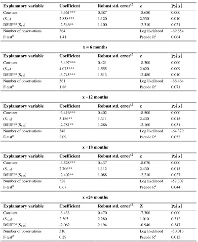
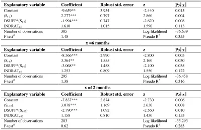
V.B Logit-estimation results
Table 6.A reports the results from estimating logit-models with different time-leads. An increased (-DD) value tends to predict a greater likelihood of financial trouble. The respective coefficient is significant at the 10%-level for the 6, 12 and 18-month leads. Hence, we find support for Proposition 1: (-DD) appears to have predictive properties of an increased (unconditional) likelihood of bank problems up to 18 months in advance. The coefficient ceases to be significant more than 18 months ahead of the event. However, we found the insignificance of the coefficient of the 3-month lead somewhat puzzling. We suspect that the reason is increased noise in the -DD measure closer to the default, as evidenced by
19
the higher standard error for the 3 than the 6-month leads. It may be the case that many eventually downgraded banks exhibit a lowering in the equity volatility just before the downgrading, which causes the derived asset volatility measure to decrease as well, reducing the (-DD) value.
Turning back to Table 6.A., we find that the coefficient of DSUPP*(-DDt-x), measuring the impact
of the safety net, is never statistically significant. Moreover, the hypothesis that the coefficient of (-DDt-x)
is zero for the banks with a strong expectation of government support is rejected for all lead times, except for x=24. The safety net does not appear to be important for the predictive power of the distance to default as an indicator of bank fragility.
The results for the bond spreads, S, strongly support Proposition 1 as well (see Table 6.B). The coefficients for lead times of up to 18 months are significant at least at the five percent level. The results also highlight that it is important to control for the expectation of public support in case of spreads. The coefficient of the interacted term (DSUPP*St-x) is significant and negative, and, a joint hypothesis test
reveals that the coefficient on the spread is zero for the banks with a high (a rating of 1 or 2) expectation of public support. This finding is in contrast to the results using -DD as an indicator of bank fragility.
A convenient way to summarise the results of the logit models just described is given in Chart 3. The chart presents the coefficients from Tables 6.A and 6.B, normalised, such that the maximum effect is equal to one. It reveals that the maximal predictive power of spreads occurs quite shortly before default, around 6 to 12 months before. In contrast, DD has relatively little predictive power close to the event, but instead reaches its maximum no less than 18 months ahead of the default. These patterns correspond closely to the theoretical predictions of the option pricing framework discussed in section II.
The results of discrete choice models may be quite sensitive to the underlying distributional assumptions, in particular in cases where the distribution of the dependent variable is as skewed as in this sample. Only four percent of the bond sample and three percent of the stock sample were “defaulting” observations. As a simple robustness check, we estimated the corresponding Probit-models and found essentially unchanged results, both in terms of magnitude and significance.20
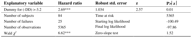
V.C Hazard-estimation results
Tables 7 and 8 give the hazard ratios and corresponding P-values for a model without additional control variables for both (-DD) and S. Only (-DD) is significant (at the 5% level); both indicators have the expected positive signs. The hazard ratios, indicating a greater conditional likelihood of “default”, are increasing in the values of the fragility indicators, which is consistent with the logit-results.
20
The tables also show the results for a test of the proportional hazard assumption (i.e. the zero-slope test), which amounts to testing, whether the null hypothesis of a constant log hazard-function over time holds for the individual covariates as well as globally. For (-DD), this assumption is violated. Hence, we present in Table 9 results from an alternative model specification, in which we use a dummy variable of the following form
− >−
=
otherwise 0
2 . 3 ) DD ( if 1
ddind , (10)
where –3.2 represents 25th percentile of the distribution of (-DD). Hence, in this specification, we investigate whether banks with “short” distances to default are more likely to fail compared to all other banks. We find that the indicator significantly (at the 1%-level) increases the hazard of a bank “defaulting”, as before, and the model is no longer rejected due to the violation of the proportional hazard assumption.
We also examined the weaker performance of S than -DD in the baseline specification (as given in Tables 7 and 8). In the logit-model, we found that two factors significantly affect the predictive power of the spread: the presence of a safety net and whether or not the bank resides in the UK. Table 10 shows that the coefficient of the spread significantly improves when controlling for the UK by means of a dummy variable. S now is significant at the 1%-level. In addition, the dummy for the UK is significant at the 5%-level: higher spreads in the UK are associated with a significantly lower hazard ratio, i.e. a significantly lower likelihood of failure. For -DD the inclusion of the safety net dummy or the UK dummy do not materially affect the results, as in the logit-specification, and are not reported here. Further, the logit results suggested that for banks, which are likely to benefit from public support in case of trouble, the predictive power of bond spreads is reduced to zero. This finding is confirmed in Table 11.
not explore this issue further. We only conclude that a UK spread puzzle remains, which we cannot explain.21
Even more interesting, we can immediately read off the difference in the survivor probability, given that a bank has remained in one or the other group. For (-DD), we find no difference in the hazard even after 2 years (24 months). Differences only arise subsequently: after 36 months, a bank which had a (-DD) > -3.2 for that period of time has a failure probability that is 20 percentage points higher relative to a bank that was consistently in the control group. This is consistent with the findings in the logit-model: (-DD) is found to be an indicator, which has better leading properties for events further in the future. In contrast, spreads react only relatively shortly before default. Given survival, spreads essentially lose all their discriminating power after one year. The results also highlight that the prevalence of indicators matters, which suggests that the use of hazard-models add new insights relative to standard logit-models. Logit-models are unable to yield predictions, which are conditional on default indicators having prevailed for periods of time.
Hence, in line with Proposition 2, the spread reacts more closely to the “default” point than (-DD). Put differently, banks may “survive” substantially longer with a short distance-to-default, but the likelihood of quite immediate problems is very high, if they exhibit a high spread (in our definition of 100 basis points or above). As we show in the earlier part of this paper, the strong reaction of the spreads only close to the default point is explained by the non-linear pay-off profile of subordinated debt-holders.
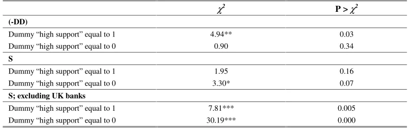
Finally we present log-rank tests of the equality of survivor functions for those banks with an implicit safety net (“support rating” of 1 or 2) in Table 12. We find that the distance to default has more predictive power for banks, which are likely to benefit from governmental support, and little predictive power for those that do not.22 More importantly, Table 12 shows the importance of UK banks, as well as the safety net for the predictive qualities of bond spreads. With UK banks included, we find only weak discriminating power of spreads even for banks, which are not likely to receive public support in case of problems. Without UK banks, however, we find that spreads perform significantly better in case of banks with little or no public support, confirming our earlier results and Proposition 3.
21
Gropp and Olters [2001] attempt an explanation using a political economy model. They argue that as the UK has a market based financial system as opposed to continental Europe, which is bank based, a political majority to bail out banks is more difficult to obtain in the UK. Investors, therefore, want to be compensated for this additional default risk and require higher spreads.
22
VI. Robustness and extensions
As an extension, it is interesting to examine whether the market indicators contain information, which is not already summarised in ratings. To this end, we controlled for the “individual rating” at the time the market indicators were observed. The results given in Table 13.A for the (-DD) measure are fairly similar to those reported in Table 7.A, albeit the significance of the (-DD) indicator is somewhat reduced. Overall, they suggest that the (-DD) indicator adds to the information obtainable from (Fitch/IBCA) ratings and the more the longer the time leads. The results are even stronger for the spreads (see Table 13.B). We conclude that both of the indicators analysed in this paper appear to contain additional information from ratings, at least in terms of their ability to predict bank “failures”.
This also addresses the specific issue raised by our definition of “failures”. Namely, there is the possibility that we would be using market indicators to predict rating down-gradings, which could be based on the same set of information of the probability of default. However, as we find that the market indicators contain additional information compared to prevailing ratings, this concern does not seem to be warranted. However, even if the ratings would contain completely similar information as our market indicators, we would find support in our standard logit and hazard models to using market indicators: high-frequency market data has leading properties over discrete bank problem events reflected in their individual ratings.
We also checked whether the distance-to-default measure performs better in terms of its (unconditional) predictive property than simpler equity-based indicators. First, we estimated the logit-models using the equity volatility as the fragility indicator. It, however, turned out to be a significantly weaker predictor of “default”. The coefficients of σE,t-x were never statistically significant. The composite
nature of the (-DD) apparently improves predictive performance and reduces noise. We found similar results for a simple leverage measure (VE/ VL).23
Next, we wanted to explore whether our market indicators add information to that already available from banks’ balance sheet. Conceptually, this is obvious: Market based indicators should fully reflect past balance sheet information as well as forward looking expectations about the prospect of the bank. First note that we were unable to estimate the hazard model with balance sheet variables, as they fail to be available at a monthly frequency. Hence, we estimated logit models only.24 Clearly, the choice of which balance sheet variables to use is arbitrary. We followed the previous literature (see e.g. Sironi (2000), Flannery and Sorescu (1996)) and considered a set of balance sheet indicators emulating the categories of
23
The results are available from the authors upon request.
24
CAMEL ratings (Capital adequacy, Asset quality, Management, Earnings, Liquidity).25 Then, we calculated a composite score based on the bank’s position in each year’s distribution for every indicator.26 In this way, we were able to consider the correlation between the different indicators, i.e. whether a bank is “strong” or “weak” by more than one indicator. In order to ensure comparability, we re-estimated the model containing only the market indicators, in order to ensure comparability given the reduced sample size. Second we estimated a model only with balance sheet indicators and third a model combining market and balance sheet indicators. Here, we only report results for the 12 months time lead.
Results for the distance-to-default indicator (Table 14.A), show that it adds some information to that already available from balance sheet data. In the model combining the distance-to-default and the balance sheet indicators, the distance-to-default indicator is significant (at 5% level), and the model fit, as measured by the pseudo-R2 increases from 0.20 to 0.24 over the one containing only balance sheet variables.27 In addition, the significance of distance to the default indicator improves in the combined model, when compared with the model with only the distance-to-default indicator. This suggests that the distance-to-default indicator provides additional information to that of balance sheet variables, but it does not replace the balance sheet indicators. In other words, the distance-to-default and the balance sheet indicators are both useful for the monitoring of banks and play a complementary role.
Empirical estimates from the same exercise for the spreads indicator are presented in table 14.B. They suggest that spreads also add some information to that already available from balance sheet data, although the evidence is weaker. As before, the model combining the spreads and the balance sheet indicators has a slightly better fit (in terms of pseudo-R2) over the one containing only balance sheet variables. However, by itself spreads are not significant, even for the banks that are not expected to be supported. Our interpretation is that spreads are highly correlated with the balance sheet information and, hence, to some extent simply appear to reflect backward looking information, rather than information about the future performance of the bank.
Clearly, tests of the sort presented here have the drawback that they can always be criticised on the basis of omitted variable bias, i.e. that some other balance sheet indicator may be more relevant. In order
25 In order to maintain a sufficient sample size in the set of failed banks, we had to consider only four out of five indicators.
Hence, the liquidity indicator was taken out from the analysis.
26 The composite score is calculated in the following way:
• We considered the percentile ranking of the bank in each year distribution for every indicator;
• We divided the ranking distributions in four quartiles, and assigned a score varying from 0 (best) to 3 (worst) to the position of the bank in the rankings;
• We obtained the composite score simply summing up the scores for each indicator, yielding a variable ranging from zero (a bank in good condition with all indicators) to 15 (a bank in bad condition with all indicators).
The FDIC uses a broadly similar approach for its CAMEL model (see FDIC (1994)).
27
to alleviate this criticism, we have taken care to use variables in line with the previous literature and have also tried to emulate a CAMEL approach, which is used by many regulators. The most important result based on this exercise may be that we find some complementarity between market and balance sheet indicators.
Finally, we wondered whether the two market indicators might not provide complementary information to each other. In particular, in the previous section, we demonstrated that the two indicators have very different predictive properties through time. Spreads react late, but lose predictive power further away from the event. The distance to default is not a very strong indicator close to default, but has strong leading properties around two years out.28 Table 15 gives the results from a model with both indicators included simultaneously. We find that both variables are significant at least at the 5 percent level.
Based on this finding, we can ask two further questions. One, which combination of spread and distance to default gives us the most discriminatory power? And, second, is this an improvement over using one or the other indicator alone? In Chart 5 we attempt to shed some light on both questions. In the top panel we have given the survivor functions for banks, which are above the median in at least one of the indicators and are in the top 75th percentile in the other versus all other banks. We find that the survivor functions are not significantly different from one another. In the bottom panel, we have plotted the survivor functions for banks that are above the median in both indicators versus all other banks. Now the survivor functions are statistically significantly different at the 5 percent level. It turns out that the “above median in both indicators” criterion gives us maximal discriminatory power.
Further, comparing the lower panel of Chart 5 to Chart 4, we find that the combination of both indicators provides us with better discriminatory power than either indicator alone. In comparison to the distance to default (top panel of Chart 4), we have significantly more discriminatory power closer to the default, which we would attribute to the addition of information contained in spreads. Looking at the lower panel of Chart 4, we find that the addition of information contained in the distance to default to spreads, reduces type one error dramatically. We are missing significantly fewer defaults, when using a combination of both indicators, which is evident from the much flatter curvature of the top line in Chart 5 compared to Chart 4 (lower panel). Overall, we conclude that the market indicators appear to provide useful information not only relative to balance sheet information and ratings, but also to each other.
28