The Ex Ante Predictive Accuracy of Alternative Models of the Term Structure of Interest Rates

(1)

Abstract

Basma Bekdache

Wayne State University

Christopher F. Baum

Boston College

August 19, 1997

The Ex Ante Predictive Accuracy of

Alternative Models

of the Term Structure of Interest Rates

We acknowledge suggestions offered by Christian Gilles, Robert Bliss, and participants in the Third Annual Conference of the Society for Computational Economics, June 1997. The standard disclaimer applies. Please address correspondence to Bekdache, FAB 2101, Dept of Economics, Wayne State University, Detroit, MI 48202; phone: 313.577.3231, fax: 313.577.0149, email: [email protected]

This paper compares six term structure estimation methods in terms of actual ex ante price and yield prediction accuracy. Specically, we examine the models ability to price Treasuries for one to ve trading days ahead. The models performance differs markedly between in- and out-of-sample predictions. Their relative success also depends on time, the forecast hori-zon, and whether price or yield errors are compared. We examine the degree of loss in accuracy the modeler incurs by not using the best method: in particular, we compare the more complex splining methods and the par-simonious Nelson-Siegel model.

Keywords: term structure, ex ante forecasts, spline models, Nelson-Siegel approach

(2)

1

1. Introduction

The split-sample approach may be employed for a purely econometric rationale, such as determining whether a method is overtting the in-sample data.

Modeling the term structure of interest rates has been the subject of a vast literature in economics and nance. Characterizing interest rates as a function of maturity embodies information about future movements in interest rates and has direct implications for real economic activity. In nancial markets, the term structure is crucial to the pricing of interest-rate-contingent claims and xed-income derivative securities. Although many analytical interest rate models imply particular shapes for the term structure, much of the empirical literature has been concerned with tting model parameters to the data in order to faith-fully reect the interrelations among observed prices and yields. A wide gulf exists between the specic predictions of theory and the complex empirically derived forms of many term structure estimation models.

(3)

shifts during the forecast period, confounding identication of prediction errors; but in a very liquid market, the shifts are in the nature of common factors, affecting all similar bonds in a common fashion. Our approach to these issues focuses more sharply on how we might reasonably compare these competing methodologies, using measures of ex ante predictive accuracy, than on the spe-cic scores attained by each model, or the uncertainty generated by the forecast horizon.

The purpose of this study is to apply ex ante measures of predictive accuracy to six term structure estimation methods and evaluate their relative performance over quarter-end dates for a six-year period. These methods can be considered partial equilibrium, or no-arbitrage approaches to the term structure, in that the no-arbitrage condition is used to empirically determine the shape of the term structure from price and yield data on individual securities. Five of the six methods utilize cubic splines to approximate the term structure, differing in the choice of function which is splined and the degree to which the parameterization is determined by the data. The sixth method is the well-known Nelson-Siegel approach, in which the yield curve is derived from a second-order differential equation applied to Treasury coupon STRIPS data. The spline methods are applied to essentially all of the Treasury (bill, note, and bond) issues, so that their performance approximates that achievable by a practitioner with access to the entire Treasury curve. We analyze the models performance on the quote date and for each of the following ve trading days, and generate an array of parametric and non-parametric summary measures on the modelsp erformance by date, by tenor of security, and by length of forecasting horizon.

(4)

d

( ) =

( )

P t T t

P t

r

2. Survey of the Literature

2.1. Notation and Basic Framework

generate the best yield forecasts. Several methods show marked differences in their ability to generate accurate forecasts when the horizon of the forecast is varied from one to ve trading days. There is considerable time variation in the relative performance of the models considered; although one of the spline models stands out, it dominates the other models in fewer than half of the cases, and is often dominated by the parsimonious Nelson-Siegel approach. The correlations between models forecasts and movements in the yield curve are low at long horizons; this suggests that the models relative performance is not strongly af-fected by shifts in the yield curve. A general statement on the superiority of any of these competing models would not be justied as their relative performance is quite sensitive to the level of rates, to the forecast horizon, and to the tenor of the underlying securities.

The plan of the paper is as follows. Section 2 surveys the literature. In subsection 2.1 some basic notation and terminology are introduced followed by a brief description of the various no-arbitrage methodologies in subsection 2.2. Section 3 presents the data and estimation methods to be compared. The in-and out-of-sample evaluation of the methods, over the full sample in-and tenor subsamples, is presented in section 4. Finally, we summarize the results and make concluding remarks in section 5.

(5)

d X =1 2 3 2 3 0

0 0 0

0 0

0

f ( ) = dlog(P /d .( ))

d d

d d d

d d d d th i n j

i d d

i i

d

( ) exp( ( )) = 1

( ) = log( ( )) ( )

( )

( ) = log( ( ) ( )) ( )

( )

=

( ) = ( + ) ( + ) + ( )

( ) ( + )

+ = 2

( )

P r .

r P / P

r

t T t

f t, t , T P t, T /P t, t / T t .

P t, t t t

t < t < T

t T t

P C t j P t j P ,

P C t j

t j n

P

Assuming that the discount function is differentiable, the instantaneous forward rate is computed as:

(2.2)

Cox, Ingersoll and Ross (CIR hereafter) (1985a, 1985b) developed the rst general equilib-rium model of the term structure of interest rates. Prior attempts to model the term structure in a partial equilibrium setting include Vasicek (1977) and Brennan and Schwartz (1979).

(2.1) Alternatively, is the rate of growth of , or the yield to maturity. The term structure of interest rates is the function relating the -period spot rate, , to . In addition to the discount and spot rate functions, the term structure can also be represented with forward rates, which are essentially implicit future spot rates. The forward rate for the time interval

to observed at is given by :

(2.3) Where denotes the time price of a discount bond maturing at time and . In the absence of arbitrage opportunities, the value of the i coupon bond at time , maturing in periods, equals the sum of the present values of its stream of cash ows,

(2.4) where denotes the theoretical price of the bond and denotes the bonds promised cash ow at time . is the number of semiannual coupon payments over the life of the bond.

(6)

Alterna-4

4

X

=1

d

i

n

j

i d d i

i P

P C t j P t j P .

( )

( ) = ( + ) ( + ) + ( ) +

2.2. No-Arbitrage Methodologies

2.2.1. McCullochs Splining Method

Methods which were used prior to McCullochs papers include Durands hand tting yield curve technique and the point-to-point or bootstrap method (e.g. Carleton and Cooper (1976)). Since none of these techniques are directly relevant to the current literature, we con-centrate on studies following McCulloch (1971, 1975).

tively, the no-arbitrage approaches generally t observed bond prices to the pricing constraint in (2.4) to estimate the parameters of a given function (the discount, forward rate or the spot rate function) that relates interest rates to term-to-maturity. We now turn attention to a more detailed description of the various no-arbitrage approaches to term structure modeling.

The main focus of this second branch of the literature is to use the no-arbitrage condition in (2.4) to nd a functional form that can best approximate the term structure. McCulloch (1971, 1975) introduced the practice of using approximat-ing functions such as polynomials and splines to empirically approximate the discount function . Since these papers, various approximating functions have been proposed to t either the discount function or one of its variants. In this section we discuss only those methods which we implement in this study.

Recall the bond price equation from (2.4)

(7)

0

(

5

d

j j j

j

th

i i

j i

i

i ia ib ia ib

0 1 2 2 3 3 4 13 5 23 6 33

0 0 1 1 2 2 3 3 4 1 5 2 6 3

0

( )

( ) = + + + + + + +

= :

0 :

=

( ) = + + + + + + + +

( + )

= ( ) 2 +

This discussion of McCullochs cubic spline is based on Baum and Thies (1992). P

P

P b b b b b z b z b z ,

z k > k

k ,

b .

P b X b X b X b X b K b K b K .

X C t j

K X s b

v P P / b P P b

In McCullochs methodology, the discount function, , takes the form of a cubic spline. This means that if we divide the maturity spectrum into a number of intervals, is a different third-order polynomial over each interval. These piece-wise polynomials are joined at knots or break points so that the splines rst and second derivatives are set equal at those points. A parameterized representation of this approximation is given by

(2.6)

where

the knot points of the spline

the parameters of the estimated discount function Substitute (2.6) into (2.5), then the price of the i bond is

(2.7) In (2.7), the are functions of the cash ows and of term to maturity

(8)

6

( )

j

d

k

P

2.2.2. Fisher et al.: Smoothing Splines

In Fisher et al.s study, the discount function is parameterized using a Basis Spline (B-spline) rather than using independent parameters as shown in (2.6). The properties of B-splines (see de Boor (1978) for details) provide for the efficient and numerically stable calculation of spline functions. A cubic spline which is formed as a linear combination of B-splines can be easily evaluated and manipulated.

bid price and brokerage fees, respectively. This adjustment prevents the esti-mates from being affected by large errors that are caused solely by transactions costs. McCulloch chooses the knots such that there is an equal number of bonds in each interval. Estimating the discount function as a cubic spline allows for greater exibility in approximating complex shapes since the parameters of the curve in a given interval are heavily inuenced by observations in that in-terval. However, this exibility can sometimes result in curve shapes that seem unreasonable, such as the negative forward rates in McCullochs paper. Shea (1984) discusses placing constraints on the spline and varying the number and placement of break points as potential solutions to these problems.

(9)

00 X Z P P =1 2 0 =1 2 2 =1

( )2 ( )

N i i T d d d N i i n N N i i i i i d d + ( ) ( )

( ) = 0

( )

( ) = 1 ( )

(1 )

( )

(1 )

( ) log ( ) ( )

P d ,

N P P GCV GCV N , n GCV CV

/N i

i

CV

P P f

(2.8) where is the number of bonds in the sample. The second term in (2.8) measures the non-smoothness in the approximating function as it will be larger the greater the variation (wiggliness) in . Note that if , a knot will be placed at each observation, as this achieves a perfect t. Thus in choosing the optimal number of knots, the t as measured by the least squares term is balanced against smoothness according to , the weight given to the non-smoothness term. In this method, is chosen to minimize the Generalized Cross Validation criterion

(2.9) where is the number of parameters of the spline. Craven and Wahba (1979) developed the approach as an approximation to the Cross-Validation score with equal to the residual for the th observation obtained from estimates of the model with the th observation omitted from the sample. The process of omitting an observation and predicting it using the remaining observations is repeated for all data points to generate the average residuals of the omitted observations given by the score. Choosing the optimal smoothness parameter by minimizing (2.9 ) and essentially simulating true out-of-sample prediction errors amounts to limiting the inuence of each data point in determining the variability in the tted curve.

(10)

d

0 1 2

0 1 2 2

2.2.3. Nelson-Siegel: A more parsimonious approach

f / / / .

r / / / / .

r a b / / / c / .

r

a b c

( ) = + exp( ) + [ exp( )]

0

( ) = + ( + )[1 exp( )] ( ) exp( )

( ) = + [1 exp( )] ( ) + exp( ) +

( )

evaluate the ability of each method to produce stable and reasonable estimates of the forward and discount functions. Their ndings indicate that splining the forward rate function with GCV produces the best overall results.

In the Nelson and Siegel (1987) (NS hereafter) approach, the relationship be-tween yield and maturity is derived from the assumption that spot rates follow a second-order differential equation and that forward rates, being forecasts of the spot rates, are the solution to this equation with equal roots. Thus we have (2.10) By integrating (2.10) from to , we get the yield to maturity or discount rate function

(2.11) Following NS, we parameterize (2.11) in order to t the yield curves. The equation to be estimated is given by

(11)

7 7

3.1. The Data

Wall Street Journal

Journal

3. Data and Estimation Methods

Bliss approach also takes the recorded bid and ask prices into account; in his treatment, predicted prices within the observed bid-ask spread are considered to have zero prediction errors. The method has been used in a slightly different manner by Baum and Thies (1992) in that they apply it to smooth or post-lter their cubic spline term structure estimates, obtained from applying McCullochs methodology to U.S. railroad bond quotations. In a recent paper, Bliss (1997) applies an extended form of the Nelson-Siegel approximating function (2.11) directly to Treasury bond prices. In this context, the estimation problem is rendered highly nonlinear by the inclusion of all of the securitys cashows in a single observation of the dataset. In contrast, the use of Treasury STRIPS, each with a single cashow, greatly simplies the estimation problem.

In this section, we briey describe the data and outline the estimation methods which will be compared in the empirical analysis of the next section. We do not present the estimation results in this paper since our focus is on the forecasting accuracy of the various models. Details on the estimation results are available upon request.

(12)

8

9

8

9

We also estimated the models in this paper with coupon and principal STRIPS. Although the mean forecast errors are larger at all forecast horizons when principal STRIPS are included, our conclusions regarding the relative rankings of the models remain unchanged.

All available quotations on bills, notes and bonds (with the exception of ower bonds) were extracted from the CRSP Daily Government Bond Master dataset. Noncallable securities were agged as such; callable securities priced at a discount to par were given their stated maturity, while (by Street convention) callable securities priced at a premium were given their next call date as their maturity. Our analyses can readily be executed omitting all callable securities.

period, we have chosen to exclude them from the analysis on the advice of practitioners. Many of the heavily traded strippable Treasuries are on special, implying that they may be used as specic collateral in repurchase agreements (RPs) at an RP rate signicantly below market rates. This raises the price of such a security above that which would otherwise prevail, by an amount related to the lower future borrowing costs (for details on the workings of this relationship, see Duffie, 1996, pp. 494-496). To link this discrepancy (which has been found to explain a signicant portion of the on-the-run effect) to coupon and principal STRIPS, we need only consider practitionersclaims (e.g. Gilles, 1997) that the specialness of the coupon security is fully embodied in the principal STRIP, rather than allocated evenly throughout the securitys decomposed cash ows. Given the large number of relatively small coupon cash ows, the concentration of specialness in the principal STRIP is surely a reasonable assumption. Restricting our analysis to coupon STRIPS generates a more homogeneous data set for the estimation of the zero-coupon (spot) curve.

(13)

d

10

11

10

11 P

f

P

Mathematica ( )

log

( )

3.2. Splining Methods: Fixed and Endogenous Knots

DF1:

LDFGCV:

FGCV:

DFGCV:

DF2:

We are indebted to Mark Fisher for providing us with his programs to perform the empirical analysis for this section.

See Fisher et al. (1995, 1996) for more details on the implementation of the splining tech-niques using B-Splines.

Following Fisher et al. (1995, 1996), we employ both xed knots as well as adaptive knot placement specications to estimate the following ve models :

The discount function, , is specied as a cubic spline with the number of interior knots set equal to one-third of the number of bonds in the sample.

The of the discount function is modelled as a cubic spline with adaptive parameters chosen with GCV.

The forward rate function, , is modelled as a cubic spline with adaptive parameters chosen with GCV.

The discount function, , is specied as a cubic spline with adaptive parameters chosen with GCV.

The discount function, , is specied as a cubic spline with the number of interior knots set equal to 10.

(14)

X

=0

d

i i

j

i d

d ( )

ˆ = ( ) ( + ) ˆ ( + )

ˆ ( )

r

a b c

P C t j P t j ,

P

3.3. The Nelson-Siegel Estimates

4. Evaluation of Alternative No-Arbitrage models of the

Term Structure

The Nelson-Siegel methodology is applied to data on U.S. Treasury coupon STRIPS to obtain estimates of the term structure from the approximating func-tion (2.12) on the 26 quarter-end dates between June 1989 and September 1995. is calculated from the average of the quoted bid and ask prices as the continuously compounded yield from settlement to maturity date annualized to a 365-day year. In our implementation, is the number of years to maturity. Following NS, we search over a grid of values for to obtain the best tting values for , and and .

The no-arbitrage approaches differ in two main respects: rst, in terms of the functional form tted to the bond price data, and second, with respect to the criterion function to be minimized to obtain the parameter estimates. In this section, we assess the performance of the various treatments of these aspects cross-sectionally as well as over time in terms of in- and out-of-sample price and yield errors. We concentrate our attention on out-of-sample performance, given the focus of this study. Although the out-of-sample errors include the effects of day-to-day shifts of the yield curve, the comparisons of methods performance on this basis is a more realistic evaluation of their varying abilities.

The price error for each bond is calculated from (2.5) as:

(4.1)

(15)

12

d d

P ˆ ( ) r ˆ ( )

4.1. Price Errors

We focus on the MAPE criterion, as we are in agreement with Bliss (1997) who states that there is ...no particular economic rationale for utilizing a squared-error loss function other than econometric convenience.

approach, we calculate from the predicted spot rate, using (2.1) and (2.12).

In order to evaluate the overall performance of the models, we start by examining summary statistics of the price and yield forecast errors, evaluating the models abilities to predict bond prices and yields both in- and out-of-sample. The price and yield prediction errors may be compared in terms of root mean squared error (RMSE), mean absolute error (MAE), or mean absolute percentage error (MAPE). The average price errors for all maturities for each method (averaged over the 26 quotation dates) are given in Table 1 for the quotation date and one-, two-, three-, four- and ve-step-ahead forecasts, while the corresponding median price errors are presented in Table 2. It is obvious from both tables that the results differ greatly between in- and sample. We focus on the out-of-sample results since the more highly parameterized model will almost always do better in sample. Using median MAPE as the preferred criterion, we nd that model FGCV (splining the forward rate curve with GCV) is best for one, two and three steps ahead and is second to model NS (the Nelson-Siegel approach) at ve steps ahead. Somewhat similar results are obtained using median MAE, in that model FGCV is the best model for two to four steps ahead. The results appear to be different if we use median RMSE as the criterion, in that model FGCV is best for three to ve steps ahead and NS does not appear as either of the two best models. It should be noted that the rankings do not vary over criteria when we use the mean over dates rather than the median.

(16)

✢

✪

★

★ ★

★

✦

❏

❏ ❏

❏

● ● ●

●

1 step 2 step 3 step 4 step 5 step 0

0.1 0.2 0.3 0.4 0.5 0.6

✢ DF1

✪ LDFGCV

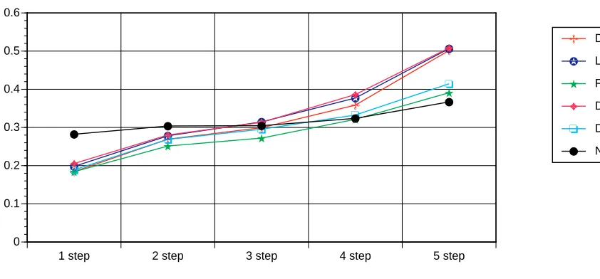
[image:16.612.96.517.149.345.2]

★ FGCV ✦ DFGCV ❏ DF2 ● NS Figure 1

Median MAPE for Price Errors over Forecast Horizon

4.2. Yield Errors

for price errors. The median MAPE increases steadily for all models except the NS model where the increase is less pronounced. We can see from Figure 1 that the NS median MAPE relatively improves at three steps ahead and becomes lower than all other models at ve steps ahead.

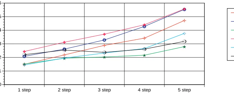
The average yield errors for all maturities for each method (averaged over the 26 quotation dates) are given in Table 3, with median yield errors over the quotation dates in Table 4. RMSE and MAE gures are given in basis points. Using median MAPE as a criterion, FGCV is best for two to ve steps ahead; similar results are obtained using RMSE and MAE. NS is best only at ve steps ahead using MAE while its second best at the same horizon using MAPE.

(17)

[image:17.612.101.501.163.332.2]

Figure 2

Median MAPE for Yield Errors over Forecast Horizon

✢

✪

★

★ ★ ★

★ ✦

✦

✧

✧ ✧

✧

❍

❍ _❍ ❍

❍

1 2 3 4 5 6

✢ DF1

✪ LDFGCV

★ FGCV

✦ DFGCV ✧ DF2 ❍ NS

4.3. Cost of the Second-Best Model

other modelsforecasts worsen with the forecast horizon. Overall, model FGCV is the best model both in terms of price and yield errors. NS appears to perform best when applied to longer-horizon forecasts.

(18)

✢

✢ ✢

✢

✪

✪ ✪

✪

★ ★ ★ ★

★

✦ ✦

✦

✖

✖ ✖

✖

✖ ❍

❍

❍ _❍

10 20 30 40 50 60

✢ DF1

✪ LDFGCV

★ FGCV ✦ DFGCV

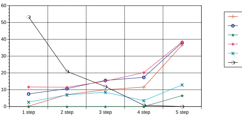
[image:18.612.97.512.149.360.2]

✖ DF2 ❍ NS Figure 3

Percentage Penalty over Best Method based on MAPE of Price Errors

4.4. Time Series Analysis of Results

error, the parsimonious model DF2 (splining the discount function with a xed number of knots: McCullochs method) has a very low penalty at one to three steps ahead (less than 20%) while the NS model has the lowest penalty at four and ve steps ahead.

(19)

✢

✪

✪ ✪

★

★ ★ ★ ★

✦

✩ ✩

✩

✩ ◆

◆

◆ ◆ _◆

20 40 60 80 100 120

✢ DF1

✪ LDFGCV

★ FGCV

✦ DFGCV

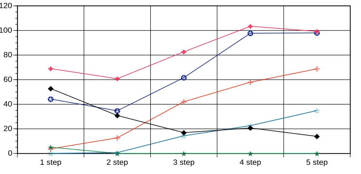
[image:19.612.100.471.162.341.2]

✩ DF2 ◆ NS Figure 4

Percentage Penalty over Best Method based on MAPE of Yield Errors

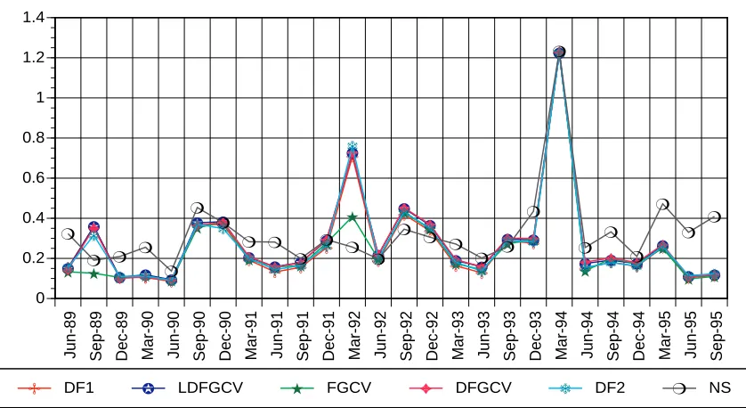
on 6 of 26 dates. The percentage of times that each model is best (in terms of MAPE) is given in Tables 7 and 8 for price and yield errors respectively. The most striking result is that the performance of the NS model closely trails that of the best model, FGCV, at the two- to four-step-ahead horizon for price errors. At ve steps ahead, model NS is best 42 per cent of the time as compared to only 31 per cent for the overall best model FGCV. Model NSs performance is even more impressive in terms of yield errors where it outperforms model FGCV at three to ve steps ahead, approaching a high of 54 per cent as compared to 31 per cent for model FGCV. Model DF2 does relatively well at short horizons in terms of yield errors, whereas the much less parsimonious model DF1 also does better in terms of price errors at short horizons (1-3 steps ahead). Given that the overall best model (model FGCV) fails to excel more than 50 per cent of the time suggests the need for further investigation of the performance of the models over time.

(20)

[image:20.612.104.523.166.395.2]

Figure 5

Time Series of Median MAPE of Price Errors from One-Step-Ahead Forecasts

✢ ✢ ✢ ✢ ✢ ✢ ✢ ✢ ✢ ✢ ✢ ✢ ✢ ✢ ✢ ✢ ✢ ✢ ✢ ✢ ✢ ✢ ✢ ✢ ✢ ✢ ✪ ✪ ✪ ✪ ✪ ✪ ✪ ✪ ✪ ✪ ✪ ✪ ✪ ✪ ✪ ✪ ✪ ✪ ✪ ✪ ✪ ✪ ✪ ✪ ✪ ✪ ★ ★ ★ ★ ★ ★ ★ ★ ★ ★ ★ ★ ★ ★ ★ ★ ★ ★ ★ ★ ★ ★ ★ ★ ★ ★ ✦ ✦ ✦ ✦ ✦ ✦ ✦ ✦ ✦ ✦ ✦ ✦ ✦ ✦ ✦ ✦ ✦ ✦ ✦ ✦ ✦ ✦ ✦ ✦ ✦ ✦ ❄ ❄ ❄ ❄ ❄ ❄ ❄ ❄ ❄ ❄ ❄ ❄ ❄ ❄ ❄ ❄ _❄ ❄ ❄ ❄ ❄ ❄ ❄ ❄ ❄ ❄ ❍ ❍ ❍ ❍ ❍ ❍ ❍ ❍ ❍ ❍ ❍ ❍ ❍ ❍ ❍ ❍ ❍ ❍ ❍ ❍ ❍ ❍ ❍ ❍ ❍ ❍

Jun-89 _Sep-89 _Dec-89 Mar-90 Jun-90 _Sep-90 Dec-90 Mar-91 Jun-91 Sep-91 Dec-91 Mar-92 Jun-92 Sep-92 Dec-92 Mar-93 Jun-93 Sep-93 Dec-93 Mar-94 Jun-94 Sep-94 Dec-94 Mar-95 Jun-95 Sep-95 0 0.2 0.4 0.6 0.8 1 1.2 1.4

✢ DF1 ✪ LDFGCV ★ FGCV ✦ DFGCV ❄ DF2 ❍ NS

(21)

✢ ✢ ✢ ✢ ✢ ✢ ✢ ✢ ✢ ✢ ✢ ✢ ✢ ✢ ✢ ✢ ✢ ✢ ✢ ✢ ✢ ✢ ✢ ✢ ✢ ✢ ✪ ✪ ✪ ✪ ✪ ✪ ✪ ✪ ✪ ✪ ✪ ✪ ✪ ✪ ✪ ✪ ✪ ✪ ✪ ✪ ✪ ✪ ✪ ✪ ✪ ✪ ★ ★ ★ ★ ★ ★ ★ ★ ★ ★ ★ ★ ★ ★ ★ ★ ★ ★ ★ ★ ★ _★ ★ ★ ★ ★ ✦ ✦ ✦ ✦ ✦ ✦ ✦ ✦ ✦ ✦ ✦ ✦ ✦ ✦ ✦ ✦ ✦ ✦ ✦ ✦ ✦ ✦ ✦ ✦ ✦ ✦ ✿ ✿ ✿ ✿ ✿ ✿ ✿ ✿ ✿ ✿ ✿ ✿ ✿ ✿ ✿ ✿ ✿ ✿ ✿ ✿ ✿ ✿ ✿ ✿ ✿ ✿ ❍ ❍ ❍ ❍ ❍ ❍ ❍ ❍ ❍ ❍ ❍ ❍ ❍ ❍ ❍ ❍ ❍ ❍ ❍ ❍ ❍ ❍ ❍ ❍ ❍ ❍

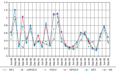
Jun-89 Sep-89 Dec-89 Mar-90 Jun-90 Sep-90 Dec-90 Mar-91 Jun-91 Sep-91 Dec-91 Mar-92 Jun-92 Sep-92 Dec-92 Mar-93 Jun-93 Sep-93 Dec-93 Mar-94 Jun-94 Sep-94 Dec-94 Mar-95 Jun-95 Sep-95 0 0.2 0.4 0.6 0.8 1 1.2 1.4

[image:21.612.107.549.271.547.2]

✢ DF1 ✪ LDFGCV ★ FGCV ✦ DFGCV ✿ DF2 ❍ NS Figure 6

(22)

✢ ✢

✢ ✢ ✢ ✢

✢

✢ ✢ ✢

✢ ✢

✢

✢ ✢ ✢ ✢

✢

✢ ✢ ✢ ✢ ✢ ❍

❍

❍ ❍ ❍ ❍ ❍ ❍ ❍ ❍

❍ ❍ ❍ ❍

❍

❍ ❍ ❍ ❍

❍ ❍

❍

❍ ❍ ❍ ❍

Jun-89 Sep-89 Dec-89 Mar-90 Jun-90 Sep-90 Dec-90 Mar-91 Jun-91 Sep-91 Dec-91 Mar-92 Jun-92 Sep-92 Dec-92 Mar-93 Jun-93 Sep-93 Dec-93 Mar-94 Jun-94 Sep-94 Dec-94 Mar-95 Jun-95 Sep-95 0

0.2 0.4 0.6 0.8 1 1.2 1.4 1.6

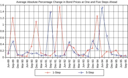
[image:22.612.98.523.139.401.2]

✢ 1-Step ❍ 5-Step Figure 7

Average Absolute Percentage Change in Bond Prices at One and Five Steps Ahead

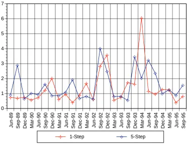
We compute the average absolute percentage change in bond prices and bond yields at each date of our sample in an attempt to measure shifts in the yield curve between the quote and the forecast dates. Figures 7 and 8 show plots of these series for bond prices and yields, respectively, at the one- and ve-steps-ahead forecast horizons.

(23)

✢ ✢ ✢ ✢ ✢ ✢

✢

✢ ✢

✢

✢ ✢

✢

✢ ✢ ✢ ✢

✢

✢ ✢ ✢

✢ ✢

✧ ✧

✧ ✧ ✧

✧

✧ ✧ ✧

✧

✧ ✧ ✧ ✧

✧

✧ ✧ ✧

✧

✧ ✧

✧

✧ ✧ _✧

✧

Jun-89 _Sep-89 _Dec-89 Mar-90 Jun-90 _Sep-90 _Dec-90 Mar-91 Jun-91 _Sep-91 _Dec-91 Mar-92 Jun-92 _Sep-92 _Dec-92 Mar-93 Jun-93 _Sep-93 _Dec-93 Mar-94 Jun-94 _Sep-94 _Dec-94 Mar-95 Jun-95 _Sep-95 0

1 2 3 4 5 6 7

[image:23.612.113.487.263.553.2]

✢ 1-Step ✧ 5-Step

Figure 8

(24)

13

4.5. Analysis of Whole Sample Results

When yield curve shifts are expressed in terms of yield changes, the NS model has the lowest correlation at one-step-ahead, while model FGCV has the highest correlation.

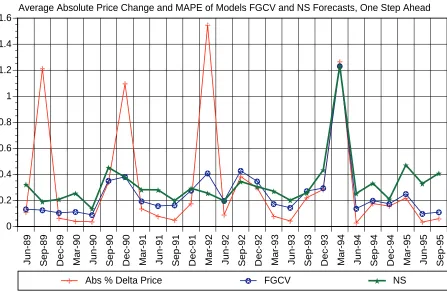
report simple correlation coefficients of the price and yield change and the price MAPE series over our 26 sample dates. The correlations between price MAPE and average price and yield changes are positive and quite high at one-step-ahead for all models; in general they are much lower at two- to ve-steps-one-step-ahead. In fact, they become negative at the four-step-ahead horizon, suggesting that models forecasting performance improves the larger the absolute change in the yield curve. Note that the overall best model, FGCV, and model NS, have the lowest correlations at one-step-ahead when we express movements in the yield curve in terms of price changes. This reects the results illustrated in Figures 5 and 6 and is also apparent in Figure 9, which plots the average price change series against the median price MAPE for models FCGV and NS. Figure 9 in-dicates that model FGCVs and NSs MAPEs do not increase commensurately with the price change on those dates with large price changes, such as Sep. 1989, Dec. 1990, March 1992, and March 1994.

Before we turn to evaluating the modelsforecast performance in various matu-rity ranges, let us summarize the results we have so far for the whole sample (all maturities). As previously stated, our comparison centers on the models ability to predict bond prices and yields up to ve days ahead, thus testing the models in an actual out-of-sample setting. Several main conclusions emerge from this analysis.

(25)

sam-✢ ✢ ✢ _✢ _✢ ✢ ✢ ✢ ✢ _✢ ✢ ✢ ✢ ✢ ✢ ✢ ✢ ✢ ✢ ✢ ✢ ✢ _✢ ✢ ✢ ✢ ✪ ✪ _✪ ✪ _✪ ✪ ✪ ✪ ✪ ✪ ✪ ✪ ✪ ✪ ✪ ✪ _✪ ✪ ✪ ✪ ✪ ✪ ✪ ✪ ✪ ✪ ★ ★ ★ ★ ★ ★ ★ ★ ★ ★ ★ ★ ★ ★ ★ _★ ★ ★ ★ ★ ★ ★ ★ ★ ★ ★

Jun-89 Sep-89 Dec-89 Mar-90 Jun-90 Sep-90 Dec-90 Mar-91 Jun-91 Sep-91 Dec-91 Mar-92 Jun-92 Sep-92 Dec-92 Mar-93 Jun-93 Sep-93 Dec-93 Mar-94 Jun-94 Sep-94 Dec-94 Mar-95 Jun-95 Sep-95 0 0.2 0.4 0.6 0.8 1 1.2 1.4 1.6

[image:25.612.101.548.252.545.2]

✢ Abs % Delta Price ✪ FGCV ★ NS

Figure 9

(26)

ple dates, the highly parameterized model DF1 (splining the discount function with a large number of knots) is always best in sample. In terms of yield errors, model FGCV (splining the forward rate curve with GCV) excels out-of-sample (from two to ve steps ahead) but only for one to three steps ahead for price errors. Interestingly, the NS model, estimated from STRIPS data, is best for the longest horizon price forecast (ve steps ahead) and second best at the ve-step horizon in terms of yield errors. At long horizons, the loss in forecast accuracy (as measured by percentage increase in MAPE) from using the wrong model is as high as 40% for price errors and 100% for yield errors. Overall, models DFGCV (splining the discount function with GCV) and LDFGCV (splining the log of the discount function with GCV) appear to be the least reliable at all forecasting horizons.

Second, comparing the models over time suggests that relying solely on mea-sures of average performance may overstate the case for the overall best model (FGCV). Particularly, model FGCV is best at most in 42% and 38% of the cases for price and yield errors respectively. In terms of price errors, models DF1 and NS closely track the overall best model for short and longer horizons respec-tively. In terms of yield errors, DF2 is best at least 26% of the time for short horizons while NS is best in up to 54% of the cases at the ve-step horizon.

(27)

4.6. Performance by Tenor Category

movements in the yield curve.

A common difficulty with any term structure estimation method is presented by the convexity of the price/yield relation, which causes price and yield er-rors of very different magnitudes to be generated along the yield curve. Many estimation techniques have attempted to account for this relation by duration weighting, minimizing the product of price and yield errors, and so on. Our goal in this study is not to add to this arsenal of methodology, but to evaluate the suitability of several techniques. It is likely that a technique which works quite well at short maturities may not exhibit the same performance at long maturities, and vice versa. To consider the relative suitability of the several techniques for securities of short, medium and long tenors, we summarize ex ante forecast performance for four tenor categories: 0-3 years, 3-7 years, 7-15 years, and greater than 15 years to maturity, where the category for a particular security is dened by its current remaining term.

More than half of the price quotations used in the analysis are associated with securities with no more than three years to maturity. Between 49% and 52% of the quotations fall in this range, with an additional 23% (22-26%) as-sociated with securities in the 3-7 year tenor range. On average, 15% (12-17%) of the quotations are associated with medium-term tenors (from 7 to 15 years to maturity) while the remaining 11% (10-14%) are associated with longer term securities. The heavy weight given to short-term (0-3 year) securities in our analysis suggests that forecasting reliability must be associated with reasonable performance at the short end of the yield curve.

(28)

penalty (in terms of median MAPE) incurred by choosing a method other than the best method for each forecast horizon and method. In the short-term tenor bracket, model FGCV is superior at all but the one-step-ahead horizon, while model NS is the least accurate method at each horizon. In the 37 year bracket, model NS performance steadily improves, surpassing model FGCV by small margins at four and ve steps ahead. Models DF1 and LDFGCV are also contenders in this bracket; in the 7-15 year bracket, model DF1 is marginally superior to FGCV at two steps ahead, with model NS superior at four and ve steps ahead. A somewhat similar pattern is realised for long-term securities, where model DF1 is superior at one and four steps ahead, model FGCV only at the two-step-ahead horizon, and model NS taking the remaining horizons. Thus, there are few clear lessons to be learned at medium to long tenors; model FGCVs performance never bears more than a ten per cent penalty over the best model, but it is not dominant in those three brackets. For short-term securities, the picture is clear, with model FGCV superior by a considerable margin. The three- to ve-step-ahead price error in that 03 year category is in the range of 10 to 12 cents per $100.00. Substantially greater errors are realised at longer horizons; ve-step-ahead price errors range from 43 cents (at 37 years) to 79 cents (at 15-30 years) per $100.00, reecting the convexity of the price-yield relation.

(29)

4.7. Performance for Treasury Bills

from the in-sample results, one would not consider this method a success, but the out-of-sample forecasting performance is much stronger. The penalty for unconditional use of model FGCV is somewhat higher for the 37 year and 15 30 year categories, with model FGCV underperforming model NS by up to 17 per cent and 16 per cent, respectively. The yield errors (measured by median MAPE) decline with tenor, amounting to 24 per cent for short-term securities, but only about one per cent for long-term securities. At a 7% yield, this would amount to about 30 basis points on a short-term security, and under 10 basis points for a long-term security.

All of the methods applied here make use of Treasury Bill quotations to anchor the short end of the estimated term structure. Some researchers (e.g. Bliss, 1997) have found that term structure estimation methods which use both bill quotations and coupon security quotations perform very poorly in predicting Treasury bill prices and/or yields. Since Treasury bill pricing is an essential element of many strategies in the interest rate derivatives markets, poor per-formance would be of considerable concern. Accordingly, we investigate the reliability of the six methods applied in this paper over the set of Treasury bill quotations in terms of ex ante forecast accuracy. There are between 30 and 33 Treasury bills in each quotation days dataset: roughly half of the quo-tations available in the 0-3 year tenor category considered above. Table 15 presents the median MAPE for Treasury bill price and yield prediction over the 26 quote dates, while Table 16 presents the percentage penalty (in terms of median MAPE) suffered by choosing a method other than the best method for each forecast horizon and method.

(30)

5. Conclusions

horizons of three, four and ve days ahead, while model DF2 (using a xed number of knots) is either rst- or second-best at all horizons, with similar MAPE statistics for all but the ve-day horizon. The Nelson-Siegel (NS) model is never better than third, with sizable penalties over the best model at all horizons. This same pattern of ndings holds for yield errors, in which model FGCV is again superior for three-step-ahead or longer forecasts (while exhibiting much weaker performance on the quote date). Model DF2 is also quite reliable, with percentage penalties of no more than 35% over model FGCV in terms of median MAPE.

In summary, then, it appears that model FGCV performs quite well in terms of ex ante forecasts of Treasury bill prices and yields. At the three-, four- or ve-day forecasting horizon, this model achieves percentage pricing errors of two to three cents per $100.00 and percentage yield errors of 1.5 to 3.0 per cent equivalent to less than 20 basis points at rates of 57%. Considering that the models generating these errors have not been t over bills alone, this would seem to be very respectable performance indeed. A serious effort to generate ex ante forecasts of Treasury bill prices and yields would presumably consider only bill quotations, but would have limited ability to improve upon the forecasting results summarized here.

(31)

models price and yield forecasting accuracy depends on the forecast horizon, an issue of likely interest to many practitioners. We evaluate ve splining method-ologies that differ in the choice of function which is splined and the degree to which the parameterization is determined by the data. The sixth method is the well-known Nelson-Siegel approach, in which the yield curve is derived from a second-order differential equation applied to Treasury coupon STRIPS data.

On average over the 26 sample dates, model FGCV (splining the forward rate curve with generalized cross-validation) produces the lowest out-of-sample price and yield forecast errors for most horizons. The model appears to perform particularly well for securities with 0-3 years to maturity in terms of price errors and for all securities up to 15 years to maturity in terms of yield errors. We nd that model FGCV is best in terms of price and yield forecasts for Treasury bills at the three-to ve step ahead horizons. This contradicts ndings reported by Bliss (1997) indicating that this splining methodology is not appropriate for modeling short-maturity securities prices or yields.

When we compare the models over time, we nd that the overall best model (FGCV) is best at most in 42% and 38% of the cases for price and yield errors respectively. Surprisingly, the highly parsimonious NS model excels at long forecast horizons: up to 42% of cases for price errors and 54% for yield errors. Of the splining methodologies, models LDFGCV (splining the log of the discount function with GCV) and DFGCV (splining the discount function with GCV) are always dominated, whereas model DF2 (splining the discount function with a xed number of knots: McCullochs method) is best in up to 38% of the short horizon forecasts of yield errors.

(32)

(33)

Table 1: Average Price Errors for All Maturities

0.247152

0.450985 0.502758 0.538717 0.578643 0.683226

0.118641

0.287469 0.338654 0.370442 0.406943

0.481311

0.104275

0.252339 0.297143 0.326710 0.360812 0.429919

bold

(a) Root Mean Squared Error

DF1 LDFGCV FGCV DFGCV DF2 NS Quote 0.280955 0.279429 0.276835 0.282603 0.415137 1-S 0.467394 0.489547 0.486379 0.483983 0.550584 2-S 0.530724 0.549203 0.546171 0.543202 0.589320 3-S 0.615749 0.632083 0.629263 0.598356 0.592420 4-S 0.644560 0.660581 0.657753 0.630593 0.623941 5-S 0.821705 0.834508 0.831851 0.784347 0.706681

(b) Mean Absolute Error

(c) Mean Absolute Percentage Error

(34)

Table 2: Median Price Errors for All Maturities

0.249058 0.328411 0.425066

0.499083 0.515831 0.586355

0.114763 0.204302

0.28549 0.325941 0.361164

0.391155

0.100066

0.184126 0.25142 0.272283 0.321386

0.366991 bold

(35)

Table 3: Average Yield Errors for All Maturities

11.0772

15.9735 18.0754

20.2626 26.6707 36.2815

5.16757

9.86506 11.5189 12.7975 14.6303 17.4074

1.00716

1.77939 2.12751

2.37139 2.60819 3.13233

bold

(36)

Table 4: Median Yield Errors for All Maturities

10.419

14.315 15.871 17.331 24.0774

28.8863

4.61009

8.1234 11.039 11.7972

14.0802

14.8385

0.855686

1.44465 1.94167

2.03273 2.16549 2.79604

bold

(37)

Table 5: Best and Runner-Up Models by Date and Horizon, MAPE of Price Errors

Date Quote 1-Step 2-Step 3-Step 4-Step 5-Step

Jun-89 DF1,DF2 FGCV,DFGCV FGCV,DFGCV FGCV,DFGCV FGCV,DF2 FGCV.NS

Sep-89 DF1,LDFGCV FGCV,NS NS,FGCV NS,FGCV NS,FGCV NS,FGCV

Dec-89 DF1,LDFGCV DFGCV,FGCV DF1,DFGCV DFGCV,DF1 DFGCV,LDFGCV DFGCV,DF2

Mar-90 DF1,DF2 DF1,DFGCV FGCV,DFGCV NS,FGCV NS,FGCV NS,FGCV

Jun-90 DF1,FGCV DF1,FGCV FGCV,DFGCV FGCV,DFGCV DFGCV,DF2 DF2,DFGCV

Sep-90 DF1,DF2 FGCV,DFGCV FGCV,DFGCV FGCV,DFGCV FGCV,DF2 FGCV,NS

Dec-90 DF1,FGCV DF2,DF1 DF1,DFGCV FGCV,NS FGCV,DF1 FGCV,DF1

Apr-91 DF1,DF2 DF1,FGCV FGCV,DF1 DF2,FGCV DF2,FGCV DF2,FGCV

Jun-91 DF1,DF2 DF1,DF2 DF1,DF2 DF1,FGCV DF1,DF2 DF2,DF1

Sep-91 DF1,DF2 DF1,FGCV DF1,FGCV FGCV,NS NS,FGCV NS,FGCV

Dec-91 DF1,DF2 DF1,DF2 DF2,DF1 DF1,DF2 NS,FGCV NS,FGCV

Mar-92 DF1,FGCV NS,FGCV NS,FGCV NS,FGCV NS,FGCV NS,FGCV

Jun-92 DF1,DF2 DF1,NS NS,FGCV NS,FGCV NS,FGCV NS,FGCV

Sep-92 DF1,DF2 NS,DF1 NS,FGCV NS,FGCV NS,FGCV FGCV,DF2

Dec-92 DF1,DF2 NS,DF1 NS,DF1 NS,FGCV DF1,DF2 NS,FGCV

Mar-93 DF1,FGCV DF1,FGCV DF1,DF2 DF1,FGCV FGCV,DF1 FGCV,DF1

Jun-93 DF1,DF2 DF1,DF2 NS,FGCV FGCV,DF2 FGCV,DF2 NS,FGCV

Sep-93 DF1,FGCV NS,FGCV NS,FGCV NS,FGCV NS,FGCV NS,FGCV

Dec-93 DF1,DF2 DF1,DF2 DF1,DF2 DF1,DF2 FGCV,DF1 NS,FGCV

Mar-94 DF1,DF2 LDFGCV,DF2 DF2,DF1 DF1,DF2 DF1,DF2 DF2,DF1

Jun-94 DF1,DF2 FGCV,DF1 FGCV,DF1 FGCV,NS FGCV,NS FGCV,NS

Sep-94 DF1,DF2 DF2,DF1 DF1,DF2 DF2,DF1 DF2,DF1 DF2,DF1

Dec-94 DF1,DF2 DF1,DF2 FGCV,DF1 DF1,DF2 FGCV,DF2 DF1,DF2

Mar-95 DF1,LDFGCV FGCV,DF1 FGCV,DF1 FGCV,DF1 FGCV,DF1 FGCV,DF2

Jun-95 DF1,DF2 FGCV,DF1 FGCV,DF2 FGCV,DF2 FGCV,NS FGCV,NS

(38)

Table 6: Best and Runner-Up Models by Date and Horizon, MAPE of Yield Errors

date Quote 1-Step 2-Step 3-Step 4-Step 5-Step

Jun-89 DF1,DF2 DFGCV,FGCV FGCV,NS FGCV,NS FGCV,NS FGCV,NS

Sep-89 DF1,DF2 FGCV,NS NS,FGCV NS,FGCV NS,FGCV NS,FGCV

Dec-89 DF1,DF2 DF2,FGCV NS,FGCV NS,FGCV NS,FGCV NS,FGCV

Mar-90 DF1,DF2 DFGCV,FGCV FGCV,DFGCV NS,FGCV NS,FGCV NS,FGCV

Jun-90 DF1,DF2 FGCV,DFGCV FGCV,NS FGCV,NS NS,DF2 NS,FGCV

Sep-90 DF1,DF2 FGCV,DFGCV FGCV,NS FGCV,NS FGCV,NS NS,FGCV

Dec-90 DF1,DF2 NS,DF1 NS,DF1 NS,FGCV NS,FGCV NS,FGCV

Apr-91 DF1,DF2 FGCV,DF2 FGCV,DF2 FGCV,DF2 NS,FGCV NS,FGCV

Jun-91 DF1,DF2 DF2,DF1 DF2,DF1 DF2,DF1 DF2,DF1 NS,FGCV

Sep-91 DF2,DF1 DF2,FGCV FGCV,NS NS,FGCV FGCV,DF2 NS,FGCV

Dec-91 DF1,DF2 DF1,NS DF2,DF1 NS,FGCV NS,FGCV NS,FGCV

Mar-92 DF1,FGCV NS,FGCV NS,FGCV NS, FGCV NS,FGCV NS,FGCV

Jun-92 DF1,FGCV FGCV,DF1 NS,FGCV NS,FGCV NS,FGCV NS,FGCV

Sep-92 DF1,DF2 NS,FGCV NS,FGCV NS,FGCV NS,FGCV FGCV,DF2

Dec-92 DF1,DF2 NS,DF1 NS,DF1 NS,DF1 NS,DF2 DF1,FGCV

Mar-93 DF1,FGCV DF1,FGCV DF2,FGCV FGCV,DF2 FGCV,NS FGCV,NS

Jun-93 DF1,DF2 DF1,DF2 NS,DF2 DF2,FGCV FGCV,DF2 NS,FGCV

Sep-93 DF1,FGCV FGCV,DF2 FGCV,DF2 FGCV,DF2 FGCV,NS FGCV,NS

Dec-93 DF1,DF2 DF2,DF1 DF2,DF1 DF2,FGCV DF2,FGCV NS,FGCV

Mar-94 DF1,DF2 FGCV,DF1 DF2,DF1 DF2,DF1 DF2,DF1 DF2,FGCV

Jun-94 DF1,DF2 DF1,DF2 DF2,DF1 DF2,DF1 DF2,FGCV FGCV,DF2

Sep-94 DF1,DF2 DF2,DF1 DF2,DF1 DF2,DF1 DF2,DF1 DF2,FGCV

Dec-94 DF1,DF2 DF2,DF1 DF2,DF1 DF2,DF1 DF2,FGCV DF2,FGCV

Mar-95 DF1,DF2 DF2,FGCV FGCV,DF2 FGCV,DF2 FGCV,DF2 FGCV,DF2

Jun-95 DF1,LDFGCV FGCV,DFGCV FGCV,DF2 FGCV,DF2 FGCV,DF2 FGCV,DF2

(39)

Table 7: Percentage of Cases in which each model is best, MAPE of Price Errors

Table 8: Percentage of Cases in which each model is best, MAPE of Yield Errors

model 1-Step 2-Step 3-Step 4-Step 5-Step DF1 42.31 26.92 23.08 11.54 3.85 LDFGCV 3.85 0.00 0.00 0.00 0.00 FGCV 26.92 38.46 38.46 42.31 30.77 DFGCV 3.85 0.00 3.85 7.69 3.85 DF2 7.69 7.69 7.69 7.69 19.23 NS 15.38 26.92 26.92 30.77 42.31

(40)

Table 9: Correlations between Average Price Change and MAPE of Price Errors

Table 10: Correlations between Average Yield Change and MAPE of Price Errors

model 1-Step 2-Step 3-Step 4-Step 5-Step DF1 0.80 0.31 0.38 -0.17 0.06 LDFGCV 0.80 0.31 0.37 -0.17 0.07 FGCV 0.62 0.37 0.18 -0.07 -0.06 DFGCV 0.79 0.30 0.36 -0.18 0.08 DF2 0.79 0.30 0.21 -0.14 0.13 NS 0.42 0.32 0.10 -0.09 -0.03

Note: The price change series contains average absolute percentage changes in bond price.

model 1-Step 2-Step 3-Step 4-Step 5-Step DF1 0.85 0.62 0.47 -0.25 0.13 LDFGCV 0.86 0.64 0.48 -0.24 0.12 FGCV 0.92 0.75 0.56 -0.14 0.10 DFGCV 0.86 0.64 0.49 -0.24 0.13 DF2 0.85 0.61 0.52 -0.18 0.09 NS 0.80 0.58 0.38 -0.16 0.16

(41)

Table 11: Median MAPE of Price Errors by Tenor Category

0.041355

0.071831 0.099629

0.097156 0.125417 0.12643

0.0978682

0.218118 0.267204

0.328485

0.384470 0.431740

0.272192

0.423399 0.519443

0.580446

0.605199 0.712300

0.0541203 0.384072

0.593907

0.608901 0.633187

0.789631 bold

(a) Securities with 03 years to maturity

model DF1 LDFGCV FGCV DFGCV DF2 NS Full Quote 0.057647 0.056517 0.075278 0.045449 0.111705 0.100066 1-S 0.072474 0.094600 0.075782 0.094129 0.120954 0.184126 2-S 0.100925 0.115865 0.122959 0.102338 0.121619 0.251420 3-S 0.125254 0.145133 0.155753 0.116524 0.139872 0.272283 4-S 0.142055 0.160857 0.169119 0.136017 0.143571 0.321386 5-S 0.171021 0.189539 0.195266 0.158979 0.164866 0.366991

(b) Securities with 3-7 years to maturity

(c) Securities with 7-15 years to maturity

(d) Securities with 15-30 years to maturity

model DF1 LDFGCV FGCV DFGCV DF2 NS Full Quote 0.154805 0.143715 0.120204 0.149313 0.406867 0.100066 1-S 0.434007 0.3874 0.411932 0.422089 0.567215 0.184126 2-S 0.613553 0.616728 0.617579 0.60819 0.595221 0.251420 3-S 0.662924 0.678163 0.617893 0.671576 0.654702 0.272283 4-S 0.668914 0.693802 0.65907 0.665908 0.689437 0.321386 5-S 1.01554 1.02524 0.908154 1.0192 1.01229 0.366991 Note: minimum value over models for each tenor category presented in .

(42)

Table 12: Median MAPE of Yield Errors by Tenor Category

1.32526

1.95069 2.50592 2.80508

3.42076 3.88385

0.395073

0.903704 1.0878 1.2933

1.69910 1.63899

0.668106

0.905532 1.15224 1.25853 1.23922 1.44738

0.0747147 0.501944

0.769142

0.754363 0.868876

1.020520 bold

(b) Securities with 37 years to maturity

model DF1 LDFGCV FGCV DFGCV DF2 NS Full Quote 0.205923 0.184648 0.155663 0.198777 0.523428 0.855686 1-S 0.566058 0.511504 0.538426 0.559037 0.718061 1.44465 2-S 0.77826 0.780202 0.782415 0.783337 0.771668 1.94167 3-S 0.85119 0.875308 0.817194 0.856558 0.837093 2.03273 4-S 0.917675 0.923477 0.903982 0.919852 0.932578 2.16549 5-S 1.30013 1.31742 1.18038 1.30755 1.3068 2.79604 Note: minimum value over models for each tenor category presented in .

(43)

Table 13: Percentage Penalty of Price Errors by Tenor Category

model DF1 LDFGCV FGCV DFGCV DF2 NS Quote 0 39.3972 36.6643 82.0286 9.90057 170.113 1-S 0.895317 31.6986 5.50057 31.0428 0 68.386 2-S 1.30047 16.2969 0 23.4173 2.71908 22.071 3-S 28.92 49.3804 0 60.3112 19.9348 43.966 4-S 13.266 28.2575 0 34.8453 8.45185 14.475 5-S 35.2694 49.9162 0 54.4467 25.7454 30.410

model DF1 LDFGCV FGCV DFGCV DF2 NS Quote 0 1.99048 6.18355 5.99965 11.5771 175.821 1-S 7.8104 11.5958 0 8.6435 13.6838 30.9307 2-S 0 1.2156 1.97239 0.658413 4.32709 11.9422 3-S 13.4753 16.456 0 15.4171 18.7451 1.0227 4-S 16.6915 19.7157 4.6742 19.8937 19.3723 0 5-S 11.1456 7.0289 4.3501 7.4656 7.8434 0

model DF1 LDFGCV FGCV DFGCV DF2 NS Quote 0 11.195 11.6743 9.02855 21.6732 56.0174 1-S 1.37524 3.33812 0 3.36513 2.59014 18.4134 2-S 0 2.95234 0.49647 2.70207 2.83599 11.9198 3-S 8.20537 9.87485 0 10.563 0.752176 8.8804 4-S 4.0486 6.3489 0.6976 5.8074 2.4295 0 5-S 22.2408 22.4645 4.3698 21.9758 11.7949 0

(44)

Table 14: Percentage Penalty of Yield Errors by Tenor Category

model DF1 LDFGCV FGCV DFGCV DF2 NS Quote 0 74.359 39.497 127.326 6.80338 121.826 1-S 8.74013 70.8237 12.2756 115.279 0 68.1549 2-S 29.4497 55.5827 2.29091 92.9119 0 39.0216 3-S 51.4088 91.0952 0 110.235 12.8384 17.0350 4-S 51.9255 100.933 0 124.876 9.49206 5.7036 5-S 87.8921 135.158 0 143.321 35.4383 5.9479

model DF1 LDFGCV FGCV DFGCV DF2 NS Quote 0 1.81411 4.21152 7.01664 5.64088 167.658 1-S 9.40314 15.4365 0 13.098 13.5257 24.7963 2-S 0.557036 4.35391 0 3.27253 6.87253 6.7627 3-S 22.9409 22.8862 0 21.717 25.1636 6.9973 4-S 16.8249 18.3662 0.8764 17.8855 18.1136 0 5-S 55.9464 50.4067 16.6375 50.8926 45.1514 0

model DF1 LDFGCV FGCV DFGCV DF2 NS Quote 0 5.4816 7.04332 5.83323 8.37647 40.2823 1-S 9.57304 11.7522 0 12.0444 10.1491 24.4170 2-S 12.4069 13.4718 0 13.0147 13.592 15.5446 3-S 13.7 13.7493 0 13.4013 11.3509 22.9136 4-S 12.1252 13.4039 0 13.4051 8.74673 7.4138 5-S 40.4684 42.0223 0 42.0712 25.764 1.6597

(45)

Table 15: Median MAPE for Treasury Bills

0.00880527

0.0145105 0.0196475 0.0228137

0.0250907 0.0244604

0.796772

1.18681 1.58425 1.52563

2.13098 2.92778

bold

(a) Price Errors

model DF1 LDFGCV FGCV DFGCV DF2 NS

Quote 0.020914 0.0177765 0.0276213 0.00976778 0.052031 1-S 0.015862 0.0313875 0.0203268 0.0353665 0.048836 2-S 0.0250686 0.0428039 0.0210726 0.0432806 0.047613 3-S 0.0319612 0.0566628 0.0552664 0.026548 0.049468 4-S 0.0432801 0.066793 0.0661124 0.0308675 0.058193 5-S 0.0638737 0.0809441 0.0856178 0.0491018 0.051764

(b) Yield Errors

model DF1 LDFGCV FGCV DFGCV DF2 NS Quote 1.60218 1.49004 2.14318 0.961537 4.80937 1-S 1.44603 2.5043 1.28598 3.25211 3.93438 2-S 2.28349 3.40034 1.63677 3.81861 4.59787 3-S 3.30232 4.18825 5.13248 2.07375 4.26124 4-S 4.33967 5.31338 6.08526 2.75941 4.91517 5-S 5.964 7.15206 7.81706 3.69184 4.74682

(46)

Table 16: Percentage Penalty for Treasury Bill Prediction

(a) Price Errors

model DF1 LDFGCV FGCV DFGCV DF2 NS Quote 0 137.517 101.884 213.691 10.9311 490.904 1-S 9.31417 116.309 40.0836 143.731 0 236.557 2-S 27.5919 117.86 7.2537 120.286 0 142.337 3-S 40.097 148.372 0 142.251 16.3687 116.837 4-S 72.4947 166.207 0 163.494 23.0239 131.931 5-S 161.131 230.919 0 250.026 100.74 111.623

(b) Yield Errors

(47)

References

Computer Science in Economics and

Man-agement

Ad-vances in Futures and Options Research

A practical guide to splines

Journal of Banking and Finance

Journal of Finance

Journal of Political Economy

Econometrica

Econo-metrica

Numerische Mathematik

[1] Baum, C.F. and C. F. Thies, 1992, On the construction of monthly term structures of U.S. interest rates,

, 5, 221-46.

[2] Bliss, Robert R., 1997, Testing term structure estimation methods, , 9, 197-231.

[3] de Boor, C., 1978, , Applied Mathematical Sci-ences, Vol. 27. Springer, New York.

[4] Brennan, M.J., and E.S. Schwartz, 1979, A continuous time approach to the pricing of bonds, 3, 133-55.

[5] Carleton, W. and I. Cooper, 1976, Estimation and uses of the term structure of interest rates, 31, 1067-83.

[6] Cecchetti, S., 1988, The case of negative nominal interest rates: new esti-mates of the term structure of interest rates during the Great Depression,

96(6), 1111-41.

[7] Cox, J., J. Ingersoll, and S. Ross, 1985a, An intertemporal general equilib-rium model of asset prices, 53, 363-84.

[8] , 1985b, A theory of the term structure of interest rates, 53, 385-467.

(48)

Mathematica

Journal of Finance,

Computational

Eco-nomics and Finance: Modeling and Analysis with

Jour-nal of Business

Journal of Finance

Journal of Business

Journal of Financial and Quantitative Analysis

Journal of Financial Economics

[10] Duffie, Darrell, 1996, Special Repo Rates, 51:2, 493-526.

[11] Fisher, M.E., Nychka, D., and D. Zervos, 1995, Fitting the term structure of interest rates with cubic splines, FEDS discussion paper 95-1, Federal Reserve Board of Governors.

[12] Fisher, M.E. and D. Zervos, 1996, Yield Curve, in

, H. Var-ian, ed. Springer-Verlag, New York.

[13] Gilles, Christian, 1997, private communication with the second author. [14] McCulloch, J.H., 1971, Measuring the term structure of interest rates,

, 44, 19-31.

[15] , 1975, The tax-adjusted yield curve, , 30, 811-30.

[16] Nelson, C.R. and A.F. Siegel, 1987, Parsimonious Modeling of Yield Curves, , 60, 473-89.

[17] Shea, G.S., 1984, Pitfalls in smoothing interest rate term structure data, , 19 (3), 253-69.