Evolution of a compound droplet attached to a core-shell nozzle under the action of a strong electric field

Evolution of a compound droplet attached to a core-shell nozzle

under the action of a strong electric field

S. N. Reznik, A. L. Yarin,a兲E. Zussman, and L. Bercovici

Faculty of Mechanical Engineering, Technion-Israel Institute of Technology, Haifa 32000, Israel

共Received 2 December 2005; accepted 1 May 2006; published online 20 June 2006兲

The shape evolution of small compound droplets at the exit of a core-shell system in the presence of a sufficiently strong electric field is studied both experimentally and theoretically. It is shown that the jetting effect at the tip of the shell nozzle does not necessarily cause entrainment of the core fluid, in which case the co-electrospinning process fails to produce core-shell nanofibers. The remedy lies in extending the core nozzle outside its shell counterpart by about half the radius of the latter. The results also show that the free charges migrate very rapidly from both fluids and their interface to the free surface of the shell. This reflects the fact that most of the prejetting evolution of the droplet can be effectively described in terms of the perfect conductor model, even though the fluids can be characterized as leaky dielectrics. The stress level at the core-shell interface is of the order of 5⫻103_{g /共cm s}2_{兲, the relevant value in assessing the viability of viruses, bacteria, DNA}

molecules, drugs, enzymes, chromophores, and proteins to be encapsulated in nanofibers via co-electrospinning. ©2006 American Institute of Physics.关DOI:10.1063/1.2206747兴

I. INTRODUCTION

Co-electrospinning was proposed for manufacturing core-shell meso/nanofibers made of two different polymer materials.1–5 Polymer solutions 共in immiscible or miscible solvents兲 are supplied from a spinneret consisting of two coaxial capillaries. At the spinneret exit a core-shell droplet emerges. In the presence of a sufficiently strong electric field, such a droplet cannot sustain any steady-state configu-ration, and jetting sets in at its tip. In many cases the jet entrains only the shell solution, while that of the core is unaffected, so that even though the droplet has a core-shell structure, co-electrospinning does not occur. By contrast in other cases the core-shell structure is preserved in the out-flowing jet and co-electrospinning proceeds properly. The jet exhibits the electrically induced bending instability initially discovered in electrospinning of single-fluid jets,6–9 which results in strong stretching of the bending sections of the jet. The solvent eventually evaporates, the jet dries and solidi-fies, and as-spun fibers共with the core-shell structure and di-ameters typically in the submicron range兲are deposited on a counterelectrode共ground兲.

In Refs. 2 and 10 ceramic sol-gel precursors were added to the shell solutions to yield ceramic nanofibers, with the core material共a heavy mineral oil兲 later extracted with oc-tane. In Ref. 11 core-shell polymethyl methacrylate/ polyacrylonitrile共PMMA/PAN兲nanofibers were post-treated at high temperature in an oven, with the PMMA fully de-graded共the gaseous products driven off兲 and the PAN car-bonized; by this means, turbostratic carbon nanofibers were manufactured.

The experiments on co-electrospinning1,11show that

co-electrospun jets exhibit standard bending instability, prob-ably affected to some extent by the two-fluid jet structure. However, the analysis of the as-spun nanofibers shows that in several cases they do not possess a core-shell structure. For example, Fig. 1 shows nanofibers made via co-electrospinning of two polymer solutions: polymethyl meth-acrylate共PMMA兲in the core and polyacrylonitrile共PAN兲in the shell. The as-spun core-shell nanofibers were carbonized at elevated temperatures following Ref. 11. As a result, PMMA in the core was fully degraded and left the core as a volatile constituent, whereas PAN in the shell has been trans-formed into turbostratic carbon. The resulting carbon nanofi-bers in Fig. 1 are hollow, whereas the numerous intact carbon nanofibers also seen in the figure manifest the fact that PMMA solution has not been entrained in the as-spun jet, and the core-shell structure did not emerge. Therefore, for polymeric fluids typical to co-electrospinning, the question whether and when a core-shell jet can be formed is obviously cardinal. On the other hand, linear stability analysis which indeed elucidates the bending instability of the core-shell jets

共albeit under a very restrictive assumption of the inviscid flow12兲does not address this practically important question. The main aim of the present work is to elucidate the condi-tions under which the jet will consist of core fluid共supplied by the central pipe兲surrounded by an outer shell originating in the fluid supplied by the annular pipe. That is the main theoretical issue related to co-electrospinning in light of the experimental work in Ref. 11.

In certain cases the polymer solutions used in co-electrospinning can serve as carriers for viruses, bacteria, and drugs such as fungicides.13,14Such nanofibers can also incor-porate DNA molecules in their core. Since at a certain stress level in the flow the viruses, bacteria, DNA molecules and drugs may be damaged and lose their viability, an electrohy-drodynamic theory of jet formation in co-electrospinning

a兲_{Author to whom correspondence should be addressed. Present address:}

Department of Mechanical and Industrial Engineering, University of Illi-nois at Chicago, 842 West Taylor Street, Chicago, IlliIlli-nois 60607-7022. Electronic mail: [email protected]

should also take account of the stress level in the fluids—an additional aim of the present work.

Transient evolution of single-fluid drops in electric fields was the subject of Refs. 15–19. Of these, Refs. 16 and 17 effectively dealt with inviscid fluids developing potential flows—the case typically corresponding to electrospraying, whereas Ref. 19 considered the flow in the drop as a creeping flow, characteristic of electrospinning of polymer solutions. The present work generalizes this approach of Ref. 19 to the two-fluid case, appropriate for co-electrospinning.

The problem is posed in Sec. II. The dimensionless pa-rameters are listed in Sec. III and the numerical method is described in Sec. IV. The experimental setup is described in Sec. V. The results are presented and discussed in Sec. VI. Conclusions are drawn in Sec. VII.

II. PROBLEM FORMULATION

A core-shell nozzle consists of a central cylindrical pipe and a concentric annular pipe surrounding it 共cf. Fig. 2兲, through which two different fluids are supplied separately. As a result, two-component共core-shell兲droplets are formed at the nozzle exit. When the process takes place without an applied electric field, the outer surface of the droplet and the interface between its components acquire near-spherical equilibrium shapes due to the action of the surface and inter-facial tension, respectively. If after establishment of the equi-librium shape an electric field is applied to the compound nozzle and droplet共attached to an electrode immersed in it, with a counterelectrode, say a metal plate, located at some distance from the droplet tip兲, the latter undergoes stretching under the action of Maxwell stresses of electric origin. In these circumstances it can be restabilized in a new elongated shape by the surface and interfacial tension, or become fully transient until a jet issues from its tip. The stretching by the electric stresses proceeds with or without permanent supply of the two fluids through the core-shell nozzle.

Both the core and the shell fluids are considered as leaky dielectrics, whose electric relative permittivities and conduc-tivities are denoted as ␧in, ␧out, and ␴in, ␴out, respectively.

The compound droplet is in turn immersed in a leaky dielec-tric medium with relative permittivity␧sur and conductivity

␴sur 共in vacuum ␧sur= 1 and ␴sur= 0兲. The viscosities of the

fluids and the surrounding medium are denoted as␮in,␮out,

and␮sur, respectively. At t= 0 the initial shapes of the

inter-faces in Fig. 2 are given by spherical segments. It is assumed that the electric field is imposed at the initial time moment t= 0 and that at a distance r from the droplet, much larger

than the radius of the shell nozzler_out 共of the order of the initial radius of the shell fluid兲the field is uniform,E=E_⬁.

Our aim is to determine the droplet evolution in time in the presence of an the electric field. The problem is described by the following set of mechanical and electric equations and boundary conditions. The fluid motion is inertialess and gov-erned by the Stokes equations, which have the following form:

ⵜ·ui= 0, 共1兲

ⵜpi=␮i⌬ui, 共2兲

where p is pressure, u is the velocity vector, and the sub-script i= in, out, and sur refers to the inner, outer, and sur-rounding fluid, respectively. The problem is axisymmetric, so thatu has only two components, the radial urand the axial uz. The dynamic boundary conditions at the interfaces are given by

fi−fi+1=␥i,i+1␬n+fi+1

E −fi

E

, 共3兲

at⌫i,i+1withi= in or out, andi+ 1 = out or sur, respectively;f

and fE _{denote the total and the electric tractions per unit} surface area of the boundary,nis the unit outer normal at the boundary⌫i,i+1,␥i,i+1is the surface interfacial tension, and␬

is the curvature of the surface⌫i,i+1.

The electric tractions are related to the Maxwell stresses

␴␣␤E

f_␣E=␴_␣␤E n_␤, ␴_␣␤E = ␧i

4␲

冉

E␣E␤− 1 2E

2_␦

␣␤

冊

, 共4兲

where␴_␣␤ are the components of the electric stress tensor; the field strength componentsE_␣,E_␤and its magnitudeEare calculated via the corresponding electric potentials␾i, satis-fying the Laplace equation

ⵜ2_␾

i= 0, 共5兲

withEi= −ⵜ␾i.

The electric boundary conditions describe the jump in the normal component of the electric field and electric induc-tion at the boundaries

共Ei+1·n兲−共Ei·n兲= 4␲␳, x苸⌫i,i+1, 共6兲

␧i+1共Ei+1·n兲−␧i共Ei·n兲= 4␲q, x苸⌫i,i+1 共7兲

[image:2.612.68.282.51.123.2]

and the continuity of the tangential component of the electric field

FIG. 2. Core-shell droplet at the exit of a core-shell nozzle. All solid walls are assumed to be perfect conductors.

[image:2.612.375.497.51.143.2]

共Ei+1·␶兲=共Ei·␶兲, x苸⌫i,i+1, 共8兲

where␶is the unit tangent to the surface⌫i,i+1,q共x,t兲is the

free charge density at this surface,␳ is the overall共free and due to polarization兲 surface charge density. On the metal plate surface共⌫3 in Fig. 2兲the potential ␾sur=␾plate is

con-stant. We assume that this condition holds also on⌫₁and⌫₂. Then

␾= 0, x苸⌫1, ⌫2, or⌫3. 共9兲

The balance of the free charge at the surfaces is given by

dq

dt +d·q=␴i共Ei·n兲−␴i+1共Ei+1·n兲, x苸⌫i,i+1, 共10兲 whered=␶·⳵u/⳵s+ur/ris the local coefficient of the surface stretching for the axisymmetric case considered in the present work, andsis the arc length over the surface genera-trices,r=r共s,t兲. The initial condition to共10兲is

q共0,s兲=q0共s兲, 共11兲

whereq0_{共s兲 is the initial distribution of the charge density}

over the free surface or the interface. We shall assume in the following thatq0_{= 0, i.e., that the droplet was not charged or}

polarized att= 0共the free surface and the interface are also charge-free att= 0兲.

The kinematic boundary conditions at the surfaces are given by

dx

dt =u共x兲, 共12兲

wherex is the position vector at the free surface or at the interface. The initial position vectors correspond to points on the spherical segments共the boundary兲att= 0

x共0兲=x0. 共13兲

The contact lines at the walls are assumed to be “anchored,” so that at all the solid boundaries in contact with the fluids

u= 0. 共14兲

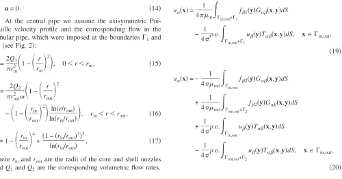
At the central pipe we assume the axisymmetric Poi-seuille velocity profile and the corresponding flow in the annular pipe, which were imposed at the boundaries⌫1and

⌫2共see Fig. 2兲:

uz= 2Q₁

␲r_in2

冉

1 −

冉

r r_in

冊

2

冊

, 0⬍r⬍r_in, 共15兲

uz= 2Q2

␲r_out2 ␻

冉

1 −

冉

r rout

冊

2

−

冉

1 −

冉

rin r_out

冊

2

冊

ln共r/r_out兲

ln共r_in/r_out兲

冊

, rin⬍r⬍rout, 共16兲

␻= 1 −

冉

rin r_out

冊

4

+共1 −共rin/rout兲

2_兲2

ln共r_in/r_out兲 , 共17兲

whererin androut are the radii of the core and shell nozzles

andQ1 andQ2 are the corresponding volumetric flow rates.

III. DIMENSIONLESS PARAMETERS

Introduce the following dimensionless variables:

x ¯ = x

rout

, t¯= t t0

, u¯ = u u0

, f¯i= rout

␮iu0

fi,

f ¯ i E

=fi E

/E_⬁2, ␬¯=␬r_out, 共18兲

E¯ =E/E_⬁, ¯q=q/E_⬁, ¯␳=␳/E_⬁, ␴¯i=t0␴i,

whereu0=␥out,sur/共␮out−␮sur兲,t0=rout/u0.

The main dimensionless parameters governing the evolution of the droplet are the electric Bond number BoE=routE_⬁2/␥out,sur, the ratio of the interfacial and surface

tensions␥in,out/␥out,sur, and the ratios of the viscosities.

IV. NUMERICAL METHOD

The governing Eqs. 共1兲, 共2兲, and 共5兲, rendered dimen-sionless and subject to the boundary conditions共3兲,共14兲, and

共6兲–共8兲are solved with the aid of equivalent boundary inte-gral formulations in which a set of corresponding inteinte-gral equations is solved.20,21As a result the values of u共x兲 and E共x兲 at the interfaces at each time moment are known and the droplet evolution can be determined by time stepping

共using the Kutta-Merson method兲 for Eqs. 共10兲 and 共12兲, with the initial conditions共11兲and共13兲.

[image:3.612.61.561.508.770.2]

Consider in detail the integral equation formulation for the case of a core-shell droplet at the nozzle exit shown in Fig. 2. For a pointx of the Lyapunov curve⌫in,out, the

fol-lowing dimensional integral equations hold:

u_␣共x兲= 1 4␲␮_in

冕

_⌫

in,out+⌫1

f_␤1共y兲G_␣␤共x,y兲dS

− 1 4␲p.v.

冕

_⌫

in,out+⌫1

u_␤共y兲T_␣␤共x,y兲dS, x苸⌫in,out,

共19兲

u_␣共x兲= − 1

4␲␮out

冕

⌫in,out

f_␤2共y兲G␣␤共x,y兲dS

+ 1

4␲␮out

冕

⌫out,sur+⌫2

f_␤2共y兲G␣␤共x,y兲dS

+ 1 4␲p.v.

冕

_⌫

in,out

u_␤共y兲T_␣␤共x,y兲dS

− 1 4␲p.v.

冕

_⌫

out,sur+⌫2

u_␤共y兲T_␣␤共x,y兲dS, x苸⌫in,out,

0 = − 1

4␲␮sur

冕

⌫out,sur

f_␤3共y兲G␣␤共x,y兲dS

+ 1

4␲␮_sur

冕

_⌫

3

f_␤3共y兲G_␣␤共x,y兲dS

+ 1

4␲p.v.

冕

_⌫out,suru␤共y兲T␣␤共x,y兲dS − 1

4␲p.v.

冕

_⌫

3

u_␤共y兲T_␣␤共x,y兲dS, x苸⌫_in,out, 共21兲 where

G_␣␤= ␦␣␤ rxy +

xˆ_␣xˆ_␤ rxy3

, T_␣␤= − 6xˆ␣xˆ␤xˆknk共y兲 rxy5

,

共22兲 rxy=兩x−y兩, xˆ_␣=x_␣−y_␣,

nis the outward unit normal vector to the boundaries, includ-ing⌫1,⌫2, and⌫3. Multiplying Eqs.共19兲–共21兲by␮in,␮out,

and␮_sur, respectively, adding them and dividing the sum by

␮in+␮out, we obtain the boundary integral equation 共BIE兲

containing the traction differences at the boundaries ⌫in,out

and⌫out,sur, just as in the boundary condition共3兲:

u_␣共x兲= 1

4␲共␮_in+␮_out兲

冕

_⌫

in,out

共f_␤1共y兲−f_␤2共y兲兲G_␣␤共x,y兲dS+ 1

4␲共␮_in+␮_out兲

冕

_⌫

out,sur

共f_␤2共y兲−f_␤3共y兲兲G_␣␤共x,y兲dS

+ 1

4␲共␮in+␮out兲

兺

i=1 3

冕

⌫i

f_␤i共y兲G␣␤共x,y兲dS− 1 4␲

␮in−␮out

共␮in+␮out兲

p.v.

冕

⌫in,out

u_␤共y兲T_␣␤共x,y兲dS

− 1 4␲

␮out−␮sur

共␮in+␮out兲

p.v.

冕

⌫out,sur

u_␤共y兲T_␣␤共x,y兲dS− 1

4␲共␮in+␮out兲

兺

i=1 3

␮i·p.v.

冕

⌫i

u_␤共y兲T_␣␤共x,y兲dS, x苸⌫_in,out. 共23兲 If pointx belongs to the boundary⌫1, the left-hand side in共20兲vanishes共the point lying outside the second fluid兲. The

BIE then acquires the form of共23兲with␮in+␮outreplaced by␮in. If the point belongs to the boundary⌫out,sur, subtraction of

the equations similarly to共19兲–共21兲yields the following BIE:

u_␣共x兲= 1

4␲共␮_out+␮_sur兲

冕

_⌫

in,out

共f_␤1共y兲−f␤2共y兲兲G␣␤共x,y兲dS+

1

4␲共␮_out+␮_sur兲

冕

_⌫

out,sur

共f_␤2共y兲−f␤3共y兲兲G␣␤共x,y兲dS

+ 1

4␲共␮out+␮sur兲

兺

i=1 3

冕

⌫i

f_␤i共y兲G␣␤共x,y兲dS− 1 4␲

␮in−␮out

共␮out+␮sur兲

p.v.

冕

⌫in,out

u_␤共y兲T_␣␤共x,y兲dS

− 1 4␲

␮out−␮sur

共␮out+␮sur兲

p.v.

冕

⌫out,sur

u_␤共y兲T_␣␤共x,y兲dS− 1

4␲共␮_out+␮_sur兲

兺

i=1 3

␮i·p.v.

冕

⌫i

u_␤共y兲T_␣␤共x,y兲dS, x苸⌫_out,sur.

共24兲 If the point belongs to the boundary⌫2共or⌫3兲, the BIE acquires the form of共24兲with␮out+␮surreplaced by␮out共or␮sur兲.

Using the boundary condition共3兲and the dimensionless variables共18兲, one can present all the above BIE’s in the form

u_␣共x兲=

兺

j=1 2

1 4␲

␮j−␮j+1

Mi

冋

冕

_⌫ j,j+1

t_␤共y兲G_␣␤共x,y兲dS−p.v.

冕

⌫j,j+1

u_␤共y兲T_␣␤共x,y兲dS

册

+

兺

j=1 3

1 4␲

␮j Mi

冋

冕

_⌫j

f_␤j共y兲G␣␤共x,y兲dS−p.v.

冕

⌫j

u_␤共y兲T_␣␤共x,y兲dS

册

, 共25兲

where

Mi=

再

␮i+␮i+1, ifx苸⌫i,i+1

␮i, ifx苸⌫i,

冎

共26兲

t共y兲=Ri,i+1关˜␥i,i+1␬n+ BoE共fi+1

E −fi

E_兲兴

, y苸⌫i,i+1,

Ri,i+1=

␮out−␮sur

␮i−␮i+1

, ␥˜i,i+1=

␥i,i+1

␥out,sur

, i=兵in,out其, 共27兲

i+ 1 =兵out,sur其,

considered in the present work, the tractionsf3= 0 and the

integrals over⌫3 vanish.

The BIE共25兲contains the electric stressesfi E

induced by the electric field E at the boundaries ⌫in,out and ⌫out,sur. To

find them, we resort to the boundary integral formulation used in Ref. 15 for the case of a dielectric droplet in a sur-rounding dielectric fluid. Here we deal with core-shell drop-lets consisting of two leaky dielectrics. We also use the mirror-image method to convert the core and shell free sur-faces into closed sursur-faces similar to the case of an isolated core-shell droplet. This is possible, because the plane metal electrode is assumed to be a perfect equipotential conductor. If a core-shell leaky dielectric droplet 共with closed free and interface surfaces plus their mirror images兲is located in an external electric fieldE_⬁, the charges can accumulate only at the boundaries ⌫in,out and⌫out,sur between the fluids with

different dielectric permittivities, and the fluid bulk is prac-tically neutral.22Then, according to Coulomb’s law the elec-tric field at an arbitrary pointx

⬘

共off the surfaces兲is given by

E=

兺

j=1 2

冕

⌫˜ j,j+1

␳共y兲Kˆ共x

⬘

,y兲dS

+E_⬁, x

⬘

苸⌫in,out, ⌫out,sur, 共28兲

where

Kˆ共x

⬘

,y兲=x

⬘

−y

r_x3_⬘y . 共29兲

␳ is the surface distribution of the overall charges共free and those due to polarization兲at the surfaces⌫˜j,j+1which include

⌫j,j+1and their mirror images.

Consider a pointx at the surface ⌫_in,out or ⌫_out,sur 共they are assumed to be of the Lyapunov type except for the con-tact lines connecting them and their mirror images atz= 0兲. Multiplying 共28兲 by n共x兲 and taking x

⬘

tending to x from both sides of the surface, we obtain23

共Ei·n兲=

兺

j=1 2

冕

⌫˜ j,j+1

␳共y兲K共x,y兲dS− 2␲␳共x兲

+共E_⬁·n兲, x苸⌫i,i+1, 共30兲

共Ei+1·n兲=

兺

j=1 2

冕

⌫˜ j,j+1

␳共y兲K共x,y兲dS+ 2␲␳共x兲

+共E_⬁·n兲, x苸⌫i,i+1, 共31兲

where

K共x,y兲= 共共x−y兲·n共x兲兲 rxy

3 . 共32兲

From 共30兲and共31兲we obtain

兺

j=1 2

冕

⌫˜ j,j+1

␳共y兲K共x,y兲dS+共E_⬁·n兲

=1

2共共Ei·n兲+共Ei+1·n兲兲, x苸⌫i,i+1. 共33兲 From 共6兲and共7兲it follows that

共Ei·n兲= 4␲

␧i+1

␧i−␧i+1

␳共x兲− 4␲ 1

␧i−␧i+1

q共x兲, 共34兲

共Ei+1·n兲= 4␲

␧i

␧i−␧i+1

␳共x兲− 4␲ 1

␧i−␧i+1

q共x兲. 共35兲

Substituting 共34兲and共35兲 in共33兲, we find the equation for the overall charge density ␳共x兲 for any known free charge densityq共x兲in the form

兺

_j

=1 2

冕

⌫˜ j,j+1

␳共y兲K共x,y兲dS+共E_⬁·n兲

= 2␲␧i+␧i+1

␧i−␧i+1

␳共x兲− 4␲ 1

␧i−␧i+1

q共x兲, x苸⌫i,i+1.

共36兲

Solving共36兲for␳共x兲and substituting it in共34兲and共35兲, we find the normal components of the electric field on both sides of the boundaries ⌫in,out and ⌫out,sur. The tangential

component of the electric field is obtainable from共28兲in the limitx

⬘

→x关note that the boundary condition共8兲is satisfied for the representation共28兲with continuous␳共x兲兴:

共E共x兲·␶共x兲兲=

兺

j=1 2

冕

⌫˜ j,j+1

␳共y兲K_␶共x,y兲dS

[image:5.612.66.285.51.186.2]

+共E_⬁·␶共x兲兲, x苸⌫i,i+1, 共37兲

TABLE I. Material properties of the solutions used in the experiments.

Solution ␧ ␴, S / m

12 wt. % in PAN共Shell兲 38.25 3.5⫻10−3

14 wt. % in PMMA共Core I兲 38.25 3⫻10−3

[image:5.612.314.564.52.478.2]

18 wt. % in PMMA共Core II兲 38.25 3⫻10−3

K_␶共x,y兲=共共x−y兲·␶共x兲兲 rxy3

. 共38兲

Then, if all the components of the electric field at the sur-faces are known, we can find the drop in the electric stresses fi

E

at the surfaces and substitute it in共3兲.

If the conductivities␴iare sufficiently high共the charac-teristic charge relaxation time ⬃⑀/␴ is much less than its hydrodynamic counterpart⬃a0/u0兲, the droplet can be

con-sidered as a practically perfect conductor.19 In that case the electric field does not penetrate the droplet, the electric stresses do not act at the interface⌫in,out, and the tangential

componentE_␶=共E共x兲·␶共x兲兲 vanishes at the surface ⌫out,sur.

Also, if we are dealing with a perfect conductor whereq is

identical to␳ at⌫out,sur, the balance equation for the surface

charge共10兲is not needed for the time stepping. The relation

共E_out·n兲= 4␲qtakes place at⌫_out,sur, and then共33兲yields the equation forq共x兲=␳共x兲in the form

冕

⌫out,sur

q共y兲K共x,y兲dS+共E_⬁·n兲= 2␲q共x兲, x苸⌫_out,sur.

共39兲

It is emphasized that without an imposed electric field

共E_⬁=0兲, Eq. 共39兲 would have a solution corresponding to some net charge distributionqnet,0over an equipotential

[image:6.612.49.393.49.615.2]

sur-face with a nonzero overall charge. Therefore, when solving

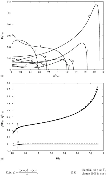
FIG. 4. The electric parameters for a core-shell droplet with⑀in= 3,⑀out= 2, ⑀sur= 1, ␴in=␴out= 33.72s−1= 3.75

⫻10−9_{S / m, attached to a nozzle} sub-jected to an electric field with BoE

Eq.共39兲numerically for E_⬁⫽0 we in fact find the solution as a sum

q=q1+qnet,0, 共40兲

where only q1 is the particular solution corresponding to a

given nonzero E_⬁ we are searching for. To exclude qnet,0,

note thatq1共−z兲= −q1共z兲, wherezis the vertical coordinate of

a point on the surface ⌫˜out,sur, since it corresponds to zero

total charge on the closed surface 共real and mirror image兲. On the other hand,qnet,0共−z兲=qnet,0共z兲. Therefore,q1 can be

found as

q₁=1₂关q共z兲−q共−z兲兴. 共41兲

The electric stress tensor in共4兲becomes␴_␣␤= 2␲q₁2␦_␣␤. The reduction of all the surface integrals in the axisym-metric case is described in detail in Ref. 20. The problem

then becomes effectively one-dimensional and the kernels G_␣␤,T_␣␤, and Kcan be expressed in terms of complete el-liptical integrals.

The time stepping dependence of the results was checked and found to be negligibly small.

V. EXPERIMENTAL SETUP

[image:7.612.53.558.48.451.2]

The experimental setup共Fig. 3兲permitted observation of the compound droplet evolution under conditions close to those implemented for the numerical simulations. Core-shell droplets共i兲of two different polymer solutions were formed at the end of two concentric needles. The position of the inner 共core兲 needle relative to the outer 共shell兲 needle was adjustable, and the protrusion varied from 0 to 0.42 mm. The shell solution inlet was connected to a high-voltage power supply 共HVPS兲 共ii兲 with variable voltage V = 11 to 15.57 kV. The voltage was turned on immediately

when the well-defined near-spherical outer surface and inner interface were observed 共t= 0兲. The numerical results dis-cussed below showed that the electric conductivity of both solutions was sufficiently high to allow all charges to migrate to the free surface of the outer fluid共shell兲over a short time interval compared to the characteristic time of droplet evo-lution. Thus both solutions were effectively equipotential al-most throughout the experiment. A grounded metal disk共iv兲, of radiusad= 5.75 cm, was placed 16 cm below the droplet, acting as a counterelectrode. The evolution process was im-aged with an electronic camera 共v兲 共MotionScope Redlake Imaging Corporation兲 actuated 共iii兲 synchronously with the application of high voltage to allow full temporal coverage of the evolution process. The camera was equipped with a 70– 180 mm, f/4.5 zoom lens. Its speed was 500 f.p.s. and the exposure time was 0.1 ms. A light source共vi兲 共halogen lamp, 500 W兲and diffuser共vii兲were placed behind the drop-let in line with the camera. The image processing was done using the Matlab image processing toolbox. The polymers used were polymethyl methacrylate 共PMMA兲 of molecular weightMw= 996 000 g mol−1共Aldrich兲and polyacrylonitrile

共PAN兲of molecular weightMw= 150 000 g mol−1共Scientific Polymer Products, Inc.兲. The solvent used was N, N-dimethyl formamide 共DMF兲 共Gadot lab. supplies兲. Three compositions were prepared: 共a兲 12 wt. % PAN in DMF 共shell solution兲, 共b兲 14 wt. % PMMA in DMF 共core solution I兲,共c兲18 wt. % PMMA in DMF 共core solution II兲. Tests were made with solutions共a兲and共b兲as the first set and

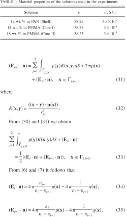
共a兲 and共c兲as the second set. Malachite green was added to the core solution to render it distinguishable from its shell counterpart. The permittivity and conductivity of the solu-tions are given in Table I. The surface tension of DMF at 25 ° C is ␥out,sur= 35.2 g / s2. According to Ref. 24, surface

tension of polymer solutions used in electrospinning is close to that of their solvents. Therefore, that value of␥out,surwas

used in the calculations in the present work. Zero-shear vis-cosity of the shell solution was measured using a Couette programmable viscometer Brookfield DV−II+. The result was in the range 40–⬃102P. For the core solution the same viscometer revealed the values of zero-shear viscosities in the range ⬃100– 400 P. The results should be considered only as an order of magnitude estimates due to the inaccura-cies typically involved in zero-shear viscosity measurements using the above-mentioned viscometer.19 Also, possible shear-thinning共non-Newtonian兲effects and the effect of sol-vent evaporation on the viscosity values cannot be excluded during droplet evolution.

VI. RESULTS AND DISCUSSION

For comparison with the experimental data, the follow-ing parameters were used: ␮in= 176 P, ␮out= 70.4 P 共based

on the experimental estimates兲, ␮sur= 0, ␮in/␮out= 2.5,

␥in,out/␥out,sur= 0, ␥out,sur= 35.2 g / s2 with core and shell

nozzle radii rin= 0.03471 cm, rout= 0.089 cm, respectively;

rin/rout= 0.39. The flow rates were taken asQ1= 0.05 ml/ h in

the core and Q2= 0.6 ml/ h in the shell. In addition, in the

[image:8.612.51.300.45.663.2]

model calculations in the framework of the leaky dielectric model the following parameters were used: ⑀in= 3, ⑀out= 2,

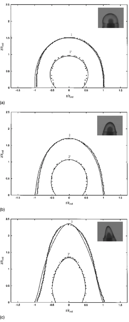
FIG. 6. Measured and predicted shapes of the core and shell interfaces at different time moments:共a兲1 and 1⬘−t= 0.2 s,共b兲2 and 2⬘−t= 0.28 s,共c兲3 and 3⬘−t= 0.4 s. The calculated shapes are plotted by solid lines, the experi-mental ones by symbols. The numerals for the shell have no primes, those for the core have primes. On the left-hand side the values ofr/a0are arti-ficially made negative. The inserts show the photographs used to acquire the experimental data presented by symbols in the main frames. BoE= 5.6,Q1 = 0.05 ml/ h, Q2= 1 ml/ h. No protrusion of the core nozzle,zp= 0. Core,

⑀sur= 1, ␴in=␴out= 33.72 s−1= 3.75⫻10−9 S / m. Comparing

[image:9.612.51.296.46.643.2]

these values with those listed in Table I, one can see that in the model calculations a much less conducting liquid was considered. Nevertheless, as is shown below, even this low-conducting liquid approached very rapidly to the behavior of a perfect conductor under the present conditions. In Fig. 4 several electric parameters are predicted for the core-shell drop attached to the nozzle共cf. Fig. 2兲at BoE= 7.2共the basic case, corresponding to the experimental value of the poten-tial dropV= 11 kV兲. As was explained in Ref. 19, the correct estimate of the electric field isE_⬁⬃2V/共␲·L兲, whereLis of the order of the shell-needle radius共the outer electrode used

FIG. 7. The tip heights, normalized byr_out, versus time for core nozzle protrusion outside the shell nozzle byzp= 0.042 cm;zp/rout= 0.47. Core, 18 wt. % PMMA; shell, 12 wt. % PAN.共a兲V= 11 kV,L= 0.39 cm, BoE= 9,

Q2= 1 ml/ h; the shell jetting time tsj= 0.352 s. 共b兲 V= 15.75 kV, L = 0.50 cm, BoE= 11.5, Q2= 1 ml/ h; tsj= 0.262 s. 共c兲 V= 15.75 kV, L = 0.48 cm, BoE= 12, Q2= 1 ml/ h; tsj= 0.27 s. In all cases Q1= 0.05 ml/ h. Error bars for the experimental data corresponding to the outer surface and the interface are shown. The predictions are shown by the dashed line共for the outer surface兲and the solid line共for the interface兲. The corresponding experimental data are shown by symbols.

[image:9.612.374.499.48.532.2]

in the experiment兲. Using it and the value of BoE, we obtain L= 0.44 cm, which is in fact close to the order of the needle radius used in the experiment. The distribution of the tangen-tial components of the electric field over the outer free sur-face and the intersur-face at some time moments is shown in Fig. 4共a兲. In particular, it is seen that initially the maximal values of these components are reached near the contact lines共close toz= 0兲; then they decrease in time rather rapidly, even with the moderate conductivity values taken here. For time mo-ments close to the emergence of jetting, the trend changes and the tangential field strength begins to increase both at the free surface and the interface, whereas the maxima are

reached near the tip关at z/r_out⯝1.6 to 1.9 for t/t₀= 1.81 in Fig. 4共a兲兴. The value ofE_␶near the tip increases rapidly with time, indicating that the electrical properties of the polymer solution 共its finite conductivity and the permittivity value兲 become important near the shell tip when the jet emerges. Both the free and overall charges,q and ␳, at the interface are also close to zero 共because of the screening effect兲, as curves 1

⬘

and 2

⬘

in Fig. 4共b兲show. On the other hand, both charges at the free surface关curves 1 and 2 in Fig. 4共b兲兴 are quite significant and begin to increase at a very high rate as the stretching process sets in. The free charge density ap-proaches that of the overall charge very rapidly, which

mani-FIG. 9. Core-shell droplet for different protrusionszp. ␮in/␮out= 5, rin/rout= 0.35, ␥in,out/␥out,sur= 0.8, Q1 = 0.07 ml/ h,Q2= 0.14 ml/ h and BoE= 10. In共a兲–共c兲the

[image:10.612.55.362.43.578.2]

fests the fact that the droplet bulk can, in fact, be considered as a conductor up to the jet formation. Therefore, even the leaky dielectric of the model fluid considered, which was much less conductive than the solutions in the experiments, approached very rapidly to the behavior of a perfect conduc-tor. Therefore, in all subsequent calculations the core and shell fluids were taken as perfect conductors from the very beginning up to the jet formation, which significantly simpli-fies the simulations.

In Fig. 5 the measured and calculated positions of the core and shell tips are compared for the case when the two nozzles face the same front line 共as in Fig. 4兲. Here and hereinafter the parameters used have the values listed at the beginning of the present section共called the basic case兲, ex-cept those given in the figure captions. In all cases jetting sets in and core-shell jets emerge, which was confirmed by the analysis of the as-spun nanofibers. The general agree-ment between the predicted and recorded droplet evolutions in the experiments is rather good. The overall shapes of the predicted and measured interfaces are also in satisfactory agreement共cf. Fig. 6兲.

As was explained above, in the present case practically all charges accumulate very rapidly at the outer surface of the shell fluid共that of the droplet兲, so that the electric force acted only on the free surface. Also, the volumetric flow rate in the core,Q₁, was always significantly lower than that in the shell,Q2. Therefore, the core could be entrained into the

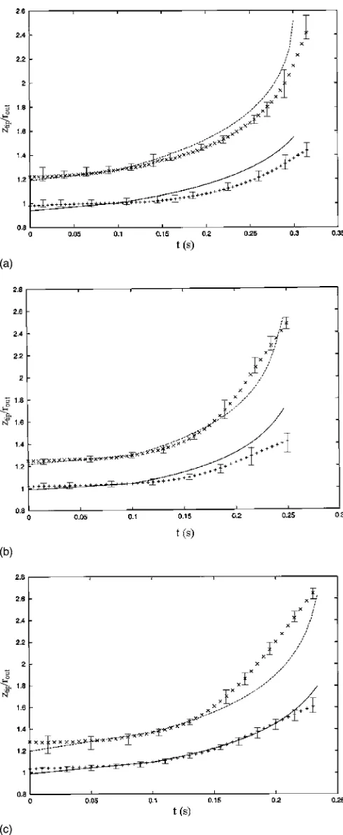
emerging jet only by the viscous forces generated in the shell. As the core fluid was 2.5 times more viscous than that of the shell, the entrainment effect seen in Fig. 5 was rather slow even though the interfacial tension共which could ham-per the entrainment兲 was practically zero. As a possible means of enhancing the entrainment effect, extension of the core nozzle outside the shell nozzle was considered. In these cases, as in the experiments, the vertical protrusion was taken to bezp= 0.042 cm共note that in Figs. 3–6zp= 0兲. The numerical results for these cases compared against the ex-perimental data in Fig. 7. Referring to Fig. 5, one can con-clude that entrainment was significantly improved for

protru-sion of about several tens percent ofr_out. The experimental results of the present work, as well as those of Ref. 11, con-firm this conclusion and show that core-shell nanofibers, do indeed form.

It is difficult to reach a definite positive answer to the question whether the core liquid has been entrained into the emerging shell jet, both by the experimental and numerical means. The electronic camera does not allow recording of the evolution of the core interface after the shell jetting has begun. That is the reason that film recording was terminated as the shell jetting set in Figs. 5 and 7. Also, as the shell jetting sets in, stretching of the surfaces becomes so strong that it is impossible to follow it numerically until a fully developed core jetting will appear. Therefore, judgment on formation of core-shell jet is based on the estimate whether the evolution of the core interface has not been saturated and become fully transient, as in Fig. 7, and to a less extent, in Fig. 5. The conclusions on formation of core-shell jets were corroborated by the analysis of the as-spun nanofibers.

Definite negative statements below, that the core is not entrained into the shell jet, will be based on purely numerical evidence that the rise of the interface tip has been fully satu-rated in spite of a significant rise of the shell tip.

It is emphasized that in comparably lower electric fields no jetting sets in either from the shell or the core tips, with or without protrusion. This conclusion is similar to that of Ref. 19 regarding the single-fluid case.

The cumulative information on the rise of the tips of the interface and the free surface for 0.5⬍␮in/␮out⬍100 and

rin/rout= 0.7, Q1= 0.07 ml/ h and Q2= 0.14 ml/ h, BoE= 10

shows that the electric field was sufficiently strong to induce jetting from the tip of the共outer兲free surface at all the vis-cosity ratios considered. However, at the given surface ten-sion ratio␥in,out/␥out,sur= 0.8, at a higher viscosity of the core

fluid共at 5艋␮in/␮out艋100兲the viscous forces generated by

[image:11.612.51.342.50.261.2]

the shell at the interface were too weak to create entrainment over a characteristic time comparable to that of jet emer-gence. In these cases no core-shell nanofibers were formed. Under lower electric field with BoE= 5, no jetting from the

interface tip set in even at very low core viscosity with

␮in/␮out= 0.1, with the same negative result as above.

How-ever, at higher flow rates Q1 and Q2 it proved possible to

achieve emergence of a core-shell jet. For example, under a relatively weak field 共BoE= 2兲 with Q1= 1.43 ml/ h and Q2

= 4.3 ml/ h, at small values of the viscosity ratio ␮in/␮out

= 0.01, the low-viscosity core fluid moved in both the axial and the radial directions, which led to significant swelling of the inner drop at the stage of formation of a core-shell jet关cf. Fig. 8共a兲兴. As the ratio␮in/␮outwas increased to 10 with the

other parameters fixed, the radial swelling decreased and the core fluid was entrained much faster into the jet 关cf. Fig. 8共b兲兴. Note, that in the absence of the electric field 共BoE = 0兲in the caseQ2⬎Q1the outer surface of the shell droplet

never acquires the shape of the rapidly thinning jet.

Some additional results on the effect of the protrusion are shown in Fig. 9, which refers to a highly viscous core fluid 共␮in/␮out= 5兲 and relatively high interfacial tension

共␥in,out/␥out,sur= 0.8兲, with rin/rout= 0.35, and BoE= 10. The

protrusion varied in the rangezp= 0.1 to 0.6. The results in-dicate that under the above field the entrainment of the core tip became significant共i.e., a compound jet was formed兲only at zp= 0.5, while at zp⬍0.5 and zp⬎0.6 it was practically absent. Jet formation from the outer tip was slowed down as the protrusion was increased, due to the viscous stresses im-posed on the outer fluid from the protruding nozzle surface and by the inner fluid. Jetting of the outer fluid set in at the outer tip at all protrusions except for the largestzp= 0.6, in which case it originated at some radial position on the outer drop surface 关cf. Fig. 9共c兲兴. In the present axisymmetric simulations this corresponds to corona-like jetting of the outer fluid; with nonaxisymmetric modes provided for, mul-tiple jetting from the surface of the outer drop can be pected. Such phenomena, have actually been observed in ex-periments in certain cases. The present results show that sideways jetting in core-shell co-electrospinning should not necessarily correspond to nonaxisymmetric perturbations of the electric field, but rather to strong interplay of the viscous effects related to the protruding core nozzle and to the outer fluid, and the electric Maxwell stresses.

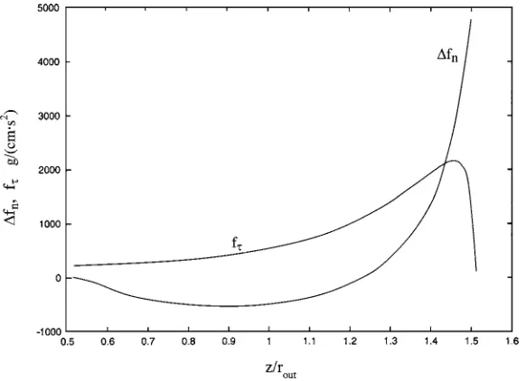
Figure 10 shows the distributions of the normal and tan-gential tractions per unit surface area of the core-shell inter-face in the droplet corresponding to case共c兲in Fig. 7. The relevant time moment共t/t0= 1.16兲is rather close to the onset

of jetting at the outer tip共t/t0= 1.31 in this case兲. It is seen

that the normal tractions increased dramatically close to the interface tip共atz/rout⯝1.5兲, whereas the shear stresses

pos-sess a maximum close to it, after which they drop and ap-proach zero at the tip. Similar data can be used to estimate the stress level experienced by viruses, bacteria, DNA mol-ecules, drugs, chromophores, enzymes dissolved in polymer solutions prior to encapsulation in nanofibers via co-electrospinning.25

VII. CONCLUSION

In sufficiently strong electric fields, jetting sets in at the tip of core-shell compound共two-fluid兲 droplets. This, how-ever, does not necessarily result in entrainment of the core

fluid and formation of a core-shell jet. As both the theoretical and experimental results of the present work show, formation of core-shell jets and nanofibers via co-electrospinning in the parameter range considered is greatly facilitated when the core nozzle protrudes outside the shell nozzle by around 0.5 of its radius共rout兲. At protrusions close to 0.6routtip jetting of

the shell fluid is replaced by a corona-like effect which leads to emergence of multiple jets, typically unstable in the ex-periments. Accordingly, the optimal protrusion for core-shell nanofiber formation, with the other parameters described in the text, is aboutzp= 0.5rout. The stress level at the interface

in the core-shell droplet before formation of the nanofibers is predicted to be of the order of 5⫻103g /共cm s2兲. The value is relevant in assessing the viability of viruses, bacteria, DNA molecules and drugs to be encapsulated in co-electrospun nanofibers. It is of the order of 104g /共cm s2兲, the stress which can cause red blood cell damage.26 There-fore, such stresses can probably cause damage to some bac-teria.

ACKNOWLEDGMENTS

The authors gratefully acknowledge the financial support of the Volkswagen Stiftung. The technical assistance of R. Avrahami and E. Katz is appreciated.

1_{Z. Sun, E. Zussman, A. L. Yarin, J. H. Wendorff, and A. Greiner,}

“Com-pound core-shell polymer nanofibers by co-electrospinning,” Adv. Mater.

共Weinheim, Ger.兲 15, 1929共2003兲.

2_{D. Li and Y. Xia, “Direct fabrication of composite and ceramic hollow}

nanofibers by electrospinning,” Nano Lett. 4, 933共2004兲.

3_{D. Li and Y. Xia, “Electrospinning of nanofibers: reinventing the wheel?”}

Adv. Mater.共Weinheim, Ger.兲 16, 1151共2004兲.

4_{Y. Zhang, Z. M. Huang, X. Xu, C. T. Lim, and S. Ramakrishna,}

“Prepa-ration of core-shell structured PCL-r-gelatin bi-component nanofibers by coaxial electrospinning,” Chem. Mater. 16, 3406共2004兲.

5_{J. H. Yu, S. V. Fridrikh, and G. C. Rutledge, “Production of submicrometer}

diameter fibers by two-fluid electrospinning,” Adv. Mater. 共Weinheim, Ger.兲 16, 1562共2004兲.

6_{D. H. Reneker, A. L. Yarin, H. Fong, and S. Koombhongse, “Bending}

instability of electrically charged liquid jets of polymer solutions in elec-trospinning,” J. Appl. Phys. 87, 4531共2000兲.

7_{A. L. Yarin, S. Koombhongse, and D. H. Reneker, “Bending instability in}

electrospinning of nanofibers,” J. Appl. Phys. 89, 3018共2001兲. 8_{M. M. Hohman, M. Shin, G. Rutledge, and M. P. Brenner,}

“Electrospin-ning and electrically forced jets: I. Stability theory,” Phys. Fluids13, 2201

共2001兲.

9_{M. M. Hohman, M. Shin, G. Rutledge, and M. P. Brenner,}

“Electrospin-ning and electrically forced jets: II. Applications,” Phys. Fluids 13, 2221

共2001兲.

10_{D. Li, J. T. McCann, and Y. Xia, “Use of electrospinning to directly}

fabricate hollow nanofibers with functionalized inner and outer surfaces,” Small 1, 83共2005兲.

11_{E. Zussman, A. L. Yarin, A. V. Bazilevsky, R. Avrahami, and M. Feldman,}

“Electrospun polyacrylonitrile/poly共methyl methacrylate兲-derived turbos-tratic carbon micro-/nanotubes,” Adv. Mater.共Weinheim, Ger.兲 18, 348

共2006兲.

12_{F. Li, X. Y. Yin, and X. Z. Yin, “Linear instability analysis of an electrified}

coaxial jet,” Phys. Fluids 17, 077104共2005兲.

13_{S. Ramakrishna, K. Fujihara, W. E. Teo, T. C. Lim, and Z. Ma, The}

Introduction to Electrospinning of Nanofibers 共World Scientific,

Sin-gapore, 2005兲.

14_{D. H. Reneker, A. L. Yarin, E. Zussman, and H. Xu, “Electrospinning of}

nanofibers from polymer solutions and melts,” in Advances in Applied

Mechanics, Vol. 41, edited by E. van der Giessen and H. Aref共Elsevier,

Oxford, 2006兲.

15_{J. D. Sherwood, “The deformation of a fluid drop in an electric field—A}

16_{X. Zhang and O. A. Basaran, “Dynamics of drop formation from a}

capil-lary in the presence of an electric field,” J. Fluid Mech.326, 239共1996兲. 17_{P. K. Notz and O. A. Basaran, “Dynamics of drop formation in an electric}

field,” J. Colloid Interface Sci. 213, 218共1999兲.

18_{V. G. Suvorov and E. A. Litvinov, “Dynamic Taylor cone formation on}

liquid metal surface: numerical modeling,” J. Phys. D 33, 1245共2000兲. 19_{S. N. Reznik, A. L. Yarin, A. Theron, and E. Zussman, “Transient and}

steady shapes of droplets attached to a surface in a strong electric field,” J. Fluid Mech.516, 349共2004兲.

20_{A. A. Becker,The Boundary Element Method in Engineering. A Complete}

Course共McGraw-Hill, New York, 1992兲.

21_{C. Pozrikidis,Boundary Integral and Singularity Methods for Linearized}

Viscous Flow共Cambridge University Press, Cambridge, 1992兲.

22_{D. A. Saville, “Electrohydrodynamics: The Taylor-Melcher leaky}

dielec-tric model,” Annu. Rev. Fluid Mech. 29, 27共1997兲.

23_{V. S. Vladimirov,Equations of Mathematical Physics共Nauka, Moscow,} 1988兲, in Russian.

24_{S. A. Theron, E. Zussman, and A. L. Yarin, “Experimental investigation of}

the governing parameters in the electrospinning of polymer solutions,” Polymer 45, 2017共2004兲.

25_{A. Greiner, J. H. Wendorff, A. L. Yarin, and E. Zussman, “Biohybrid}

nanosystems with polymer nanofibers and nanotubes,” Applied Microbi-ology and BiotechnMicrobi-ology共in press兲.

26_{S. Deutsch, J. M. Tarbell, K. B. Manning, G. Rosenberg, and A. A.}