Automatic detection of ionospheric Alfvén resonances using signal and image processing techniques

www.ann-geophys.net/32/951/2014/ doi:10.5194/angeo-32-951-2014

© Author(s) 2014. CC Attribution 3.0 License.

Automatic detection of ionospheric Alfvén resonances using signal

and image processing techniques

C. D. Beggan

British Geological Survey, West Mains Road, Edinburgh, EH9 3LA, UK

Correspondence to: C. D. Beggan ([email protected])

Received: 6 April 2014 – Revised: 3 July 2014 – Accepted: 4 July 2014 – Published: 12 August 2014

Abstract. Induction coils permit the measurement of small and very rapid changes of the magnetic field. A new set of induction coils in the UK (at L=3.2) record magnetic field changes over an effective frequency range of 0.1– 40 Hz, encompassing phenomena such as the Schumann res-onances, magnetospheric pulsations and ionospheric Alfvén resonances (IARs). The IARs typically manifest themselves as a series of spectral resonance structures (SRSs) within the 1–10 Hz frequency range, usually appearing as fine bands or fringes in spectrogram plots and occurring almost daily dur-ing local night-time, disappeardur-ing durdur-ing the daylight hours. The behaviour of the occurrence in frequency (f) and the difference in frequency between fringes (1f) varies through-out the year. In order to quantify the daily, seasonal and an-nual changes of the SRSs, we developed a new method based on signal and image processing techniques to identify the fringes and to quantify the values off,1fand other relevant parameters in the data set. The technique is relatively robust to noise though requires tuning of threshold parameters. We analyse 18 months of induction coil data to demonstrate the utility of the method.

Keywords. Ionosphere (mid-latitude ionosphere; wave propagation; instruments and techniques)

1 Introduction

Spectral resonance structures (SRSs) are a type of extremely low frequency magnetic field phenomena detectable in the 0.5–10 Hz region of the magnetic field spectrum. Their ori-gin is attributed to the occurrence of ionospheric Alfvén resonances (IARs) between the E and F2 region layers of the upper atmosphere. The theoretical framework for IARs was originally posited by Polyakov and Rapoport (1981),

and their existence was confirmed some years later by ex-perimental detection in magnetic induction search coil data (e.g. Belyaev et al., 1989, 1990). Further theoretical mod-els have been developed (e.g. Lysak, 1993; Bösinger et al., 2009) to explain the phenomenon, and experimental work has provided evidence for their occurrence at low (Bösinger et al., 2002), middle (Kulak et al., 1999; Hebden et al., 2005) and high latitudes (Belyaev et al., 1999; Yahnin et al., 2003; Molchanov et al., 2004) in the Northern Hemisphere. Other researchers have shown SRSs are present in the Southern Hemisphere; for example, Yaun (2011) investigated SRSs measured at Halley Bay in Antarctica.

IARs are thought to arise from the partial reflection of magnetohydrodynamic Alfvén waves in the ionosphere, ex-cited along magnetic field lines by the leakage of electric fields associated with terrestrial lightning activity (Greifinger and Greifinger, 1968; Fukunishi et al., 1996; Füllekrug et al., 1998). The waves reflect off the “walls” of the E region and F2 region where the gradients of electron density reach a maximum. This partial reflection sets up a series of resonant frequencies along the field lines, giving rise to between 2 and 12 harmonics (the so-called SRS). The SRSs are visible as a series of fringes in dynamic spectrograms of the magnetic field rate of change.

There are several parameters which can be observed from the SRSs which allow us to probe conditions within the iono-sphere, but the primary one is the frequency interval (1f) between spectral lines. This parameter can be used to deter-mine length interval of the cavity if the corresponding foF2 values are available (e.g. Yahnin et al., 2003). From this other parameters such as the Alfvén velocity can be estimated.

visual identification to produce values of occurrence rate and frequency interval or scale over a 3-year period from an in-strument in Sodankylä, Finland. A combination of a manual point-and-click method and a semi-automatic method using fast Fourier transforms was applied by Hebden et al. (2005) to obtain key parameters, again from the Sodankylä data set. A paper by Odzimek et al. (2006) describes a semi-automated approach to capturing1f using Bessel function fitting with a data set recorded in Poland. More recently, Yaun (2011) used a smoothing and sine curve fitting method to identify the values of the frequency interval in the afore-mentioned Sodankylä data set. However, none of the meth-ods are fully automated, and all rely on some form of manual intervention.

In this study, we examine the use of a combination of signal and image processing techniques to identify the oc-currence and properties of SRS fringes in spectral data. In Sect. 2 we describe the data used showing examples of the spectral features of interest, and detail the methodology used for automatic detection. Section 3 shows the results of au-tomated processing of 18 months of data available from the UK observatory. We discuss the results in Sect. 4.

2 Data and methodology

In June 2012, the British Geological Survey (BGS) Ge-omagnetism team installed two horizontal high-frequency (100 Hz) induction coil magnetometers at the Eskdalemuir Observatory (55.3◦N, 3.2◦W;L=3.2), in the Scottish Bor-ders of the United Kingdom. The Eskdalemuir Observatory is one of the longest running geophysical sites in the UK (be-ginning operation in 1908) and is located in a rural valley with a generally quiet magnetic environment.

The instrumentation consists of two refurbished CM11-E induction coil magnetometers, north–south and east–west orientated, connected to a 24 bit Guralp digitiser. The digi-tiser converts the output signal from the coils for wired trans-mission to a logger located in a vault approximately 150 m from the coils. The data are recorded at 100 Hz by an on-site computer where they are collated into hourly files. The data are automatically collected from Eskdalemuir once per hour and permanently stored on the BGS network. Daily pro-cessing produces a set of spectrograph images for display on the BGS Geomagnetism website1. Since September 2012 the system has run almost continuously, losing only around 20 days of data (e.g. due to computer issues or component failure).

2.1 Visualising the SRSs

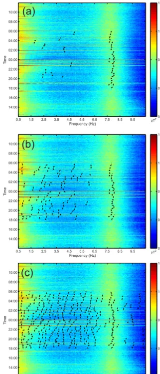
The SRSs appear as a set of fringes in time–frequency plots (i.e. spectrograms). Figure 1 shows three examples of spec-trograms computed from the coil measurements which show

1_{http://www.geomag.bgs.ac.uk/research/inductioncoils.html}

Frequency (Hz)

Ti

me

0.5 1.5 2.5 3.5 4.5 5.5 6.5 7.5 8.5 9.5 14:00

16:00 18:00 20:00 22:00 00:00 02:00 04:00 06:00 08:00 10:00

pT20.001 0.01 0.1 1 10

Frequency (Hz)

Ti

me

0.5 1.5 2.5 3.5 4.5 5.5 6.5 7.5 8.5 9.5 14:00

16:00 18:00 20:00 22:00 00:00 02:00 04:00 06:00 08:00 10:00

pT20.001 0.01 0.1 1 10

Frequency (Hz)

Ti

me

0.5 1.5 2.5 3.5 4.5 5.5 6.5 7.5 8.5 9.5 14:00

16:00 18:00 20:00 22:00 00:00 02:00 04:00 06:00 08:00 10:00

pT20.001 0.01 0.1 1 10

(a)

(b)

(c)

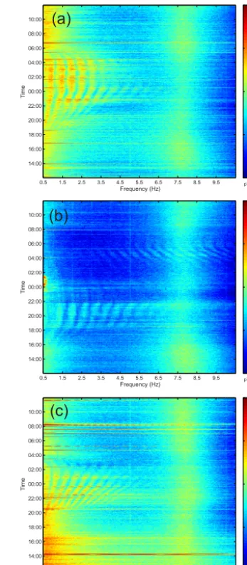
Figure 1. Example spectrograms with clearly visible spectral reso-nance structures from (a) 23–24 September 2012: a typical “good” day with clearly visible SRSs; (b) 11–12 January 2013: SRSs

visi-ble at>7 Hz between 03:00 and 06:00; (c) 29–30 July 2013:

non-linear fan-shaped SRSs.

clear SRSs. To obtain these plots, the raw digitiser data are bandpass filtered between 0.5 and 10 Hz using a five-pole Butterworth filter in the time domain. This is primarily to re-move the influence of longer period variations in the data, as the instrument level drifts with the general background mag-netic field over a day. As the field is sampled at 100 Hz, there are no issues with aliasing or loss of power at these frequen-cies.

A spectrogram is created by stacking the outputs of 862 1-D FFT traces into a 2-D matrix.

The SRSs show a large variety of dynamic behaviour. On a typical day, they usually start as a single low frequency around the onset of local night-time before bifurcating into 5–10 separate fringes, increasing in frequency until around midnight (Fig. 1a). The fringes also widen in frequency until midnight before fading around the beginning of daylight. Oc-casionally, the fringes decrease in frequency slightly around 03:00 UT before eventually fading. No fringes are detected during daylight hours.

On rare occasions the SRSs can be seen at frequencies higher than the first Schumann resonance at≈8 Hz (Fig. 1b). Other behaviours such as non-linearly spaced1f occasion-ally appear (Fig. 1c). The spectrograms also show Pc1 pulsa-tions (around 00:00–02:00 UT in Fig. 1b) and traces of hori-zontal broadband noise from “local” lightning storms within 2000 km (around 14:00 UT in Fig. 1c). The first Schumann resonance shows the typical diurnal variation related to the progressive triggering of tropical thunderstorms across the equatorial continental regions (i.e. Africa, America, Asia) as the Earth rotates. Despite being in an electrically and mag-netically quiet region of the UK, there are still effects from harmonics of man-made noise, visible as thin vertical lines on the integer-valued frequencies (e.g. 1, 2, 3 Hz in Fig. 1b).

2.2 Method

We wish to automatically detect the position of the SRS fringes. The method can be divided into two parts. The first

signal processing part approximately follows the methods of

Odzimek et al. (2006) and Yaun (2011) to identify the SRS peak frequency within each FFT trace while the second part involves the use of image processing to link the individual peaks together and discern the continuous SRSs. The method is fully automatic once some thresholds have been set from inspection. As with any method, there is a trade-off to be made between detection of signal and sensitivity to noise.

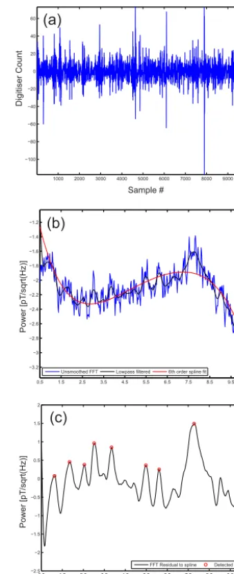
We choose 14–15 February 2014 to demonstrate the method as it is a “good” day with low Kp and no local light-ning activity or noise. The processing method starts with detrending and filtering the raw digitiser data from 0.5 to 10 Hz using a Butterworth five-pole filter in the time do-main as shown in Fig. 2a. A series of FFTs are computed using the Welch method with 100 s of filtered data to pro-duce 862 1-D spectra plots per day (from which the spec-trograms are produced). The individual spectra are converted to SI units using the instrument response and digitiser cali-bration values (Fig. 2b). The smoothed non-stationary IAR peaks in each time slice are identified using the residuals from a best-fit sixth-order spline fit to remove the background trend (Fig. 2b). The size of the smoothing window depends on the number of samples per Hz. For this data set, a window of 14 samples (0.3 Hz) wide is sufficient to smooth the data.

1000 2000 3000 4000 5000 6000 7000 8000 9000 10000

−100 −80

−60

−40

−20 0 20 40 60

Digitiser Count

Sample #

(a)

0.5 1.5 2.5 3.5 4.5 5.5 6.5 7.5 8.5 9.5

−2.5 −2 −1.5 −1 −0.5

0 0.5 1 1.5 2

Freq [Hz]

FFT Residual to spline Detected Peaks

(c)

Freq [Hz]

Power [p

T/

sqrt(Hz)

]

0.5 1.5 2.5 3.5 4.5 5.5 6.5 7.5 8.5 9.5

−3.2 −3 −2.8 −2.6 −2.4 −2.2 −2 −1.8 −1.6 −1.4 −1.2

Unsmoothed FFT Lowpassfiltered 6th order spline fit

Power [p

T/

sqrt(Hz)

]

(b)

Figure 2. Signal processing protocol for identifying SRS peaks for 14–15 February 2014. See text for details. (a) De-trending and fil-tering of 100 s of 100 Hz raw digitiser data. (b) FFT of 100 s of Hanning-windowed data (blue), 14-point running average smoothed FFT data (red) and sixth-order spline background (black); (c) spline background removed from smoothed FFT with main peaks identi-fied (circles).

(b)

Freq [Hz]

Ti

me

0.5 1.5 2.5 3.5 4.5 5.5 6.5 7.5 8.5 9.5 14:00

16:00 18:00 20:00 22:00 00:00 02:00 04:00 06:00 08:00 10:00

pT20.001

0.01 0.1 1 10

(d)

Freq [Hz]

Ti

me

0.5 1.5 2.5 3.5 4.5 5.5 6.5 7.5 8.5 9.5 20:00

22:00 00:00 02:00 04:00 06:00

(c) (a)

Ti

me

Ti

me

14:00 14:00

16:00 16:00

18:00 18:00

20:00 20:00

22:00 22:00

00:00 00:00

02:00 02:00

04:00 04:00

06:00 06:00

08:00 08:00

10:00 10:00

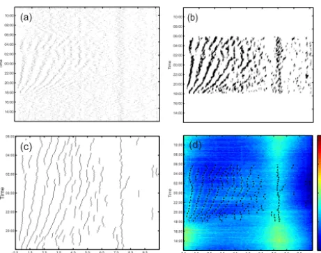
Figure 3. Image processing protocol for identifying continuous SRS features for 14–15 February 2014. See text for details. (a) Im-age of peak “spots” identified in the smoothed FFT data; (b) di-lation, erosion and bridging of “spots” image; (c) computation of weighted mean position of SRSs; (d) superposition of SRS peak locations with spectrogram. Features outside 18:00 and 06:00 are ignored in (b), (c), and (d).

rate which gives a frequency resolution of 1/40.96 Hz. The bandwidth of interest is between 0.5 and 10.5 Hz, meaning that the required number of points from each FFT is 410. Thus, the output “spots” image from the signal processing part has a size of 862 rows by 410 columns. This is used in the next stage which applies standard image processing tech-niques to link the “spots” together.

The next stage attempts to identify continuous SRS peaks by using standard image processing techniques (e.g. Kong and Rosenfeld, 1996; Gonzales and Woods, 2002). Figure 3a shows the input “spots” matrix to the image processing step. We wish to link together the continuous peaks but reject noise or sporadic peaks as best as possible. The “spots” im-ages are first “dilated” by an extrusion of 15 pixels in the vertical direction and then “eroded” by a line reduction of 3 pixels in the horizontal direction. The two threshold values for the size of the dilation and the severity of the erosion were chosen from experimentation and relate mainly to the fre-quency and time resolution, as well as the general noise lev-els. Pixels that are touching after these operations are classed as been “connected” and are joined using the 2-D “bridge” morphological operator which dilates the connection. These regions are further dilated again to give the approximate po-sition of the SRSs (Fig. 3b).

Next, the image in Fig. 3b and the original spectrogram are passed into the regionprops function in Matlab to deter-mine the area and bounding box for each distinct region. The

regionprops function works on binary images, splitting the

connected positive-valued regions into distinct labelled com-ponents before computing various spatial properties such as

2 4 6 8 10 12 14 0

0.05 0.1 0.15

0.2 Number of peaks

Occurence

2 4 6

0 0.01 0.02 0.03 0.04 0.05 0.06

0.07 Frequency of peaks

0 2 4 6

0 0.05 0.1 0.15 0.2 0.25 0.3

0.35 ∆ f of peaks

2 4 6 8 10 12 14 0

0.05 0.1 0.15 0.2

Occurence

Number 2 4 6

0 0.01 0.02 0.03 0.04 0.05 0.06 0.07

Frequency (Hz) 0 2 4 6

0 0.05 0.1 0.15 0.2 0.25 0.3 0.35

Frequency (Hz)

Figure 4. Histograms of the number of fringes (left), frequency

lo-cation (middle) and frequency interval (1f) (right) for all 525 days

(upper) and 152 selected “good” days (lower) from September 2012

to February 2014. Fringes withf >6.5 Hz are ignored.

the pixel area, the coordinates of the rectangular bounding box containing the region, the length of the perimeter and so on.

For this application, if the area of the detected region is less than 80 pixels, it is rejected and subsequently ignored. If the area is equal to or larger than 80 pixels, the bounding box is used to mask the spectrogram image and compute the weighted mean value of the pixels in that region of the spec-trogram. This identifies the positions of pixels with the max-imum amplitude in each row of the spectrogram matrix, and hence the peaks of the SRSs. These positions are shown in Fig. 3c. Values outside of local night-time (18:00–06:00) are ignored. Figure 3d shows the locations of the SRSs plotted onto the original spectrogram for the 14/15 February 2014. The positions of the SRSs can now be mapped as continuous lines throughout the spectrogram, and the relevant properties of interest can be derived from the data in the matrix shown in Fig. 3c.

The method is easy to implement and relatively quick to process, taking about 1 minute per day on a conventional desktop machine. In the next section, we show the results of applying the methodology to 18 months of induction coil data.

3 Results

20:00 22:00 00:00 02:00 04:00 0

0.5 1

1.5 Average Delta Freq for Oct 2012/3

Delta freq (Hz)

20:00 22:00 00:00 02:00 04:00 0

0.5 1

1.5 Average Delta Freq for Nov 2012/3

Delta freq (Hz)

20:00 22:00 00:00 02:00 04:00 0

0.5 1

1.5 Average Delta Freq for Dec 2012/3

Delta freq (Hz)

20:00 22:00 00:00 02:00 04:00 0

0.5 1

1.5 Average Delta Freq for Jan 2013/4

Delta freq (Hz)

20:00 22:00 00:00 02:00 04:00 0

0.5 1

1.5 Average Delta Freq for Feb 2013/4

Delta freq (Hz)

20:00 22:00 00:00 02:00 04:00 0

0.5 1

1.5 Average Delta Freq for Mar 2013

Delta freq (Hz)

20:00 22:00 00:00 02:00 04:00 0

0.5 1

1.5 Average Delta Freq for Apr 2013

Delta freq (Hz)

20:00 22:00 00:00 02:00 04:00 0

0.5 1

1.5 Average Delta Freq for May 2013

Delta freq (Hz)

20:00 22:00 00:00 02:00 04:00 0

0.5 1

1.5 Average Delta Freq for Jun 2013

Delta freq (Hz)

20:00 22:00 00:00 02:00 04:00 0

0.5 1

1.5 Average Delta Freq for Jul 2013

Delta freq (Hz)

20:00 22:00 00:00 02:00 04:00 0

0.5 1

1.5 Average Delta Freq for Aug 2013

Delta freq (Hz)

20:00 22:00 00:00 02:00 04:00 0

0.5 1

1.5 Average Delta Freq for Sep 2013

Delta freq (Hz)

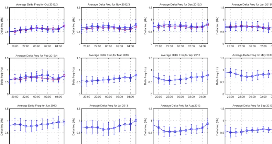
Figure 5. Plots of the hourly mean value of1f across each month for all 525 days from October 2012 to February 2014. Data for

Octo-ber 2012–SeptemOcto-ber 2013 (blue) and OctoOcto-ber 2013–February 2014 (red). Error bars show 1σ-level variation.

In addition, despite the site being relatively free of man-made interference, approximately 8 weeks show clear signs of con-tamination in the form of strong 1 Hz noise, which over-whelms the SRS features. To overcome these effects, the data set was split into “good” days by visual inspection to find 152 days where SRSs are clearly visible. As can be seen in Fig. 3d, the first Schumann resonance is also detected, so for our analysis, any SRSs detected above 6.5 Hz were ignored.

Figure 4 (upper) shows histograms of the number of fringes detected, the position in frequency in which the fringes occur and the 1f for all 525 days in the data set, while the lower panels show the results from the 152 selected “good” days. The histograms of the number of fringes sug-gest a modal value of 9 fringes for all the data, or 10 fringes for the selected data. Values of 1–2 fringes are most likely due to noise in the data sets. The frequency location of the fringes shows a preference between 0.5 and 4 Hz. SRSs oc-cur slightly less often at frequencies of 4–6.5 Hz. In the upper middle panel there are larger values at the integer Hz fre-quencies. These are related to periods when man-made noise is prevalent in the data set. The right-hand histograms show the value of1f across the data set. The modal value is be-tween 0.5 and 0.75 Hz in both the full and partial selections of the data. This agrees well with previous observations from Yahnin et al. (2003), for example.

Figures 5 and 6 show the results of dividing the1f data into the weighted average value per hour in UT for each of the 18 months. In Fig. 5 all the data were used, giving an equal number of data per month. In Fig. 6, the months are

shown individually as each contains a different number of “good” days. The error bars show the 1σ variation of the data.

The average value of1f varies seasonally. From Fig. 5,

1f is largest in Northern Hemisphere winter and smallest around the equinoxes. The error bars for the months of June and July are too large to make a definitive statement about the average value. Figure 6 shows a similar seasonal variation but suggests that1fis smallest at the summer solstice. Note the end points of the analysis (e.g. at the start or finish of local night-time) have the largest error bars – particularly during Northern Hemisphere summer.

Although an obvious visual daily variation is the increase off and1f over the period from evening to midnight often followed by a decrease before daytime, this trend does not appear to be consistent enough to be observed in the hourly UTC averages. We would expect to see a convex-upward set of lines in Figs. 5 and 6. However, this is not observed, sug-gesting that it does not occur often enough to influence the overall statistics.

4 Discussion

20:00 22:00 00:00 02:00 04:00 0

0.5 1

1.5Average Delta Freq for Sep−2012 #:4

Delta freq (Hz)

20:00 22:00 00:00 02:00 04:00 0

0.5 1

1.5Average Delta Freq for Oct−2012 #:13

Delta freq (Hz)

20:00 22:00 00:00 02:00 04:00 0

0.5 1

1.5Average Delta Freq for Nov−2012 #:8

Delta freq (Hz)

20:00 22:00 00:00 02:00 04:00 0

0.5 1

1.5Average Delta Freq for Dec−2012 #:5

Delta freq (Hz)

20:00 22:00 00:00 02:00 04:00 0

0.5 1

1.5Average Delta Freq for Jan−2013 #:9

Delta freq (Hz)

20:00 22:00 00:00 02:00 04:00 0

0.5 1

1.5Average Delta Freq for Feb−2013 #:4

Delta freq (Hz)

20:00 22:00 00:00 02:00 04:00 0

0.5 1

1.5Average Delta Freq for Mar−2013 #:10

Delta freq (Hz)

20:00 22:00 00:00 02:00 04:00 0

0.5 1

1.5Average Delta Freq forApr−2013 #:4

Delta freq (Hz)

20:00 22:00 00:00 02:00 04:00 0

0.5 1

1.5Average Delta Freq for May−2013 #:3

Delta freq (Hz)

20:00 22:00 00:00 02:00 04:00 0

0.5 1

1.5Average Delta Freq for Jun−2013 #:3

Delta freq (Hz)

20:00 22:00 00:00 02:00 04:00 0

0.5 1

1.5Average Delta Freq for Jul−2013 #:8

Delta freq (Hz)

20:00 22:00 00:00 02:00 04:00 0

0.5 1

1.5Average Delta Freq forAug−2013 #:11

Delta freq (Hz)

20:00 22:00 00:00 02:00 04:00 0

0.5 1

1.5Average Delta Freq for Sep−2013 #:18

Delta freq (Hz)

20:00 22:00 00:00 02:00 04:00 0

0.5 1

1.5Average Delta Freq for Oct−2013 #:14

Delta freq (Hz)

20:00 22:00 00:00 02:00 04:00 0

0.5 1

1.5Average Delta Freq for Nov−2013 #:12

Delta freq (Hz)

20:00 22:00 00:00 02:00 04:00 0

0.5 1

1.5Average Delta Freq for Dec−2013 #:6

Delta freq (Hz)

20:00 22:00 00:00 02:00 04:00 0

0.5 1

1.5Average Delta Freq for Jan−2014 #:10

Delta freq (Hz)

20:00 22:00 00:00 02:00 04:00 0

0.5 1

1.5Average Delta Freq for Feb−2014 #:7

Delta freq (Hz)

Figure 6. Plots of the hourly mean value of1ffor 152 selected “good” days in each month from September 2012 to February 2014. Error

bars show 1σ-level variation.

full solar cycle from 1985 to 1997. The variation of 1f

both over diurnal and seasonal timescales, which we show in Figs. 5 and 6, has been noted by many other studies. Yahnin et al. (2003) also showed very strong indication of solar cycle variation, which we cannot yet validate. It is in-teresting to note that, in the Yahnin et al. (2003) data set, the frequency scale fell to its lowest value around 0.5 Hz (their Fig. 2b) at the peak of the solar cycle. The data presented here have been collected during solar maximum (albeit a weak cycle) and have a similar average frequency scale. However, there may also be a latitudinal effect as the Eskdalemuir site is located further south atL=3.2 compared toL=5.2.

As with any signal or image processing technique, a trade-off exists between the sensitivity to signal and rejection of noise. The method is adept at detecting man-made interfer-ence, particularly linear features in the time–frequency plots. Figure 7 is an example of continuous noise detected on site for several weeks in May 2013, the cause of which is un-known. This type of interference accounts for the large val-ued bars in the integer frequency locations of the upper mid-dle histogram in Fig. 4. Excluding such data is the easiest method for reducing their effect in statistical analyses.

Detection of SRSs is also sensitive to the threshold value set in the peak finding algorithm. Lowering the threshold increases the number of “spots” for the image processing step but introduces further noise and spurious SRSs. Figure 8 shows the effect of changing the peak-finding threshold from a high threshold value of 0.5 (Fig. 8a), where the ratio of the maximum to minimum peak range is 0.5, through the

Frequency (Hz)

Time

0.5 1.5 2.5 3.5 4.5 5.5 6.5 7.5 8.5 9.5

14:00 16:00 18:00 20:00 22:00 00:00 02:00 04:00 06:00 08:00 10:00

pT20.001 0.01 0.1 1 10

Figure 7. Example spectrogram of data from 25 to 26 May 2013 with very strong contamination from man-made interference (verti-cal lines).

Frequency (Hz)

Ti

me

0.5 1.5 2.5 3.5 4.5 5.5 6.5 7.5 8.5 9.5 14:00

16:00 18:00 20:00 22:00 00:00 02:00 04:00 06:00 08:00 10:00

pT20.001 0.01 0.1 1 10 Frequency (Hz)

Ti

me

0.5 1.5 2.5 3.5 4.5 5.5 6.5 7.5 8.5 9.5 14:00

16:00 18:00 20:00 22:00 00:00 02:00 04:00 06:00 08:00 10:00

pT20.001 0.01 0.1 1 10

Frequency (Hz)

Ti

me

0.5 1.5 2.5 3.5 4.5 5.5 6.5 7.5 8.5 9.5 14:00

16:00 18:00 20:00 22:00 00:00 02:00 04:00 06:00 08:00 10:00

pT20.001 0.01 0.1 1 10 (a)

(b)

(c)

Figure 8. Example spectrogram 13–14 June 2013 with differ-ent threshold values used in the peak finding algorithm: (a) 0.5; (b) 0.25; (c) 0.1. See text for details.

Although SRSs occur occasionally at frequencies higher than 7 Hz, it is difficult to distinguish when they overlap with the first Schumann resonance between 7.5 and 8.5 Hz. The analysis deliberately ignores SRSs which occur at frequen-cies higher than the first Schumann resonance, as the detected features there are generally due to noise. Finally, the method, as currently implemented, is imperfect at capturing fine SRS (e.g. Bösinger et al., 2004) where1f <0.2 Hz – though such features are rarely present in our data set.

We note that the method can be modified to detect other features of interest in data presented in the form of spec-trogram by using a different bandpass filter and modifying the peak-finding threshold. For example, the method could be used to monitor the Schumann resonances or Pc1-type magnetosphere pulsations. The method can also be combined with other data sources such as the foF2 peak frequency from ionosonde data to infer near-real-time characteristics of the ionosphere.

5 Conclusions

We present an automatic method for detecting spectral res-onance structures (SRSs) within the 0.5–6.5 Hz frequency range of induction coil data. The method is based on a mix-ture of signal and image processing techniques and can be used to locate SRS features and to quantify values such as the frequency interval (1f) parameter in the data set. The technique is relatively robust to noise and works with low signal-to-noise ratio, though it does require user intervention to set a number of threshold values initially to suit the data set under investigation. We process 18 months of data to anal-yse the number of fringes, the occurrence location of SRSs in frequency and the frequency scale between fringes. These vary constantly throughout the year in a manner consistent with the results from previous studies. The method can also be applied to other phenomena of interest in the induction coil data such as detecting Schumann resonance properties or magnetospheric pulsations.

Acknowledgements. The author wishes to acknowledge the efforts of the BGS Geomagnetism engineering team in building, installing and maintaining the induction coil system at Eskdalemuir. The au-thor thanks Kittiphon Boonma for his assistance on an initial ver-sion of this research. This paper is published with the permisver-sion of the Director of the British Geological Survey (NERC).

Topical Editor S. Milan thanks two anonymous referees for their help in evaluating this paper.

References

Belyaev, P. P., Polyakov, C. V., Rapoport, V. O., and Trakhtengerts, V. Y.: Experimental studies of the spectral resonance structure of the atmospheric electromagnetic noise background within the range of short-period geomagnetic pulsations, Radiophys. Quan-tum El., 32, 491–501, doi:10.1007/BF01058169, 1989. Belyaev, P. P., Polyakov, S., Rapoport, V., and Trakhtengerts, V. Y.:

The ionospheric Alfvén resonator, J. Atmos. Terr. Phys., 52, 781– 788, doi:10.1016/0021-9169(90)90010-K, 1990.

Belyaev, P. P., Polyakov, S. V., Ermakova, E. N., and Isaev, S. V.: Experimental studies of the ionospheric Alfvén cavity using ob-servations of electromagnetic noise background over the solar cycle of 1985 to 1995, Radiophys. Quantum El., 40, 879–889, doi:10.1007/BF02676584, 1997.

Belyaev, P. P., Bösinger, T., Isaev, S., and Kangas, J.: First evidence at high latitudes for the ionospheric Alfvén resonator, J. Geo-phys. Res., 104, 4305–4317, doi:10.1029/1998JA900062, 1999. Bösinger, T., Haldoupis, C., Belyaev, P., Yakunin, M.,

Semen-ova, N., Demekhov, A., and Angelopoulos, V.: Spectral prop-erties of the ionospheric Alfvén resonator observed at a

low-latitude station (L=1.3), J. Geophys. Res., 107, 1281,

doi:10.1029/2001JA005076, 2002.

Bösinger, T., Demekhov, A., and Trakhtengerts, V.: Fine struc-ture in ionospheric Alfvén resonator spectra observed at

low latitude (L=1.3), Geophys. Res. Lett., 31, L11802,

Bösinger, T., Ermakova, E. N., Haldoupis, C., and Kotik, D. S.: Magnetic-inclination effects in the spectral resonance structure of the ionospheric Alfvén resonator, Ann. Geophys., 27, 1313– 1320, doi:10.5194/angeo-27-1313-2009, 2009.

Fukunishi, H., Takahashi, Y., Kubota, M., Sakanoi, K., Inan, U., and Lyons, W.: Elves: Lightning-induced transient luminous events in the lower ionosphere, Geophys. Res. Lett., 23, 2157–2160, doi:10.1029/96GL01979, 1996.

Füllekrug, M., Fraser-Smith, A. C., and Reising, S. C.: Ultra-slow tails of sprite-associated lightning flashes, Geophys. Res. Lett., 25, 3497–3500, doi:10.1029/98GL02590, 1998.

Gonzales, R. C. and Woods, R. E.: Digital Image Processing, 2nd Edn., Prentice Hall, 2002.

Greifinger, C. and Greifinger, P. S.: Theory of hydromagnetic propa-gation in the ionospheric waveguide, J. Geophys. Res., 73, 7473– 7490, doi:10.1029/JA073i023p07473, 1968.

Hebden, S. R., Robinson, T. R., Wright, D. M., Yeoman, T., Raita, T., and Bösinger, T.: A quantitative analysis of the diurnal evo-lution of Ionospheric Alfvén resonator magnetic resonance fea-tures and calculation of changing IAR parameters, Ann. Geo-phys., 23, 1711–1721, doi:10.5194/angeo-23-1711-2005, 2005. Kong, T. Y. and Rosenfeld, A.: Topological Algorithms for Digital

Image Processing, Elsevier Science, Inc., 1996.

Kulak, A., Maslanka, K., Michalec, A., and Zieba, S.: Observations of Alfvén ionospheric resonances on the Earth’s surface, Stud. Geophys. Geod., 43, 399–406, doi:10.1023/A:1023235219238, 1999.

Lysak, R. L.: Generalized model of the ionospheric Alfvén res-onator, Geophysical Monograph Series, 80, 121–128, 1993. Molchanov, O., Schekotov, A. Y., Fedorov, E., and Hayakawa,

M.: Ionospheric Alfvén resonance at middle latitudes: results of observations at Kamchatka, Phys. Chem. Earth, 29, 649–655, doi:10.1016/j.pce.2003.09.022, 2004.

Odzimek, A.: Numerical estimate of the spectral

res-onance structure frequency scale of natural ULF

magnetic field, Stud. Geophys. Geod., 48, 647–660,

doi:10.1023/B:SGEG.0000037476.82719.47, 2004.

Odzimek, A., Kułak, A., Michalec, A., and Kubisz, J.: An au-tomatic method to determine the frequency scale of the iono-spheric Alfvén resonator using data from Hylaty station, Poland, Ann. Geophys., 24, 2151–2158, doi:10.5194/angeo-24-2151-2006, 2006.

Polyakov, S. and Rapoport, V.: The Ionospheric Alfvén res-onator, Geomagn. Aeronomy, 21, 816–822, doi:10.1016/0021-9169(90)90010-K, 1981.

Yahnin, A. G., Semenova, N. V., Ostapenko, A. A., Kangas, J., Manninen, J., and Turunen, T.: Morphology of the spectral res-onance structure of the electromagnetic background noise in

the range of 0.1–4 Hz atL=5.2, Ann. Geophys., 21, 779–786,

doi:10.5194/angeo-21-779-2003, 2003.