www.geosci-model-dev.net/9/1423/2016/ doi:10.5194/gmd-9-1423-2016
© Author(s) 2016. CC Attribution 3.0 License.
Development and evaluation of CNRM Earth system model –
CNRM-ESM1
Roland Séférian1, Christine Delire1, Bertrand Decharme1, Aurore Voldoire1, David Salas y Melia1,
Matthieu Chevallier1, David Saint-Martin1, Olivier Aumont2, Jean-Christophe Calvet1, Dominique Carrer1, Hervé Douville1, Laurent Franchistéguy1, Emilie Joetzjer3, and Séphane Sénési1
1CNRM, Centre National de Recherches Météorologiques, Météo-France/CNRS, 42 Avenue Gaspard Coriolis,
31057 Toulouse, France
2Sorbonne Universités (UPMC, Univ Paris 06)-CNRS-IRD-MNHN, LOCEAN-IPSL Laboratory, 4 Place Jussieu,
75005 Paris, France
3Department of Ecology, Institute on Ecosystems, Montana State University, 111 AJM Johnson Hall, Bozeman,
Montana 59717, USA
Correspondence to: Roland Séférian ([email protected])
Received: 18 June 2015 – Published in Geosci. Model Dev. Discuss.: 22 July 2015 Revised: 27 February 2016 – Accepted: 29 March 2016 – Published: 19 April 2016
Abstract. We document the first version of the Centre Na-tional de Recherches Météorologiques Earth system model (CNRM-ESM1). This model is based on the physical core of the CNRM climate model version 5 (CNRM-CM5) model and employs the Interactions between Soil, Biosphere and Atmosphere (ISBA) and the Pelagic Interaction Scheme for Carbon and Ecosystem Studies (PISCES) as terrestrial and oceanic components of the global carbon cycle. We describe a preindustrial and 20th century climate simulation following the CMIP5 protocol. We detail how the various carbon reser-voirs were initialized and analyze the behavior of the car-bon cycle and its prominent physical drivers. Over the 1986– 2005 period, CNRM-ESM1 reproduces satisfactorily several aspects of the modern carbon cycle. On land, the model captures the carbon cycling through vegetation and soil, re-sulting in a net terrestrial carbon sink of 2.2 Pg C year−1. In the ocean, the large-scale distribution of hydrodynamical and biogeochemical tracers agrees with a modern climatol-ogy from the World Ocean Atlas. The combination of bi-ological and physical processes induces a net CO2 uptake of 1.7 Pg C year−1 that falls within the range of recent esti-mates. Our analysis shows that the atmospheric climate of CNRM-ESM1 compares well with that of CNRM-CM5. Bi-ases in precipitation and shortwave radiation over the tropics generate errors in gross primary productivity and ecosystem respiration. Compared to CNRM-CM5, the revised ocean–
sea ice coupling has modified the sea-ice cover and ocean ventilation, unrealistically strengthening the flow of North Atlantic deep water (26.1±2 Sv). It results in an accumu-lation of anthropogenic carbon in the deep ocean.
1 Introduction
Earth system models (ESMs) are now recognized as the cur-rent state-of-the-art models (IPCC, 2013), expanding the nu-merical representation of the climate system of the 4th As-sessment Report (IPCC, 2007). They enable the representa-tion of subtle nonlinear interacrepresenta-tions and feedbacks of dif-ferent magnitude and signs of various biogeochemical and biophysical processes with the climate system. The latter contribute, in addition to the atmospheric radiative proper-ties and global climate dynamics, to determining the Earth’s climate variability (Arora et al., 2013; Cox et al., 2000; Friedlingstein and Prentice, 2010; Schwinger et al., 2014; Wetzel et al., 2006).
primarily through their contribution to the concentration- and emission-driven experiments that compose CMIP5.
Even if the concept of Earth system modeling is being ex-tended to include further processes and reservoirs (e.g., nitro-gen cycle, aerosols) (Hajima et al., 2014), there are still large uncertainties in the representation of the carbon cycle and its interactions with climate (Anav et al., 2013a; Friedlingstein et al., 2013; Piao et al., 2013). To reduce them, there is a need for improvements of both physical and ecophysiological pa-rameterizations (Dalmonech et al., 2014), and for the de-velopment of observation-based methods to constrain model projections (Wenzel et al., 2014). But the reduction of car-bon cycle–climate uncertainties also requires a greater num-ber and diversity of ESMs. This path is promoted and fol-lowed by various international initiatives like the Global Car-bon Budget (http://www.globalcarCar-bonproject.org/) that se-quentially incorporate more and more models into their anal-yses (Le Quéré et al., 2013, 2015).
This article documents the first IPCC-class ESM devel-oped at Centre National de Recherches Météorologiques (CNRM) and provides a basic evaluation of the model’s skill. This model is based on the CNRM-CM5.1 climate model jointly developed by CNRM and Cerfacs (Centre Eu-ropéen de Recherche et de Formation Avancée en Calcul Scientifique), which has contributed to the 5th phase of the Coupled Model Intercomparison Project (CMIP5) (Voldoire et al., 2013). CNRM-CM5.1 did not include a representa-tion of the global carbon cycle but accounted for chemical– climate interactions with an interactive stratospheric chem-istry module (Cariolle and Teyssèdre, 2007). While this con-figuration of CNRM-CM5 contributed to the CMIP5 results publicly released, a first intermediate version of the CNRM ESM was developed with the inclusion of the marine bio-geochemistry model Pelagic Interaction Scheme for Carbon and Ecosystem Studies (PISCES) (Aumont and Bopp, 2006). This model version was evaluated against modern oceanic observations (Séférian et al., 2013) and employed in vari-ous studies (Frölicher et al., 2014; Laufkötter et al., 2015; Schwinger et al., 2014; Séférian et al., 2014).
A terrestrial carbon cycle module has been under develop-ment at CNRM since the 2000s (Calvet and Soussana, 2001; Calvet et al., 2008, 2004; Gibelin et al., 2008, 2006), but it has never been coupled to an atmosphere–ocean model. This carbon cycle module evolved from the physically based In-teractions between Soil, Biosphere and Atmosphere (ISBA) model (Noilhan and Mahfouf, 1996; Noilhan and Planton, 1989) and is able to simulate the surface carbon fluxes and the terrestrial carbon pools. The carbon fluxes module was extensively tested over France and Europe (Sarrat et al., 2007; Szczypta et al., 2012), and the carbon cycle module was tested for temperate and high-latitude regions (Gibelin et al., 2006, 2008) and was used more recently in studies of carbon cycling over the Amazon basin (Joetzjer et al., 2015, 2014), permafrost regions (Rawlins et al., 2015) and at global scale (Carrer et al., 2013b). In this work, this terrestrial
car-bon cycle module is coupled to a global climate model for the first time.
Here, we present a first evaluation of the CNRM-ESM1. In Sect. 2, we describe the model, focusing on the Earth sys-tem’s components and aspects of the climate model that are particularly relevant to the global carbon cycle. We describe in Sect. 3 the preindustrial control and 20th century experi-ments that we conducted, together with the forcings used and how the experiments were initialized. In Sect. 4, we present and discuss the results of these experiments. We summarize the results in Sect. 5 and present conclusions.
2 CNRM-ESM components 2.1 The physical core
ESM1 is based on the physical core of the CNRM-CM5.1 atmosphere–ocean general circulation model exten-sively described in Voldoire et al. (2013), which accounts for the physical and dynamical interactions occurring between atmosphere, land, ocean and sea ice.
The atmospheric component is based on version 6.1 of the global spectral model ARPEGE-Climat, which corre-sponds to an updated version of the atmospheric code used in CNRM-CM5.1. This updated version of the atmospheric code is derived from cycle 37 of the ARPEGE-IFS (inte-grated forecast system) numerical weather prediction model developed jointly by Météo-France and the European Center for Medium-range Weather Forecast. In CNRM-ESM1, the geometry, parameterizations and dynamics have been chosen to match the choices made for CNRM-CM5.1. Thus, differ-ences are mainly due to debugging and recoding. The atmo-spheric physics and dynamics are solved on a T127 triangu-lar truncation that offers a spatial resolution of about 1.4◦in both longitude and latitude. Consistent with CNRM-CM5.1, CNRM-ESM1 employs a “low-top” configuration with 31 vertical levels that extend from the surface to 10 hPa in the stratosphere. The layers are unevenly distributed with six lay-ers below 850 hPa except in regions of high orography, nine layers above 200 hPa and four layers above 100 hPa. The dy-namical core of the model, the radiative scheme for long-wave and shortlong-wave, as well as the physical parameterization for deep and shallow convection, are identical to those em-ployed in CNRM-CM5.1. The reader is referred to Voldoire et al. (2013) for the original description of the atmospheric model parameterizations.
coupled model and to be able to compare online and offline runs.
This model prognostically computes the exchange of en-ergy, water and carbon between the atmosphere and three types of natural surfaces: land, free water bodies and oceans or seas. The energy, water and carbon balances are calcu-lated separately for each surface type and area averaged over each atmospheric grid cell. The natural land surfaces are represented by the module originally developed by Noilhan and Planton (1989). This module solves the surface energy and soil water budgets using the force–restore method and a composite soil–vegetation–snow approach. The version used here is the same as for CNRM-CM5.1; e.g., the soil hydrol-ogy uses three vertical layers (Boone et al., 1999) while soil temperature is solved using four vertical layers. In CNRM-ESM1, land-surface albedo benefits from an improved spatial representation derived from MODIS satellite measurements (Carrer et al., 2013a) except for the area covered by snow for which the albedo is prognostically computed following Douville et al. (1995). Over water bodies and oceans, we use the CNRM-CM5.1 parameterization for momentum and en-ergy fluxes except for the sea-to-air turbulent fluxes that are computed from the Coupled Ocean–Atmosphere Response Experiment (COARE) scheme (Fairall et al., 2003). Interac-tions between the land-surface energy and water budgets and the terrestrial carbon cycle module are detailed in Sect. 2.3.1. The ocean component uses version 3.2 of the Nucleus for European Modelling of the Ocean (NEMO) model (Madec, 2008) in the ORCA1L42 configuration. This configuration offers a horizontal resolution from 1 to 1/3◦near the Equa-tor and 42 levels in depth. The vertical discretization uses a partial-step formulation (Barnier et al., 2006), which en-sures a better representation of bottom bathymetry and thus streamflow and friction at the bottom of the ocean. Ocean dy-namics and physics is solved using a time step of 1 h. Vertical physics relies on the parameterization chosen for the CNRM-CM5.1 climate model. The mixed-layer dynamics is param-eterized using a double diffusion process (Merryfield et al., 1999), Langmuir cell (Axell, 2002) and account for the con-tribution of surface wave breaking (Mellor and Blumberg, 2004). A parameterization of bottom intensified tidal-driven mixing similar to Simmons et al. (2004) is used in combi-nation with a specific tidal mixing parameterization in the Indonesian area (Koch-Larrouy et al., 2010, 2007). Finally, CNRM-ESM1 benefits from an improved turbulent kinetic energy (TKE) closure scheme (Madec, 2008), based on the Blanke and Delecluse (1993) TKE. This parameterization al-lows for a fraction of surface wind energy to penetrate below the base of the mixed layer ensuring a better coupling be-tween surface wind and subsurface mixing. The main differ-ence of the CNRM-CM5.1 ocean model is the explicit mod-ulation of the radiative shortwave penetration into the ocean by marine biota (Lengaigne et al., 2009; Mignot et al., 2013), which is further detailed in Sect. 2.3.2.
The sea-ice model used in CNRM-ESM1 is Global Experimental Leads and ice for ATmosphere and Ocean (GELATO6). This model employs the same horizontal grid as NEMO and solves sea-ice dynamics and thermodynamics every 6 h. This model represents an updated version of the former sea-ice model used in CNRM-CM5.1 (Voldoire et al., 2013). In GELATO6, sea-ice dynamics is computed using the elastic viscous–plastic scheme proposed by Hunke and Dukowicz (1997) formulated on an Arakawa C-grid (Bouil-lon et al., 2009). To simulate the response of sea ice to convergence–divergence movements, GELATO6 employs a redistribution scheme derived from Thorndike et al. (1975). This scheme ensures the representation of the rafting phe-nomenon for the slab of sea ice thinner than 0.25 m and of ridging for the slab thicker than 0.25 m. GELATO6 in-cludes a thermodynamic scheme that resolves the evolution of four ice thickness categories (0–0.3, 0.3–0.8, 0.8–3 and over 3 m). These four slabs of sea ice are modeled with 10 vertical layers unevenly distributed across the slab thickness. An enhanced resolution at the top of the slab is used to better represent the evolution of sea ice in response to the high-frequency variability of the atmospheric thermal forc-ing. Besides, all sea-ice slabs may be covered with one snow layer. In GELATO6, the snow layer is considered to occult the transfer of light across the snow–sea ice–ocean contin-uum. This snow layer can age or form ice using the formula-tion described in Salas y Mélia (2002). Since CNRM-CM5.1, the coupling between NEMO and GELATO has been re-vised in order to improve the conservation of water and salt. In the previous model version, CNRM-CM5.1, there was a large drift in salinity (−0.011 psu century−1) and in sea level (−21 cm century−1). These were caused by (1) the melting of land glaciers (other than Antarctic and Greenland) that was not routed to the ocean and (2) an erroneous coupling be-tween sea-ice and ocean models. The coupling did not take into account the fact that sea ice is levitating over the ocean in this version of NEMO. Although not severe, it resulted in a loss of water in the model. These errors have been fixed in CNRM-CM5-2 and CNRM-ESM1 and hence reducing the residual drifts in salinity to+0.001 psu century−1and in sea level to+1.2 cm century−1.
2.2 Atmospheric chemistry
The atmospheric chemistry scheme in CNRM-ESM1 con-sists of an interactive linear ozone chemistry performed with the MOdèle BIDImensionnel de Chimie (MOBIDIC, Cari-olle and Teyssèdre, 2007) including a representation of the three-dimensional atmospheric CO2mixing ratio.
As in CNRM-CM5, the ozone mixing ratio is treated as a prognostic variable with photochemical production and loss rates climatology computed by a full chemistry scheme. That is, the net photochemical production in the ozone continuity equation is solved using a first-order Taylor series around the local value of the ozone mixing ratio, air temperature and the overhead ozone column. Ozone destruction terms are used to parameterize the heterogeneous chemistry as a function of the equivalent chlorine content prescribed for the actual year. All Taylor coefficients of this linearized scheme were determined using a two-dimensional chemistry scheme with 56 constituents, 175 chemical reactions, and 51 photoreac-tions (Cariolle and Brard, 1985). Photochemical production and loss rates of ozone rely on the main gas-phase reactions driving the NOx, HOx, ClOx, BrOx catalytic cycles. In this
version, the gas-phase chemical rates were upgraded accord-ing to the recommendations of Sander et al. (2006). While the ozone mixing ratio is fully described across the atmospheric column, the linear ozone scheme was especially designed to resolve its evolution in the stratosphere for the sake of radia-tive transfer calculation. Therefore, some tropospheric chem-ical reactions are not taken into account in this scheme. The reader is referred to an article by Eyring et al. (2013) for an extensive evaluation of the linear scheme vs. the Total Ozone Mapping Spectrometer (TOMS) satellite measurements and intercomparison with other CMIP5 models.
In CNRM-ESM1, the atmospheric CO2 mixing ratio can be treated as a prognostic tracer. It responds interactively to natural CO2exchange from land and ocean every 30 min and 6 h, respectively, while anthropogenic carbon emissions are prescribed in this model version. The CO2mixing ratio can affect the physical climate by impacting the atmospheric ra-diative transfer computations and both terrestrial and marine carbon uptake. In the concentration-driven experiments pre-sented here, the CO2mixing ratio is, however, prescribed to the global yearly average atmospheric concentrations accord-ing to the CMIP5 protocol.
2.3 The biogeochemical components 2.3.1 Land biogeochemical model
In CNRM-ESM1, the interactions between climate and veg-etation are handled by the ISBA scheme embedded in the SURFEX (Surface Externalisée) model. The land biogeo-chemical module in ISBA represents land-surface physics, plant physiology, carbon allocation and turnover, and carbon cycling through litter and soil (Calvet and Soussana, 2001;
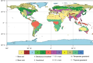
Calvet et al., 1998; Gibelin et al., 2006, 2008). The land cover is represented by nine plant functional types (PFT; given in Fig. 1) and three non-vegetated surface types that are deter-mined spatially by the ECOCLIMAP physiographic database (Masson et al., 2013a).
ISBA uses a semi-mechanistic treatment of canopy photo-synthesis and mesophyll conductance following the Jacobs et al. (1996) and Goudriaan et al. (1985) photosynthesis model. Mesophyll conductance in this framework corresponds to the rate of photosynthesis under light-saturated conditions (Ja-cobs et al., 1996). As such, this scheme does not explicitly ac-count for Michaelis–Menten kinetics of the Rubisco enzyme found in Farquhar et al. (1980) and Collatz et al. (1992) mod-els. ISBA includes a representation of the soil water stress. Key parameters of the photosynthesis model respond to the soil water stress, permitting the representation of drought-avoiding and drought-tolerant responses to drought. For low vegetation and for trees, the response to drought is based on the meta-analyses of Calvet (2000) and Calvet et al. (2004), respectively.
The model simulates a ratio of intercellular CO2 to at-mospheric CO2that depends on leaf-to-air saturation deficit, leaf temperature and soil moisture. Assimilation is calculated from this ratio, air CO2concentration, leaf temperature and solar radiation considering plant photosynthetic pathways: C3or C4(Calvet et al., 1998; Gibelin et al., 2006). Stomatal conductance, which represents the vegetation control on gas transfer (here, CO2and water vapor) between the leaves and the atmosphere, is finally deduced from the assimilation rate. Leaf dark respiration is taken as a fraction of maximum CO2 limited rate of assimilation. Standard Q10 response func-tions determine the temperature dependencies of mesophyll conductance, CO2compensation point, maximum photosyn-thetic rate and, hence, photosynthesis and respiration.
Figure 1. Fraction of dominant vegetation type as prescribed in SURFEX. This fraction results from aggregation of the various ECO-CLIMAP’s vegetation types at 1 km resolution over the T127 CNRM-ESM1 horizontal grid (∼1.4◦nominal horizontal resolution).
2002). This simple implicit nitrogen limitation is based on the nitrogen dilution hypothesis, which assumes that internal nitrogen content of a plant decrease under rising CO2due to the accumulation of non-structural carbohydrates. It results that nitrogen dilution occurs as soon as the increase in total biomass of a plant under rising CO2relative to growth under ambient CO2 is greater than the corresponding increase in total nitrogen. In current version of ISBA, a linear decrease between specific leaf area index and nitrogen to carbon ra-tio in leaves is used to mimic this mechanism (Calvet et al., 2008), and hence to limit the net assimilation of atmospheric CO2.
The soil organic matter and litter module in ISBA follows the soil carbon part of the CENTURY model (Parton et al., 1988). Four pools of litter are represented. They are differ-entiated by their location above- or belowground and their content of lignin. The litter pools are supplied by the fluxes of dead biomass from each biomass reservoir (turnover) as described in Gibelin et al. (2008). The three soil organic mat-ter reservoirs (active, slow and passive) are characmat-terized by their resistance to decomposition with turnover times span-ning from a few months for the active pool to 240 years for the passive pool. Heterotrophic respiration and hence the flux of CO2released to the atmosphere is the sum of respiration from the litter and soil organic matter reservoirs. The rate of decomposition of organic matter is determined essentially by soil moisture and temperature using a Q10 dependence
following the formulation of Krinner et al. (2005). The rate of decomposition (by respiration) depends also on the lignin fraction and the soil texture following Parton et al. (1988).
Changes in the carbon balance of the vegetation affect the energy and water balance, and hence the climate, through changes in stomatal conductance and LAI. Through its con-trol on leaf transpiration, stomatal conductance affects latent heat flux and the surface energy balance. LAI on the other hand affects evapotranspiration because it is used to scale leaf-level to canopy-level transpiration and evaporation from the interception reservoir (water intercepted by leaves).
In CNRM-ESM1, except for crops, changes in LAI do not affect the albedo of the land surface, as it is the case in some other models. As mentioned earlier, albedo is derived from satellite observations corrected in the presence of snow, but does not depend on the changes in LAI calculated by the model. This limits the biophysical feedback from vegetation change to the atmosphere.
2.3.2 Ocean biogeochemical model
nutri-ent limitation process (Aumont et al., 2003). PISCES rep-resents two size classes of phytoplankton (i.e., nanophyto-plankton and diatoms). Dependence of growth on temper-ature is parameterized according to Eppley et al. (1969). Growth rate is also limited by the external availability in nu-trients using the Michaelis–Menten relationships. Diatoms differ from nanophytoplankton by their need in silicon, by higher requirements in iron (Sunda and Huntsman, 1997) and by higher half-saturation constants because of their larger mean surface-to-volume aspect ratio. Zooplankton is repre-sented by two size classes: microzooplankton and mesozoo-plankton.
PISCES can be considered as a Monod model (Monod, 1942) since it does not represent the internal concentration of nutrients in the cells. The ratios between carbon, nitrate and phosphate are kept constant to the values proposed by Takahashi et al. (1985) in all living and non-living pools of organic matter. However, internal concentrations of iron in both phytoplankton and of silicon in diatoms are prognosti-cally simulated. They depend on the external concentration of these nutrients, on the potential limitation by the other nu-trients and on light availability.
Phytoplankton chlorophyll concentration is prognostically simulated following Geider et al. (1998). PISCES simulates semi-labile dissolved organic matter, small and big sinking particles, which differ by their sinking speeds (i.e., 3 m d−1 and 50 to 200 m d−1, respectively). Only the internal con-centrations of iron, silicon and calcite inside the sinking par-ticles are prognostically simulated. In addition to exchange with organic carbon, dissolved inorganic carbon is also al-tered by the production and dissolution of calcite. Carbon chemistry in seawater is computed from the distribution of dissolved inorganic carbon and alkalinity. Calcite is prognos-tically simulated following Maier-Reimer (1993) and Moore et al. (2002). Alkalinity includes the contribution of carbon-ate, bicarboncarbon-ate, borate and water ions. Oxygen is prognosti-cally simulated using two different oxygen-to-carbon ratios, one accounting when ammonium is converted to or mineral-ized from organic matter, the other when oxygen is consumed during nitrification. For carbon and oxygen pools, air–sea ex-change follows the Wanninkhof (1992) formulation. Impor-tantly, to ensure conservation of nitrogen in the ocean, annual total nitrogen fixation is adjusted to balance losses from den-itrification following Lipschultz et al. (1990), Middelburg et al. (1996) and Soetaert et al. (2000). For the other macronu-trients, alkalinity and organic carbon, the conservation is en-sured by tuning the sedimental loss to the total external input from rivers and dust. Therefore, carbon and nitrogen cycles are decoupled to a certain degree.
The boundary conditions account for nutrient supply from three different sources: atmospheric dust deposition for iron and silicon (Jickells and Spokes, 2001; Moore et al., 2004; Tegen and Fung, 1995), rivers for carbon (Ludwig et al., 1996) and sediment mobilization for sedimentary iron (de Baar and de Jong, 2001; Johnson et al., 1999). In
CNRM-ESM1, riverine input of carbon has been revised from Lud-wig et al. (1996) in accounting for the interannual variability of runoff estimated with an offline SURFEX simulation over the 1948–2010 period using the global atmospheric forcing from Princeton University (PGF; Sheffield et al., 2006).
In CNRM-ESM1, the marine biophysical feedback is in-duced by changes in the penetration of downward irradiance in response to marine biota chlorophyll concentration. This feedback mimics the fact that light absorption in the ocean indeed depends on particle concentration and is spectrally selective (Morel, 1988). The implementation of this mech-anism is fully described in Lengaigne et al. (2006, 2009) for an ocean forced configuration and Mignot et al. (2013) for a current ocean coupled configuration. It is derived from an accurate 61 spectral band formulation proposed by Morel (1988) using three large wavebands: blue (400– 500 nm), green (500–600 nm) and red (600–700 nm). These three bands correspond to the spectral domain of maximum absorption for chlorophyll. The chlorophyll-dependent atten-uation coefficients depend on the three-dimensional chloro-phyll field predicted by PISCES. They are computed at each time step from a power-law relationship fitting to the co-efficients computed from the full spectral model of Morel et al. (1988). This biophysical feedback represents a ma-jor evolution from the ocean component used in Voldoire et al. (2013) and Séférian et al. (2013).
3 Experimental setup 3.1 Spin-up strategy
The CMIP5 specification requires each model to reach its equilibrium state before kicking off formal simulations, es-pecially for long-term control experiments. To obtain the ini-tial conditions for CNRM-ESM1 preindustrial steady state at year 1850, we first initialize the various physical and biogeo-chemical components of the model as described below and perform a 400-year-long spin-up simulation using CNRM-ESM1 with all 1850 external forcings (Taylor et al., 2009).
Initialization of the physical components of CNRM-ESM1 relies on previous model outputs from CNRM-CM5.1. This latter model was first initialized from World Ocean Atlas 2005 observations for salinity and temperature (Antonov et al., 2006; Locarnini et al., 2006) and spun up for 200 years. The 801st year of the centennial-long CMIP5 preindustrial run from CNRM-CM5.1 was employed as initial condition for CNRM-ESM1 preindustrial state.
prein-dustrial dissolved inorganic carbon (DIC). From this initial-ization, this intermediate version of the ESM was integrated online for 1100 years.
Land biogeochemical reservoirs were initialized from zero and spun up using an acceleration approach for soil carbon and wood during the first century of the spin-up simulation. This approach consists in updating the wood growth, the lit-ter and soil biogeochemistry modules several times per time step with constant incoming carbon fluxes and physical con-ditions allowing for the various reservoirs of carbon to fill up much faster. As a result of this approach, soil carbon and wood reservoirs were respectively spun up for 21 800 and 1200 years.
Finally, both physical and carbon cycle components of CNRM-ESM1 benefit from an physical adjustment under 1850 preindustrial control conditions for 400 years. Sec-tion 4.1 describes the residual drifts of the model at quasi-equilibrium state.
3.2 CMIP5 preindustrial control and historical simulations
Following CMIP5 specifications (Taylor et al., 2009), CNRM-ESM1 has performed several CMIP5 long-term core experiments and part of the tier-1 experiments.
The preindustrial control simulation, piControl, is inte-grated for 250 years using constant external forcing pre-scribed at year 1850 conditions and starting from the last year of the online adjustment simulation. That is, atmospheric concentrations of greenhouse gases are set to 284.7 ppmv, 790.9 ppbv and 275.4 ppbv for CO2, CH4and N2O, respec-tively. Those of chlorofluorocarbons (CFC-11 and CFC-12) are set to zero. Influence of natural aerosols is prescribed us-ing the optical depths of five types of tropospheric aerosols (black carbon, sea salt, sulfate, dust and particle organic matter) from a previous simulation of the coupled Climate-Chemistry Model (LMDZ-INCA) forced with CMIP5 pre-scribed emissions (Szopa et al., 2013). Stratospheric volcanic aerosols are prescribed similarly but using a long-term av-erage climatology from a last millennium simulation per-formed with the NCAR Community Climate System Model (Ammann et al., 2007).
The 20th century experiment, historical, is performed from 1850 to 2005. This simulation starts from the CNRM-ESM1 states of the last year of the online adjustment simu-lation. The modern evolution of the external forcings of both atmospheric greenhouse gases and incoming solar irradiance follows the recommended yearly average observations (Tay-lor et al., 2009). The monthly temporal and spatial variabil-ity of the five tropospheric aerosols also rely on a LMDZ-INCA simulation (Szopa et al., 2013) while those of strato-spheric sulfate aerosol concentrations from explosive volca-noes are derived from a 20th century reconstruction of the NCAR Community Climate System Model (Ammann et al., 2007).
Note there is no land-cover change related to anthro-pogenic land use in the abovementioned simulations. The fraction of vegetal cover is set to the present-day state using the in-house ECOCLIMAP database (Masson et al., 2013a). Therefore, changes in physical and biogeochemical proper-ties of the vegetation due to actual land-cover changes are excluded by design.
4 Results
4.1 Model equilibrium in the preindustrial control simulation
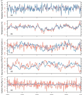
To illustrate the stability of CNRM-ESM1 at the end of the spin-up simulation, we show the global average values of a few variables during the 250 years of the piControl simula-tion (Fig. 2) and their drifts (Table 1).
In terms of energy balance, the global mean top-of-atmosphere (TOA) net radiative balance is about 3.57±0.23 W m−2, while the global mean net surface ra-diation flux (NSF) is 0.87±0.24 W m−2 (Fig. 2a). The imbalance in the energy budget between the surface and TOA (about 2.7 W m−2) is predominantly due to the non-conservation of energy of the spectral atmospheric model and, to a lesser extent, its coupling with the ocean model. Taking apart this non-conservation offset in TOA net radi-ation flux, there is no discernible deviradi-ation between year-to-year fluctuation between the TOA and NSF net radiation fluxes.
In terms of global-scale climate indices, the global mean surface temperature (T2 m)and sea surface tempera-ture (SST) over the piControl period are 12.52±0.15 and 17.76±0.1◦C, respectively (Fig. 2b). They both display al-most no drift over the duration of the piControl simulation (Table 1). We use soil wetness index (SWI) and sea sur-face salinity (SSS) to evaluate the stability of the simulated water cycle (Fig. 2c). These both have almost no drift (Ta-ble 1), confirming that the water cycle is closed. Also, there is no drift in both Northern Hemisphere and Southern Hemi-sphere sea-ice volume (NIV and SIV, respectively) for which long-term means are respectively 20.88 and 6.25×10³km3 (Fig. 2d).
R a d ia ti ve F lu xe s [W m − 2] 2 .8 3 .2 3 .6 4 −0 .2 0 .2 0 .8 1 .2 (a) T e mp e ra tu re [ °C ] 1 2 1 2 .4 1 2 .8 1 7 1 7 .4 1 7 .8 (b) H yd ro lo g ica l C ycl e [ − ] 0 .5 2 0 .5 4 0 .5 6 3 4 .5 2 3 4 .5 4 3 4 .5 6 (c) Se a I ce V o lu me [ 1 0 3km 3] 1 7 1 9 2 1 2 3 2 5 3 5 7 9 1 1 (d) Time [year] C a rb o n F lu x [P g C y − 1]
1850 1900 1950 2000 2050 2100
−0 .5 0 .5 1 .5 2 .5 −2 .5 − 1 0 1 (e)
Figure 2. Time series of various climate indices along the 250-year-long control simulation. (a) Net radiative fluxes at the top of the atmosphere (in red, leftyaxis) and surface (in blue, rightyaxis) are used to assess the stability of the climate energy flow in the model;
(b) near-surface global average temperature (in red, leftyaxis) and global-averaged sea surface temperature (in blue, rightyaxis); (c) soil
wetness index (in red, leftyaxis) and sea surface salinity (in blue, rightyaxis) are used as proxy of the hydrological cycle; (d) sea-ice volume in the Northern Hemisphere (in red, leftyaxis) and in the Southern Hemisphere (in blue, rightyaxis) are used to evaluate the stability of the cryosphere component in CNRM-ESM1; (e) global carbon fluxes over land (in red, leftyaxis) and over ocean (in blue, rightyaxis) are used to assess the equilibration of the global carbon stock. For carbon fluxes, positive (negative) fluxes indicate an uptake (outgassing) of CO2by land or ocean.
outgassing falls within the upper range of ocean inverse esti-mates (Jacobson et al., 2007; Mikaloff Fletcher et al., 2007).
4.2 Late 20th century climatology 4.2.1 Land physical drivers
In the following, we focus on the physical drivers of the global carbon cycle. From a land perspective, surface temper-ature (T2 m), precipitation (PR) and photosynthetically active radiation (PAR) are the prominent factors controlling the rate of photosynthetic activity as well as the rate of autotrophic
and heterotrophic respiration, and hence the net land–air ex-change of carbon.
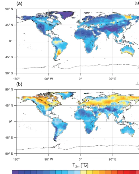
Compared to the CRUTV4 data set (Harris et al., 2013) over the period 1986–2005, CNRM-ESM1 displays a global annual-averaged bias of−3◦C in T
Fig-T able 1. Drift in climate indices used to ev aluate the equilibrium of CNRM-ESM1’ s ph ysical and biogeochemical components. The drifts are computed o v er the 250-year -long preindustrial simulation of CNRM -ESM1 for the top of the atmosphere net radiati v e balance (T O A), the net surf ace heat flux (NSF), the near -surf ace temperature ( T2 m ) , the sea surf ace temperature (SST), the sea surf ace salinity (SSS), the soil wetness inde x (SWI), the northern and southern sea-ice v olume (NIV and SIV , respecti v ely) as well as the land and ocean global carbon flux es (LCF and OCF). T O A NSF T2 m SST SWI SSS NIV SIV LCF OCF [W m − 2] [W m − 2] [ ◦C] [ ◦C] [–] [psu] [10 3km 3] [10 3km 3] [Pg C year − 1] [Pg C year − 1] Drift [units century − 1] 4.4 × 10 − 4 4.5 × 10 − 4 − 1 . 2 × 10 − 5 9.6 × 10 − 5 − 1 . 6 × 10 − 5 − 1 . 9 × 10 − 5 − 4 . 4 × 10 − 3 7 . 2 × 10 − 3 − 1 . 5 × 10 − 4 − 2 . 0 × 10 − 4
Figure 3. Biases in simulated near-surface temperature (T2 m)
com-pared to the CRUTV4 observations (Harris et al., 2013) averaged 1986–2005. Winter (a) and summer (b) periods are computed from DJFM and JJAS months.
ure 3b shows that simulated summer (i.e., JJAS: June–July– August–September) T2 m is also generally colder than the observations (−0.8◦C in global average) over a large frac-tion of the continents. Only the most northern domains of the Northern Hemisphere display a warm bias that can reach up to 3◦C in the north of Canada. The geographical struc-ture of theT2 m bias compares well with those detailed in Voldoire et al. (2013). Such an agreement in the bias struc-ture forT2 mwas expected since both models rely on the same physical parameterizations for both the atmosphere and land-surface physics. Small deviations between CNRM-CM5 and CNRM-ESM1 mean state can be essentially attributed to the land carbon cycle, which appears to amplify the global aver-age annual cold bias of 0.8◦C (with seasonal differences
be-tween CNRM-ESM1 and CNRM-CM5 of−0.7 and−1◦C
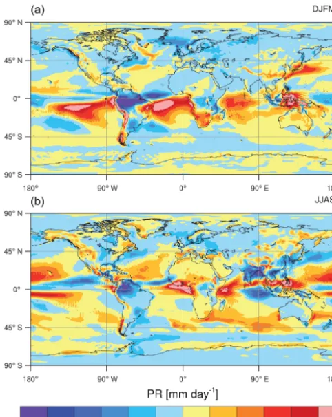
Figure 4. Biases in simulated precipitation (PR) compared to the GPCP observations (Adler et al., 2003) averaged over 1986–2005. Winter (a) and summer (b) periods are computed from DJFM and JJAS months.
coast of America and Australia. The major regional bias in seasonal PR is found over Amazonia, where PR is underesti-mated by 2 and 5 mm day−1in boreal summer and winter, respectively. Similar to state-of-the-art Earth system mod-els, CNRM-ESM1 displays an excess of precipitation over the oceans. This excess is especially strong in the southern part of the tropical oceans and is associated with the overesti-mated seasonal latitudinal migration of the Intertropical Con-vergence Zone (ITCZ). The land biosphere biophysical cou-pling induces small but noticeable changes in the global hy-drological cycle between CNRM-CM5 and CNRM-ESM1. Although weak, changes induced by the ISBA biophysical coupling slightly affect the representation of the seasonal cy-cle in PR over the vegetated regions (Fig. S1 in the Supple-ment). These lead to improve the simulated PR in CNRM-ESM1 compared to CNRM-CM5 over some vegetated re-gions during the growing season (spring–summer). Between 30 and 60◦N, the average error in simulated PR compared to GPCP is reduced by 0.12 mm day−1with CNRM-ESM1 compared to that of CNRM-CM5. Over the tropics (30◦S– 30◦N), simulated PR is also improved in CNRM-ESM1 but to a lesser extent with a reduction of the average error by 0.06 mm day−1 with respect to GPCP. Although PR have
Figure 5. Biases in simulated photosynthetically available radi-ation (PAR) compared to the Surface Radiradi-ation Budget (SRB) satellite-derived observations (Pinker and Laszlo, 1992) averaged over 1986–2005. Winter (a) and summer (b) periods are computed from DJFM and JJAS months.
been improved over some regions, their geographical pattern has been degraded in ESM1 compared to CNRM-CM5, especially during the winter.
Compared to Surface Radiation Budget (SRB) satellite-derived observations (Pinker and Laszlo, 1992), CNRM-ESM1 overestimates the PAR globally (Fig. 5). Major biases are found over continents except for some regions in the trop-ics. The magnitude of the seasonal biases is weaker in North-ern Hemisphere winter than in summer when regional biases reach up to 20–30 W m−2over the western border of the con-tinents. Regions where PAR is underestimated match reason-ably well with those showing too intense precipitations com-pared to the GPCP data set (Fig. 4). The general overestima-tion in PAR is due to the substantial underestimaoverestima-tion in low cloud cover in CNRM-ESM1 consistent with CNRM-CM5. Biases in PAR are also found over ocean upwelling system and are linked with an underestimated fraction of stratocu-mulus.
4.2.2 Ocean physical drivers
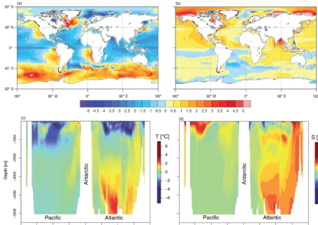
Figure 6. Annual bias patterns of simulated temperatureT and salinitySaveraged over 1986–2005 compared to the WOA2013 observations (Levitus et al., 2013). Surface biases for sea surface temperature (a) and salinity (b) are represented using the same color bar. Vertical structure of biases for temperature (c) and salinity (d) are estimated using zonal-average biases from WOA2013 across the Atlantic and Pacific oceans.
rate, playing a large role in the biological-mediated processes (e.g., export, soft tissue pump). In addition, both temperature (T) and salinity (S) control the solubility of CO2into sea-water and the chemical-mediated air–sea exchanges of car-bon. The mixed-layer depth (MLD) and the sea-ice cover (SIC) are also critical drivers of the ocean carbon cycle as they both contribute to the nutrient-to-light limitation in the high-latitude oceans (Sarmiento and Gruber, 2006). In the following, we assess the representation of these drivers.
Compared to WOA2013 data products (Levitus et al., 2013), CNRM-ESM1 realistically simulates both the mean annual sea surface temperature and sea surface salinity, both in terms of amplitude and spatial distribution, as shown in Fig. 6a and b. Moderate positive biases in sea surface temper-ature and sea surface salinity are found in the Southern Ocean and in the eastern boundary upwelling systems. Strong biases in sea surface salinity are found in the Labrador and Arctic seas. While most of these biases are related to an overesti-mated atmospheric surface heating, biases in the Labrador Sea and in the Arctic are essentially due to erroneous
rep-resentation of the mixed-layer depth and the Arctic sea-ice cover. These points will be further detailed below.
At depth, the vertical structures in simulatedT andS dis-play biases from those estimated from WOA2013 observa-tions.T is underestimated by∼2◦C within the first 1000 m
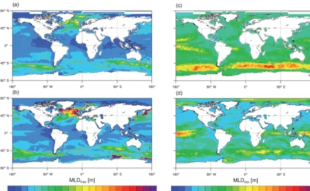
bot-Figure 7. Composite of yearly extremum of mixed-layer depth over 1986–2005. Left panels represent the maximum mixed-layer depth (MLDmax)for (a) observations (Sallée et al., 2010) and (b) CNRM-ESM1. Right panels represent the minimum mixed-layer depth (MLDmin)
for observations (c) and CNRM-ESM1 (d).
tom water (AABW) is about 11.6±1 Sv in CNRM-ESM1 averaged over the 1850–2005 period. This flow of AABW is in agreement with the deep flow of waters compared to the observed estimate of 10±2 Sv (Orsi et al., 1999). Conse-quently, the flow of deep water masses in CNRM-ESM1 has been improved with regards to that of CNRM-CM5, which ranges between 3.4 and 6.2 Sv over the same period (Séférian et al., 2013; Voldoire et al., 2013). As detailed in several in-tercomparison studies (de Lavergne et al., 2014; Heuzé et al., 2013; Sallée et al., 2013; Séférian et al., 2013), CNRM-CM5 substantially underestimated the flow of AABW lead-ing to an erroneous distribution of hydrodynamical and bio-geochemical fields at depth. Here, although stronger than the observation-based estimates, the flow of NADW and AABW improves the deep ocean ventilation as well as the distribu-tion of tracers at depth (Sect. 4.2.5).
As mentioned above, an accurate representation of spa-tial and temporal MLD is essenspa-tial for numerous ocean biogeochemical processes. For example, winter mixing en-trains carbon- and nutrient-rich deep waters to the surface, which play an important role in the transfer of CO2 across the sea-to-air interface. In summer, MLD contributes to the nutrient-to-light limitation of the phytoplankton growth in high-latitude oceans. The maximum and minimum mixed-layer depth (hereafter, MLDmax and MLDmin)are respec-tively used as a proxy of the winter and summer MLD since
mixing occurs randomly during seasons in response to nu-merous environmental factors (wind, stratification, local in-stability, etc.) that present a large spatiotemporal variabil-ity. Figure 7 presents composites of yearly MLDmax and MLDminas simulated by CNRM-ESM1 in averaged over the 1986–2005 period and derived from observations (Sallée et al., 2010). Figure 7a and b show that CNRM-ESM1 repro-duces the main regional pattern of MLDmaxcompared to the observation-derived estimates. However, the model tends to simulate too large and too deep mixing sites in the North Atlantic, the North Pacific and the Southern Ocean. In the North Atlantic, the larger than observed mixed volume of surface dense waters (combination of surface area and depth of the mixing zone) is at the origin of the strong flow of NADW simulated in CNRM-ESM1. In the Southern Ocean, although open-ocean polynyas were observed from space in the past decades (Cavalieri et al., 1996; Comiso, 1999), their locations are erroneous in CNRM-ESM1 similarly to several other CMIP5 Earth system models (de Lavergne et al., 2014). CNRM-ESM1 simulates open-ocean polynyas in the Indian basin and close to the Ross Sea but not in the Atlantic basin as observed from space between 1974 and 1976.
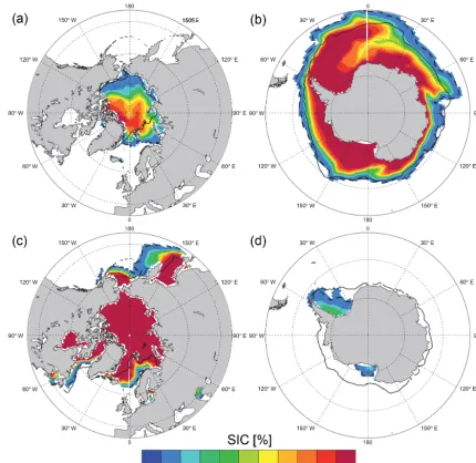
Figure 8. Sea-ice cover (SIC) as simulated by CNRM-ESM1 averaged over 1986–2005. Top panels represent composite of September sea-ice cover, while bottom panels are for March. Iso-15 % of SIC serves as comparison between model results and NSIDC observations (Cavalieri et al., 1996) averaged over 1986–2005; model results and observations are indicated with dashed and solid black lines, respectively.
the current parameterization of the ocean mixing employed in CNRM-ESM1 because previous model versions using this parameterization also exhibited similar patterns of errors as detailed in Séférian et al. (2013) and Voldoire et al. (2013).
Similarly to the MLD, SIC is an important driver of the ocean carbon cycle. It constitutes a physical barrier for ex-change of CO2between the ocean and the atmosphere lead-ing to an accumulation of carbon-rich waters below the sea ice (Takahashi, 2009). It also plays a large role in the seasonal timing of algal blooms (Wassmann et al., 2010). Compared to the MLD, seasonal variations of sea ice are strongly and di-rectly responsive to the seasonal fluctuations of atmospheric forcing. Therefore, it matters that the model is able to accu-rately capture the spatial distribution and timing of annual
Centered SD (σ)
Ce
nt
er
ed
SD (
σ
)
0.0 0.5 1.0 1.5
0.0
0.5
1.0
1.5
0.5 1 1.5
0.1 0.2 0.3 0.4 0.5
0.6 0.7
0.8
0.9 0.95
0.99 Corre
lation
Correlation (a) Land surface
T2m
PR PAR
(b) Ocean SST SSS MLD PR
0.0 0.5 1.0 1.5
0.0
0.5
1.0
1.5
0.5 1 1.5
0.1 0.2 0.3 0.4
0.5 0.6
0.7 0.8
0.9 0.95
0.99
Centered SD (σ)
Figure 9. Taylor diagrams showing the correspondence between model results and observations for CNRM-ESM1 and CNRM-CM5.2. Near-surface temperature (T2 m), precipitation (PR) and photosynthetically available radiation (PAR) are used to assess model performance
over land surface. Sea surface temperature (SST), sea surface salinity (SSS), mixed-layer depth (MLD) and precipitation (PR) are used to assess model performance over ocean. Filled and empty symbols indicate skills for CNRM-ESM1 and CNRM-CM5.2, respectively. The size of the symbols indicates whether statistics were computed from annual mean climatology or seasonal average (JFM, AMJ, JAS, OND) over 1986–2005.
along with positive SST biases in this region (Fig. 6a), and explains why the simulated deep convection zone is too large and shifted northward in CNRM-ESM1 as shown in Fig. 7.
In the Antarctic Ocean, Fig. 8b shows that the spatial structures of SIC biases mirror somehow the model–data mismatch in MLD as shown in Fig. 7b. That is, in austral winter, CNRM-ESM1 underestimates SIC where erroneous open-ocean deep convection zones are located, namely, off-shore Wilkes Land in the Indian Ocean sector (Fig. 8b). Con-versely, too much sea ice is simulated in the Atlantic Ocean sector. As in CNRM-CM5.1, simulated summer Antarctic SIC is strongly underestimated, with very little sea ice sur-viving summer melt in the Weddell and Ross seas (Fig. 8d).
4.2.3 Comparison with previous model version
In the following, we compare the skill of CNRM-ESM1 to the closest version of CNRM-CM5 climate model, called CNRM-CM5.2. Figure 9 summarizes skill-assessment met-rics for CNRM-ESM1 and CNRM-CM5.2 in terms of major physical drivers of the global carbon cycle (field maps and patterns of errors are presented in Figs. S2 to S7).
The Taylor diagram for land-surface physical drivers clearly demonstrates that CNRM-ESM1 and CNRM-CM5 display comparable skills except for PR (Fig. 9a). Most of the differences in skills are indeed not significant at a 95 % con-fidence level; models differ solely in terms of PR for which CNRM-ESM1 produces slightly weaker correlation coeffi-cients.
Over the ocean, Fig. 9b shows further differences be-tween both models. The weakest difference in skill concerns SST for which both models display good agreement with
WOA2013. With regard to the MLD, CNRM-ESM1 dis-plays a slightly better agreement than CNRM-CM5.2 with observation-derived MLD (Sallée et al., 2010) in terms of correlation but strongly underestimates the spatial varia-tions of this field. Major differences are noticeable for SSS. ESM1’s skill is clearly lower than that of CNRM-CM5.2. To investigate this difference, we have computed the skill of PR over the ocean, since CNRM-CM5.2 contributes to the spatiotemporal distribution of the SSS concomitantly to the runoff and the sea-ice seasonal cycle. Skill in PR over the ocean is similar for both models (blue diamonds on Fig. 9b). A similar finding is noticed for simulated runoff (not shown). Therefore, the difference in simulated SSS be-tween the two models can be attributed to the revised water conservation interface and erroneous distribution of sea-ice cover. In addition, changes in coupling frequency (i.e., 24 to 6 h) might be at the origin of differences in skills between the two models since it impacts sea-ice cover (Fig. 10).
From the small differences in skill between the two mod-els, we can assume that the inclusion of the global carbon cy-cle and the biophysical coupling have not noticeably altered the simulated mean-state climate in CNRM-ESM1 compared to that of CNRM-CM5.2.
4.2.4 Terrestrial carbon cycle
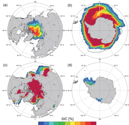
Figure 10. Impact of coupling frequency on sea-ice cover (SIC) as simulated by CNRM-ESM1 averaged over 1986–2005. Top panels represent composite of September sea-ice cover, while bottom panels are for March. Iso-15 % of SIC serves as comparison between model results using a 6 h coupling frequency (dashed lines) and those using a 24 h coupling frequency (solid lines).
CO2 on land. Simulated budget of vegetation biomass and total ecosystem respiration (TER; sum of autotrophic and heterotrophic respirations) are evaluated against available published estimates. While we can assess the capability of CNRM-ESM1 to fix and emit carbon on land, it is important to note that the CO2fluxes due to land use changes are not taken into account in this analysis.
To evaluate CNRM-ESM1 GPP, we rely on two streams of data, namely, the FluxNet-Multi-Tree Ensemble (FluxNet-MTE, Jung et al., 2011) and the MOD17 satellite-derived ob-servations (Running et al., 2004). Figure 11 shows that the annual mean GPP as simulated by CNRM-ESM1 is slightly too strong compared to the observed estimates. The largest model–data mismatch is found in the tropics between 10◦N
Figure 11. Annual-mean terrestrial gross primary production (GPP). Values are given for (a) observation-derived FluxNet-MTE (Jung et al., 2011) averaged over 1986–2005, (b) satellite-derived observation from MODIS over 2000–2013 and (c) CNRM-ESM1 over 1986–2005.
60 Pg C year−1. Regional biases in GPP are partly compen-sated by overestimated Ra (Fig. 12). Simulated Ra agrees reasonably well with satellite-derived estimates except in the tropics. This bias compensation between GPP and Ra is an-alyzed in detail by Joetzjer et al. (2015). In this study, the authors demonstrate that the current parameterizations of Ra and water stress in ISBA are not adequate for tropical broadleaf trees (Fig. 1). Considering that these results were
deduced from offline simulations forced with in situ observa-tions, we can assume here that biases in GPP and Ra result from a combination of erroneous ecophysiological parame-terizations and biases in physical drivers in CNRM-ESM1.
Table 2. Regional and global budget of gross primary production (GPP) and terrestrial ecosystem respiration (TER) as simulated by the CNRM-ESM1 and estimated from the FluxNet-MTE data product. Values in brackets indicate the ratio between the autotrophic respiration (Ra) and TER. The uncertainties for the FluxNet-MTE data product derive from the regional partitioning of global mean uncertainties published in Jung et al. (2011). GPP and TER fluxes are determined from a yearly average over 1986–2005.
Regions CNRM-ESM1 MTE-FluxNet CNRM-ESM1 MTE-FluxNet
GPP [Pg C year−1] TER [Pg C year−1]
High-latitude north (>60◦N) 2.6 4.8±0.8 2.5 (38 %) 3.1±0.8
Mid-latitude north (20–60◦N) 37.9 34.8±2.7 36.23 (52 %) 29.9±2.7
Tropics (20◦S–20◦N) 73.2 62.3±1.9 72.58 (72 %) 54.8±1.9
Mid-latitude south (20–60◦S) 16.1 9.3±0.6 15.6 (56 %) 8.5±0.6
Global 130.0 111.3±6.0 126.9 (64 %) 96.4±6.0
Figure 12. Annual-mean autotrophic respiration (Ra) as estimated from MODIS over 2000–2013 (a) and as simulated by CNRM-ESM1 (b) over 1986–2005. Panel (c) represents the zonal-cumulated Ra in function of latitude for both satellite-derived estimates (in blue) and CNRM-ESM1 (in red).
2007), respectively. Furthermore, the geographical structure of cSoil agrees well with Harmonized World Soil Database (JRC, 2012) except in the Northern Hemisphere (Fig. 13). Although several processes are missing in ISBA to accurately simulate high-latitude carbon stock (e.g., permafrost dynam-ics, bacterial degradation of the litter, fire-induced turnover), a part of cSoil underestimation can be attributed to the sum-mer warm bias in near-surface temperature (Fig. 3b). This latter tends to enhance heterotrophic respiration of the soil, reducing the soil organic matter (R >0.6, Fig. S2).
Table 2 shows that CNRM-ESM1 overestimates globally terrestrial ecosystem respiration (TER) when compared to the up-scaled measurements of FluxNet-MTE. In the tropics, simulated TER fluxes are 32 % higher than the FluxNet-MTE estimates. As mentioned above, this bias is essentially due to an unrealistic Ra, which amounts to 72 % of TER over the sector in the model. Table 2 shows that the simulated TER is 126.9 Pg C year−1, larger than estimates published by Jung et al. (2011) of 96.4±6.0 Pg C year−1. Nevertheless, the simu-lated net land carbon sink (LCS), which can be estimated by subtracting TER from GPP, is 2.19 Pg C year−1in aver-age over the 1986–2005 period and remains within the range
of values estimated from various observation-based methods (IPCC, 2007, 2013; Le Quéré et al., 2014).
4.2.5 Ocean carbon cycle
Figure 13. Stocks of modern soil organic carbon (cSoil) as estimated from the FAO/IIASA/ISRIC/ISSCAS/JRC (2012) Harmonized World Soil Database (a) and as simulated by CNRM-ESM1 (b) averaged over 1986–2005. Panel (c) represents the zonally cumulated soil organic stock in function of latitude for both observation-based estimates (in blue) and CNRM-ESM1 (in red).
Tracers: O2 PO4 NO3
SiO2
Depth levels: Surface 150 m 1000 m 2500 m 5000 m
Centered SD (σ)
Ce
nt
er
ed
SD (
σ
)
0.0 0.5 1.0 1.5
0.0
0.5
1.0
1.5
0.5 1 1.5
0.1 0.2 0.3 0.4
0.5 0.6
0.7 0.8
0.9 0.95
0.99 Correlation
0.0 0.5 1.0 1.5
0.0
0.5
1.0
1.5
0.5 1 1.5
0.1 0.2 0.3 0.4
0.5 0.6
0.7 0.8
0.9 0.95
0.99 Correlation
0.0 0.5 1.0 1.5
0.0
0.5
1.0
1.5
0.5 1 1.5
0.1 0.2 0.3 0.4
0.5 0.6
0.7 0.8
0.9 0.95
0.99 Correlation
0.0 0.5 1.0 1.5
0.0
0.5
1.0
1.5
0.5 1 1.5
0.1 0.2 0.3 0.4
0.5 0.6
0.7 0.8
0.9 0.95
0.99 Correlation
Ce
nt
er
ed
SD (
σ
)
Ce
nt
er
ed
SD (
σ
)
Ce
nt
er
ed
SD (
σ
)
Centered SD (σ)
Centered SD (σ) Centered SD (σ)
Figure 14. Taylor diagrams showing the correspondence between model results and observations for CNRM-ESM1 and CNRM-CM5.2 (Séférian et al., 2013). Climatological distribution over 1986–2005 of simulated oxygen (O2), phosphate (PO4), nitrate (NO3)and silicate
(SiO2)concentrations are assessed against WOA2013 data product. Filled and empty symbols indicate skills for ESM1 and CNRM-CM5, respectively. The size of the symbols indicates the depth at which statistics have been computed.
distribution (R∼0.4). In addition to nutrients, the vertical distribution of carbon-related fields like dissolved inorganic carbon has been substantially improved in CNRM-ESM1 compared to CNRM-CM5 (Fig. S9), showing a much
bet-ter agreement with Global Data Analysis Project (GLODAP) observations (Key et al., 2004; Sabine et al., 2004).
Figure 15. Annual-mean ocean carbon fluxes (fgCO2)as estimated by the Takahashi et al. (2010) database (a) and as simulated by
CNRM-ESM1 averaged over 1986–2005 (b). Panel (c) represents the zonal-cumulated carbon fluxes in function of latitude for both observation-based estimates (in blue) and CNRM-ESM1 (in red). Negative (positive) fluxes indicate an uptake (outgassing) of CO2.
to 2005 together with observation-based estimates by Taka-hashi et al. (2010) using 2000 as a single reference year. While the model broadly agrees with the observations in terms of spatial variation for regions of carbon sink (i.e., North Atlantic, North Pacific and between 50 and 40◦S), it displays a too strong source of carbon to the atmosphere in the equatorial Pacific and in the Southern Ocean. In the equatorial Pacific, the model–data mismatch is likely related to the decision of Takahashi et al. (2010) to exclude obser-vations from El Niño years from their analysis. Since sur-face ocean pCO2 of the eastern tropical Pacific during El Niño events tends to be lower than the long-term mean, the Lamont–Doherty Earth Observatory (LDEO) climatol-ogy tends to underestimate outgassing of CO2 in the equa-torial Pacific over the 1986–2005 period. This hypothesis is validated when comparing model results against recent data products derived from statistical Monte Carlo Markov chain or neural network gap-filling methods (Landschützer et al., 2014; Majkut et al., 2014, Fig. S10). In the Southern Ocean, the model–data mismatch is especially pronounced south of 60◦S. This bias in fgCO2 is associated with overestimated mixing (Fig. 7), which tends to bring too much deep carbon-rich water masses to the surface, enhancing the outgassing of CO2. CNRM-ESM1 results display similar discrepan-cies when compared to other recent observation-derived data products, which coincide with regard to a moderate CO2 out-gassing south of 60◦S (Fig. S10). That said, simulated pat-terns of sea-to-air carbon fluxes in this domain qualitatively agree with the data, showing a combination of source and sink regions.
The storage of anthropogenic CO2 by the oceans (COANTH2 , Fig. 16) provides a complementary view of the ocean carbon fluxes by revealing the chronology of the ocean CO2 uptake from preindustrial to modern state. Here, we
Figure 16. Annual-mean zonal-average anthropogenic carbon (COANTH2 )across the Atlantic and Pacific oceans as simulated by CNRM-ESM1 averaged over 1990–2005 (a) and as estimated from the GLODAP database compiling data up to 1994 (b). Panel (c) represents the mean-annual bias in zonal structures between model and observation-based estimates in COANTH2 .
4.2.6 Ecosystem dynamics
In this section, we assess the performance of CNRM-ESM1 in terms of two ecosystem dynamics parameters, namely, the peak leaf area index (LAImax)and the ocean surface chloro-phyll (Chl). Both parameters have been monitored continu-ously from space since the 1980s and the 1990s, respectively, providing a suitable set of indirect observations to assess the simplified ecosystem representation embedded in Earth sys-tem models.
With regard to LAImax, Fig. 17 shows that the model agrees well with satellite-derived observations (Zhu et al., 2013) except over Africa and Asia with overestimated val-ues. As such, this ecosystem parameter behaves similarly to GPP and Ra, responding to biases in PR and PAR. In the northern mid-latitudes, LAImaxis slightly overestimated compared to the satellite-derived observations but remains in the low range of values simulated by other CMIP5 Earth sys-tem models evaluated in Anav et al. (2013b). Using an offline
Figure 17. Composite of yearly maximum of leaf area index (LAImax)as estimated from AVHRR satellite observations of Zhu et al. (2013)
(a) and as simulated by CNRM-ESM1 (b) over 1986–2005. Panel (c) represents the zonal-average LAImaxin function of latitude for both
observation-based estimates (in blue) and CNRM-ESM1 (in red).
Figure 18. Annual-mean surface chlorophyll concentrations (Chl) as estimated from SeaWiFS over 1997–2010 (a) and as simulated by CNRM-ESM1 (b) over 1986–2005. Panel (c) represents the zonal-averaged Chl in function of latitude for both satellite-derived estimates (in blue) and CNRM-ESM1 (in red).
partly explains why Chl concentrations are underestimated in high-latitude oceans. In these domains, high coastal con-centrations are captured from satellite sensors but cannot be resolved by the model due to its coarse resolution.
4.3 Recent evolution of the climate system
In the present section, we analyze the transient response of various climate indices to the recent climate forcing from 1901 to 2005. We focus on the near-surface temperature (T2 m), the September Arctic sea-ice extent (SIE), the 0– 2000 m ocean heat content (OHC) as well as the land and ocean carbon sinks (LCS and OCS, respectively). Over this period, these climate indices are analyzed with their nom-inal values except for T2 m and OHC that are represented with respect to the 1961–1990 and the 1955–2005 periods, respectively. Figure 19 illustrates how these various climate indices evolve from 1901 to 2005 and Table 3 summarizes
their mean-state, interannual variability (IAV) and decadal trends over the 1986–2005 period.
T e mp e ra tu re [ °C ] −1 .5 − 1 −0 .5 0 0 .5 (a) A rc ti c s e a i c e e x te n t [ 1 0 k m ] 6 2 O c e a n he a t co n te n t [ 1 0 J ] 2 2 L a n d ca rb o n fl u x [ P g C y − 1] −2 0 1 2 3 4 5 6 (d) O c e a n ca rb o n fl u x [ P g C y ] − 1 −1 0 1 2 3 (e) Time [year]
1900 1920 1940 1960 1980 2000
2 3 4 5 6 7 8 9 (b) −1 0 −5 0 5 1 0 1 5 (c)
Figure 19. Time series of various climate indices as monitored from available observations (blue solid line) and as simulated by CNRM-ESM1 (red solid line) since 1901 with global near-surface temperature (a), September Arctic sea-ice extent (b), 0–2000 m ocean heat content
(c), land carbon flux (d) and ocean carbon flux (e). Hatching represents the±2σ estimated from the ensemble deviation between the 100
members of the HadCRUT4 database (Morice et al., 2012) for near-surface temperature, the standard deviation between two National Snow and Ice Data Center estimates (Fetterer et al., 2002; Comiso, 1999) and Hadisst (Rayner et al., 2003) databases, the pentadal variability of the observed ocean heat content (Levitus et al., 2012) and spread between Global Carbon Project reconstructions for both land and ocean (Le Quéré et al., 2014). For both OCS and LCS, positive (negative) fluxes indicate an uptake (outgassing) of CO2.
also the decadal decrease in extent (Table 3). Therefore, in terms of Arctic sea ice, the skill of CNRM-ESM1 is simi-lar to CNRM-CM5 as detailed in Massonnet et al. (2012). A better agreement is found for OHC for which CNRM-ESM1 results agree with observation-based estimates in term of mean-state and decadal trends (Fig. 19, Table 3). Only the recent IAV in OHC is underestimated by the model, but the
latter is poorly constrained by the observations with regard to the small amount of data available below 1000 m (Levitus et al., 2012, 2009; Willis et al., 2004).
Table 3. Modern mean-state, interannual variability (IAV) and decadal trends of various global climate indices: the near-surface temperature (T2 m), Arctic September sea-ice extent (SIE), 0–2000 m ocean heat content (OHC) as well as the land and ocean carbon sinks (LCS and
OCS, respectively). For LCS and OCS, positive values indicate an uptake of CO2by land and ocean. All metrics are computed over the
1986–2005 period for both model and observations. Decadal trends are estimated from linear regression over the 1986–2005 period. IAV is estimated from the standard deviation of the detrended time series.
CNRM-ESM1 Observations
mean 0.43 0.30±0.08 (Morice et al., 2012)
T2 m[◦C] IAV 0.13 0.10
trend 4.0×10⁻² 2.6×10⁻²
mean 4.68 6.70±0.26 (Comiso, 1999; Fetterer et al., 2002; Rayner et al., 2003)
SIE [106km2] IAV 1.14 0.46
decadal −16×10−2 −6.8×10⁻²
mean 3.34 3.50±1.42 (Levitus et al., 2012)
OHC [1022J] IAV 0.69 1.43
trend 0.44 0.50
mean 2.19 2.06±1.0 [models] (Le Quéré et al., 2014)
2.19±0.8 [residual land carbon sink] (Friedlingstein et al., 2010)
LCS [Pg C year−1] IAV 0.59 1.01
trend 0.3×10⁻² 1.8×10⁻²
mean 1.65 1.87±0.4 [models] (Le Quéré et al., 2014) 2.15±0.5 [obs.-models combination] 2.0±0.7 (Takahashi et al., 2010)
OCS [Pg C year−1] IAV 0.09 0.14
trend 4.5×10⁻² 1.8×10⁻²
respectively (Table 3). Underestimation in mean-state OCS is essentially due to the stronger river-induced offshore out-gassing of CO2, which is about 0.9 Pg C year−1in the model and assumed to be of 0.45 Pg C year−1 in the observation-derived estimates. Both OCS and LCS IAV are underesti-mated in CNRM-ESM1 compared to the estimates. For OCS IAV, this behavior is found in most ocean biogeochemical models as shown in Wanninkhof et al. (2013). Indeed, sim-ulated IAV from biogeochemical models substantially con-trasts with the large IAV estimated from atmospheric inver-sion, which also contributes to the mix of observations and model reconstructions that compose the data (Le Quéré et al., 2014). For the land carbon cycle, underestimated LCS IAV may be related to the under-sensitivity of ISBA to cli-mate variability in contrast with the over-sensitivity to the ris-ing CO2, a behavior shared with other land-surface process-based models (Piao et al., 2013). Note that differences in phase between simulated and estimated LCS were expected since the land sink of carbon is approximated from the dif-ference between atmospheric growth rate, land use emissions and ocean carbon sink (Friedlingstein et al., 2010).
5 Summary and conclusions
In this article, we evaluate the ability of the Centre National de Recherches Météorologiques Earth system model version
< 0.0 0.2 0.4 0.6 0.8 1.0 C ESM1 −BG C C MC C −C ESM C N R M−ESM1 C a n ESM2 G F D L −ESM2 G G F D L −ESM2 M G ISS−E2 −H −C C G ISS−E2 −R −C C H a d G EM2 −C C H a d G EM2 −ES IPSL −C M5 A−L R IPSL −C M5 A−MR IPSL −C M5 B−L R MI R O C −ESM−C H EM MI R O O C −ESM MPI −ESM−L R MPI −ESM−MR MR I−ESM1 N o rESM1 −ME 0.0 0.5 1.0 1.5 > 2.0 L AI G PP R a R h cSo il fg C O2 C h l O2 N O3 PO 4 Si (a) Correlation
(b) Root-mean-squared error
L AI G PP R a R h cSo il fg C O2 C h l O2 N O3 PO 4 Si
Figure 20. Skill-score matrix based on (a) spatial correlation and (b) globally averaged root mean squared error for relevant fields of the simulated carbon cycle from current generation Earth system models. Leaf area index (LAI), gross primary productivity (GPP), autotrophic respiration (Ra), heterotrophic respiration (Rh) and soil carbon (cSoil) are used to assess model skill in terms of modern mean-state terrestrial carbon cycle. Sea–air carbon flux (fgCO2), surface chlorophyll (Chl) and surface concentrations of oxygen (O2), nitrate (NO3), phosphate
(PO4)and silicon (Si) are used to evaluate the skill of the current models at replicate modern mean-state ocean carbon cycle. Both models and
observed fields are averaged over time from 1986 to 2005 to determine skill score metrics, except for cSoil, O2, NO3, PO4, Si observations
(only a modern mean-state climatology is available). Black squares indicate that models fields are not available (implying that these fields are either not simulated by the model or not published on the Earth System Grid Federation, ESGF).
soil carbon stock over the last decades. Although the pho-tosynthesis scheme in ISBA differs from the other state-of-the-art process-based models (e.g., Dalmonech et al., 2014), the model displays similar behavior. That is, it overestimates both the land–vegetation gross primary productivity and the terrestrial ecosystem respiration. The compensation between these two fluxes leads to a correct land carbon sink over the modern period that agrees with the most up-to-date estimates