Numerical simulations of oceanic oxygen cycling in the FAMOUS Earth-System model: FAMOUS-ES, version 1.0

(1)

Geosci. Model Dev., 7, 1419–1431, 2014 www.geosci-model-dev.net/7/1419/2014/ doi:10.5194/gmd-7-1419-2014

Numerical simulations of oceanic oxygen cycling in the FAMOUS

Earth-System model: FAMOUS-ES, version 1.0

J. H. T. Williams1, I. J. Totterdell2, P. R. Halloran3,*, and P. J. Valdes1

1_{BRIDGE, School of Geographical Sciences, University of Bristol, Bristol, BS8 1SS, UK} 2_{Met Office Hadley Centre, FitzRoy Road, Exeter, EX1 3PB, UK}

3_{School of Geography, University of Exeter, Exeter, EX4 4RJ, UK}

*_{previously at: Met Office Hadley Centre, FitzRoy Road, Exeter, EX1 3PB, UK} Correspondence to: J. H. T. Williams ([email protected])

Received: 9 January 2014 – Published in Geosci. Model Dev. Discuss.: 21 February 2014 Revised: 3 June 2014 – Accepted: 4 June 2014 – Published: 15 July 2014

Abstract. Addition and validation of an oxygen cycle to the ocean component of the FAMOUS climate model are described. At the surface, FAMOUS overestimates north-ern hemisphere oxygen concentrations whereas, at depth, the southern hemisphere values are too low. Surface validation is carried out with respect to HadGEM2-ES where, although good agreement is generally found, discrepancies are mainly attributed to disagreement in surface temperature structure between the models. The disagreement between the models at depth in the Southern Hemisphere is attributed to a combi-nation of excessive surface productivity in FAMOUS’ equa-torial waters (and its concomitant effect on remineralisation at depth) and its reduced overturning circulation compared to HadGEM2-ES. For the Atlantic basin FAMOUS has a cir-culation strength of 12.7±0.4 Sv compared to 15.0±0.9 for HadGEM2-ES. Global- and basin-scale decomposition of meridional overturning circulation, oxygen concentration and apparent oxygen utilisation (AOU) – a measure of the de-parture from equilibrium with the atmosphere – allows spe-cific features of the climatology to be assigned to particu-lar basins. For example, the global signal in overestimation of low-latitude Northern Hemisphere oxygen at intermediate depths is attributed to the Pacific. In addition, the inclusion of the AOU analysis enables explanation of oxygen-deficient deep water in the Southern Hemisphere which is not seen in the Northern Hemisphere.

1 Introduction

The ongoing model development of the FAMOUS climate model (Jones et al., 2005; Smith et al., 2008; Smith, 2012; Williams et al., 2013) in contrast to its higher resolution par-ent model HadCM3 (Gordon et al., 2000; Pope et al., 2000) is a testament to its utility as a fast (Fast Met Office UK Uni-versities Simulator; FAMOUS) model which is capable of running at least 10 times faster than HadCM3. Model devel-opment with the latest Met Office Hadley Centre models con-tinues apace however. Indeed huge improvements in model physics too numerous to detail here have been achieved via HadCM4 (Webb et al., 2001), HadGEM1 (e.g. Martin et al., 2006), HadGEM2 (e.g. Collins et al., 2011) and HadGEM3 (Hewitt et al., 2011), arguably the most notable of which are the introduction of a new semi-Lagrangian dynamical core in HadGEM1, and new ocean and cloud schemes in HadGEM3. It is not just the physical model components which have un-dergone model development however. HadCM3LC was the first coupled climate model to include a fully interactive car-bon cycle (Cox et al., 2000). HadGEM2-ES has extended the Earth System complexity represented within HadCM3LC by evolving the ocean carbon cycle sub-model, as well as the addition of a non-sulfate aerosols, aerosol indirect effects, interactive dust emission, and interactive tropospheric chem-istry (Collins et al., 2011; Bellouin et al., 2011).

(2)

1420 J. H. T. Williams et al.: Oceanic oxygen cycling in FAMOUS

The continued use of the HadCM3 family of models is justified since it has been shown to continue to perform well compared to more recent models. For example, Reichler and Kim (2008) show that HadCM3 performs statistically better than many other models in the Intergovernmental Panel on Climate Change’s “CMIP3” archive despite having been doc-umented several years earlier. In addition to this, FAMOUS is capable of running for sufficiently long to allow more slowly evolving components of the Earth system to be investigated. There are many potential applications of the new model functionality presented here, for example Cretaceous oceanic anoxic events, OAEs (e.g. Monteiro et al., 2012). These were episodes in which potentially the entire global ocean was sig-nificantly depleted in oxygen, clearly with huge ramifications for global biogeochemical cycles. This paper however will focus solely on the model development undertaken to include cycling of oxygen in the FAMOUS model.

Previous oxygen modelling studies include those of Matear et al. (2000) (with particular focus on future changes to the Southern Ocean), Bopp et al. (2002) (trends in ocean– atmosphere oxygen fluxes, including partitioning into ocean surface warming and changes in stratification) and Frölicher et al. (2009) (small ensemble of climate simulations studying both human- and volcanically induced perturbations to the ocean’s oxygen cycle). An excellent review of oxygen mod-elling with particular reference to hypoxic (reduced oxygen) waters can be found in Peña et al. (2010) and a detailed dis-cussion of P / N / Corg/ O2 (Redfield) ratios in seawater can be found in Anderson and Sarmiento (1994).

2 Theory and model description

This work describes the inclusion of oxygen cycling into FA-MOUS’ ocean GCM (General Circulation Model) code. The method followed is that of the second phase of the Ocean Carbon-Cycle Model Intercomparison Project, OCMIP2, as specifically implemented into the HadGEM2-ES code. The formalism used is that of Garcia and Gordon (1992) via the protocols of the Ocean Carbon-Cycle Model Intercompari-son Project (Najjar and Orr, 1999). Full details of the bio-geochemical cycling system present in FAMOUS (without oxygen) can be found in Palmer and Totterdell (2001). In the present work, the rate of biological production of oxygen is simply proportional to the rate of consumption of DIC (dis-solved inorganic carbon),

dO dt = −α

dC

dt, (1)

where O and C are the concentrations of oxygen and car-bon (represented by dissolved inorganic carcar-bon, DIC, in the model) andαis the constant of proportionality (equal to138₁₀₆). More information on the precise origin of this coefficient’s value can be found in Anderson and Sarmiento (1994). Al-though the continuity equations of oxygen and carbon diox-ide are trivially similar, the form of the air–sea flux equations

is quite different for oxygen. The form of the flux is as fol-lows:

FO=ρk (1−A) (Osat−O) . (2)

In this equation, the fluxFOis a function of the water density ρ, the fractional coverage of sea ice (in each grid box)A, the “piston velocity”k and the oxygen concentration at satura-tion point, Osat. The functional forms ofkand Osatare now given:

k=0.31u2

r 660

Sc (3)

Osat=

1000eA

22.3916, (4)

whereu is the wind speed and Sc is the Schmidt number (Keeling et al., 1998),

Sc=1638+Tc(−81.83+Tc(1.483−0.008004Tc)) , (5) andA(lnC0in Garcia and Gordon, 1992) is given by A=2.00907+3.22014Ts+4.05010Ts2+4.94457Ts3

−0.256847T_s4+3.88767T_s5+H−6.24523×10−3

−7.37614×10−3Ts+1.03410×10−2Ts

−8.17083×10−3T_s3−4.88682×10−7S2.

In these equations,TcandTsare given by

Tc=max(−2,MIN(40, T+273.15)) (6) and

Ts=ln

₅_.₇₁₃

MAX(2.71,0.01(273.15+T ))

−1

, (7)

whereT is the temperature in degrees Celsius andS is the salinity in practical salinity units (PSU). Note that Eq. (7) is from the text in Garcia and Gordon (1992) immediately following their Eq. (8), and that a minimum temperature of

−2.15◦ _{has been imposed to prevent divergence resulting} from a vanishing denominator. It should also be noted that Eq. (8) in Garcia and Gordon (1992) contains an error, which is corrected in the OCMIP protocols and therefore in our code (Najjar and Orr, 1999). Finally, the air–sea boundary condition is given by

dO dt =

FO 1z1

, (8)

where1z1is the depth of the first level in the ocean GCM vertical grid. In the preceding equations, the units are as fol-lows: Osat(Mol m−3),k (m2s−2) and Sc,A andTs are di-mensionless.

(3)

J. H. T. Williams et al.: Oceanic oxygen cycling in FAMOUS 1421

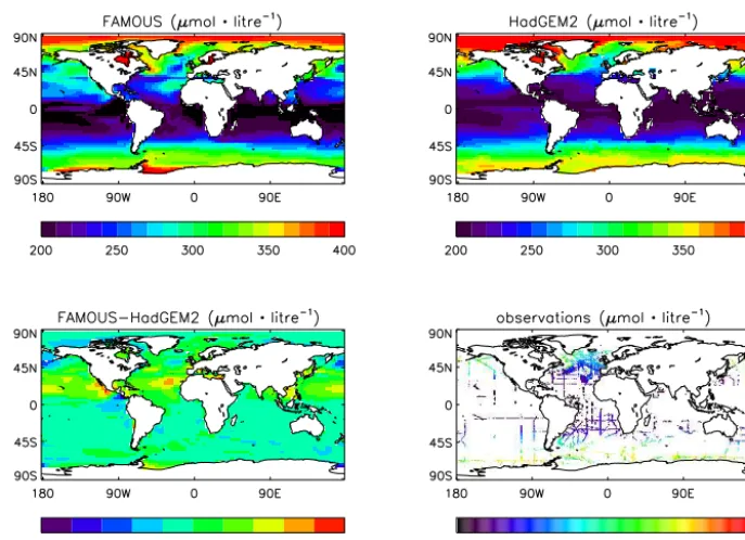
Figure 1. Surface oxygen concentrations (µmol kg−1) for FAMOUS (top left) and HadGEM2-ES (top right). The percentage difference between the two is shown in the bottom left panel and the paucity of observations (Helm et al., 2011) is illustrated in the bottom right panel.

290 parts per million (ppm). The results therefore are repre-sentative of preindustrial boundary conditions. The bound-ary condition files used for initialising the simulation are themselves the result of an equilibrated simulation and there-fore the results presented here can be considered as equi-librated as possible. This simulation uses dynamic vegeta-tion, a complex land-surface exchange scheme and a fully dynamic NPZD (nutrient, phytoplankton, zooplankton, de-tritus) ocean carbon cycle. Detailed model setup information can be found Williams et al. (2013), which describes the per-turbed physics optimisation process used for obtaining the models’ terrestrial and oceanic carbon cycle parameters.

In the next section, agreement between FAMOUS and HadGEM2-ES is described. The horizontal resolution of the ocean GCM in HadGEM2-ES is 1◦ in the east–west plane. The same is true in the north–south plane but only between the poles and 30◦ from where the resolution increases to 0.33◦on the equator. FAMOUS has a global grid spacing of 2.5◦×3.75◦and therefore has almost an order of magnitude reduction in areal resolution. HadGEM2-ES also has twice as many levels in the vertical (40) compared to FAMOUS (20).

3 Validation

FAMOUS was originally developed to act as an interme-diary between complex (and slow running) fully coupled GCMs and fast running (but low complexity) Earth Models of Intermediate Complexity (EMICS). The original reason for the simulator moniker is best quoted from the original

FAMOUS documentation paper of Jones et al. (2005): “Basing FAMOUS on HadCM3 means its results are di-rectly traceable to the state-of-the-art model used for policy-relevant climate projections”.

Since the addition of an oxygen cycle to the ocean com-ponent of FAMOUS represents a completely new addition to the FAMOUS model (and HadCM3 family) it was deemed appropriate to compare the newly obtained climate model output to equivalent data from HadGEM2-ES, the main cli-mate model used by the Met Office Hadley Centre in their submission to the Intergovernmental Panel Climate Change’s fifth assessment report. These data are freely available online from the Programme for Climate Model Diagnosis and Inter-comparison at http://pcmdi9.llnl.gov/esgf-web-fe/.

Figure 1 shows the predicted surface oxygen concentra-tions for FAMOUS and HadGEM2-ES as well as the obser-vational data from Helm et al. (2011) (note that from this pa-per the 1970 oxygen climatology is used). This observational data set is used due to its recent use in validating the oxygen dynamics of HadGEM2-ES under climate change (Andrews et al., 2013) and hence preserves the traceability of the model development process.

(4)

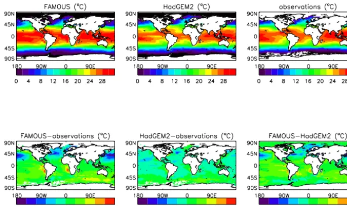
Figure 2. SSTs for FAMOUS (top left), HadGEM2-ES (top middle) and Helm et al. (2011) observations (top right). Difference plots between the models and observations are shown in the bottom left and middle left panels and the difference between the models themselves is shown in the bottom right.

the observations are not a useful benchmark for this latitude– longitude comparison.

Oxygen solubility is a strong negative function of temper-ature as is evident from Fig. 1 which shows (almost zonally symmetric) high values at the poles and lower values at the equator. It is therefore instructive to consider the sea surface temperature (SST) structure of the models and observations. This is shown in Fig. 2. The observational data set is the 1965–1975 decadal mean from Rayner et al. (2003). This meaning period has been used so that the best match with the 1970 oxygen climatology can be obtained. It should be noted however that in this analysis decadal mean SSTs from 1870 to 1880 right up to the present day have been used and the results obtained are qualitatively identical although clearly there are some minor regional differences.

The most striking aspect of the temperature difference be-tween FAMOUS and HadGEM2-ES in Fig. 2 is the consis-tent underestimation of Northern Hemisphere SSTs. This is in agreement with the previously noted (e.g. Williams et al., 2013) Northern Hemisphere cold bias in FAMOUS. Due to the negative correlation between temperature and oxygen solubility, it is expected that the surface oxygen concentra-tion in this region in FAMOUS will generally be higher than in HadGEM2-ES and this is indeed seen in Fig. 1. Clearly there are other effects on surface oxygen concentration such as advection and diffusion of water masses and consumption and generation of oxygen through biogeochemical processes in the surface waters, and these processes are considered be-low. However, the general pattern seen here is in line with first-order thermodynamic expectations.

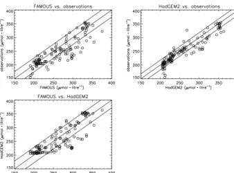
The statistical relationship between simulated and ob-served surface oxygen concentrations is studied by sampling

only the data points in Fig. 1 where observational data from Helm et al. (2011) are present. These plots are shown in Fig. 3.

From Fig. 3 it is clear that FAMOUS generally overesti-mates the observed values. The average value of this differ-ence is 14.5±25.5 µmol L−1where the error estimate is one standard deviation (σ). The equivalent value for HadGEM2-ES vs. observations is 8.3±17.7 µmol L−1 and therefore HadGEM2-ES not only gives a closer fit to the observed val-ues but a more consistently varying one (i.e. lower standard deviation). The comparison of FAMOUS and HadGEM2-ES gives a value of 6.2±28.1 µmol L−1(FAMOUS greater than HadGEM2-ES).

Figure 2 shows that there are some regions where the models’ representation of SST differ significantly and so it is of interest to consider only areas where the mod-els are in relative agreement. To this end the data have been further sub-sampled to include only areas where the models disagree by 2◦_{C or less. The value for the} com-parison between FAMOUS and observations is now 9.9±

24.7 µmol L−1, i.e. a decrease of 32 % in the average dif-ference but only a marginal decrease in the variability. The results for HadGEM2-ES compared to observations are now 8.2±17.4 µmol L−1which are virtually unchanged with re-spect to previous results. This value of 2◦C was chosen be-cause it is the width of the colour contours in Fig. 2. How-ever, choosing either 1 or 3◦C to make this point does not change the conclusion reached.

(5)

Figure 3. Scatter plots showing the relationships between simulated and observed (Helm et al., 2011) surface oxygen concentrations. Data have been sampled so that only data points where observational data are available are shown (Fig. 1, bottom right). The three lines show the 1:1 line and±1 standard deviation (1σ) of the difference between the two quantities.

agreement of HadGEM2-ES with observations in the first place. The essentially unchanged results in the HadGEM2-ES comparison with observations are further proof of this fact, i.e. the points which are discarded in this secondary analysis represent points which are indicative of FAMOUS’ lack of agreement with observations. Whilst this analysis does give results which are intuitively correct, the highly sparse nature of oxygen observations (Fig. 1) makes this analysis of model agreement with observations virtually im-possible “by eye”. The same point holds for the SST data (which are also sparse for this time period, as mentioned above) although they are presented in an interpolated format in the Rayner at al. (2003) data set.

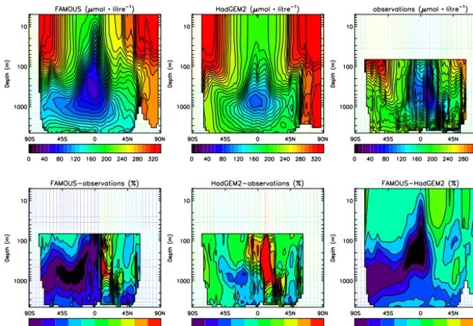
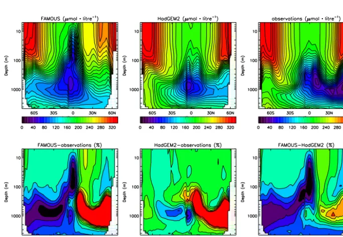
Figure 4 shows the comparison in a zonal mean-depth sense where the observations can provide a useful target for validation. The observed oxygen data in Fig. 4 have a vertical resolution of 50 m throughout the water column.

Firstly, considering the agreement between the models, it is clear that, qualitatively, the oxygen structure of FAMOUS is in good agreement with HadGEM2-ES although the oxy-gen maxima at high northern latitudes are somewhat under-estimated in FAMOUS.

The main area of disagreement in Fig. 4 – both between the models and between the respective models and the ob-servations – is at depth in the Southern Hemisphere where FAMOUS significantly underestimates the oxygen concen-tration.

To examine this issue further, it is necessary to consider both the continuity (i.e. oxygen “amount”) of sinking organic

matter in the model as well as the ocean overturning be-cause this will ultimately affect whether or not surface oxy-gen will be transported to depth. Both of these effects are now considered in turn. Equation (9) is from Palmer and Totterdell (2001) and gives the concentration of detritus as a function of time:

∂D ∂t

_biology

=mDP2+ 1 3

µ1Z+µ2Z2

+ED−λD−Gd, (9) where

mD=m·min

1,Cp Cd

(10) and

ED=

min Gp+Gd−Gz,

CpGp+CdGd−CzGz Cd

!

. (11)

In these preceding three equations,D,P andZ are the de-tritus, phytoplankton and zooplankton concentrations, mD is the phytoplankton mortality rate constant, µ1,2 are the constant and zooplankton-dependent mortality coefficients,

(6)

Figure 4. Zonal mean-depth oxygen concentrations (µmol L−1) for FAMOUS (top left), HadGEM2-ES (top middle) and Helm et al. (2011) observations (top right). Percentage difference plots between the models and observations are shown in the bottom left and middle left panels and the difference between the models themselves is shown in the bottom right.

grazing rates of zooplankton on detritus and phytoplankton respectively. Finally,

m=

(

0, P ≤0.01 µmol L−1, m0, otherwise,

(12)

wherem0is the mortality rate of phytoplankton.

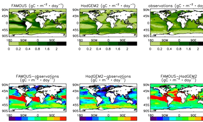
Figure 5 shows the surface net primary productivity (NPP) for FAMOUS and HadGEM2-ES compared to available ob-servations (Behrenfeld and Falkowski, 1997).

Figure 5 clearly shows that both models overestimate equatorial NPP. This overestimation is largest in the Pacific and is significantly larger in FAMOUS. This behaviour has been noted previously in Williams et al. (2013) where the current setup of FAMOUS was compared to previous incar-nations. The tuning target in the perturbed-physics ensembles in Williams et al. (2013) was the surface nitrate concentra-tion, not NPP. It is likely that if NPP had been used instead that this significant equatorial bloom would have been less marked. This spike in productivity will lead to an increased amount of detritus sinking out of the photic zone (top few hundred metres) of the ocean which will then undergo rem-ineralisation. This is qualitatively the reverse of photosyn-thesis and therefore consumes oxygen, hence reducing the oxygen content.

The agreement between simulated and observed oxy-gen concentration is now examined on the basin scale in Figs. 6 and 7 using the spatially complete World Ocean At-las (2009) database (Garcia et al., 2010). It is particularly clear from Fig. 7 that the globally prevalent positive bias in

both FAMOUS and HadGEM2-ES (Fig. 4) between≈100– 1000 m at low northern latitudes can be attributed to the Pa-cific Ocean where the same characteristic “U”-shaped posi-tive bias is evident in both models. Using the reverse of the argument given above, this can be attributed to both models’ underestimation of NPP at mid-to-high latitudes. In Fig. 7, FAMOUS’ pronounced equatorial oxygen minimum can be seen to be due to the equally pronounced NPP maximum at this location. It should be noted here that although a differ-ent data set is used for this part of the analysis, Figs. 6 and 7 have been replotted (not shown) and no significant differ-ences between them was noted. Indeed, as stated above, the reason why the Helm et al. (2011) data set was chosen in the first place was to maintain model development traceability with Andrews et al. (2013). It should also be noted that al-though the World Ocean Atlas oxygen data set does provide a full latitude–longitude data set, the observations that en-ter into it are still sparse, as can be seen from Fig. 8. Indeed it is clear from this figure that although the North Atlantic sector’s coastal regions, the west coast of America and also Japan have very good coverage, significant areas of the world are very poorly sampled – for example virtually the entire Southern Hemisphere.

(7)

Figure 5. Net primary productivity (NPP) (gC m−2day−1) for FAMOUS (top left), HadGEM2-ES (top middle) and observations (top right). Absolute difference plots between the models and observations are shown in the bottom left and middle left panels and the difference between the models themselves is shown in the bottom right.

agreement between observed and simulated NPP and oxygen fields.

The first-order connection between increased (decreased) NPP and decreased (increased) oxygen concentrations holds well throughout this analysis with the only notable exception being the northern Atlantic basin in HadGEM2-ES. In this region, HadGEM2-ES significantly underestimates observed NPP yet has a generally good representation of oxygen.

As stated above, the amount of oxygen produced and con-sumed is one factor in a dynamic system’s behaviour, but for a full understanding, the transport must also be considered. Equation (13) shows the three-dimensional continuity equa-tion for a generic densityρand velocity vector fieldu:

∂ρ

∂t + ∇ ·(ρu)+G + O−G

−

O=0, (13)

whereG+_OandG−_Orepresent generation and consumption of oxygen due to, for example, photosynthesis and remineral-isation. Figures 9 and 10 show the meridional overturning circulation (MOC) in sverdrups (millions of cubic metres per second) for FAMOUS and HadGEM2-ES in the global and Atlantic oceans respectively (note the different latitude limits in the two figures).

From Fig. 9, it is clear that FAMOUS significantly under-estimates the circulation seen in HadGEM2-ES and also fails to reproduce the observed global “two cell” meridional over-turning circulation pattern (for example, Fig. 2 in Lumpkin and Speer, 2007). Assuming that this circulation has an im-portant effect on the oxygen concentration through reduced ventilation, the significantly reduced Southern Hemisphere circulation in FAMOUS compared to HadGEM2-ES should

result in a large decrease in the oxygen concentration in this region, which is indeed seen in Fig. 4.

From a more quantitative angle, the overturning on the basin scale is now interrogated. Kanzow et al. (2010) have given an observed value of 18.7±2.7 Sv for the maximum absolute value of the Atlantic basin overturning at 26.5◦N. For the four HadGEM2-ES realisations studied here (the re-sults presented above are the ensemble mean) a value of 12.7±0.6 Sv is found and for FAMOUS, 12.7±0.4 Sv. The uncertainty estimate in FAMOUS is obtained by calculating the overturning for the last four 30-year periods of a 3500-year run. These figures are in agreement with previously pub-lished data on HadGEM2-ES from the HadGEM2 Develop-ment Team (2011), (13.3±1.0 Sv at 26◦N for a preindustrial simulation) but are weaker than the 2004–2008 estimate of Kanzow et al. (2010) given above and the HadGEM2-ES fig-ures for the period 1990–2000 (16.0±1.0 Sv at 30◦N) from the HadGEM2 Development Team (2011).

Figure 10 shows that HadGEM2-ES has well-developed upper and lower circulatory cells which are analogous to the (upper) North Atlantic Deep Water (NADW) and (lower) Antarctic Bottom Water (AABW) systems observed in Talley et al. (2003). This AABW water cell in the Atlantic basin is not present in FAMOUS. This shows that Southern Hemi-sphere water is not being circulated into northern latitudes and hence that the general circulation in this region is more sluggish than HadGEM2-ES and adds further evidence that the circulation in FAMOUS is being underestimated com-pared to HadGEM2-ES.

(8)

Figure 6. Zonal mean-depth oxygen concentrations for the Atlantic (µmol L−1) for FAMOUS (top left), HadGEM2-ES (top middle) and World Ocean Atlas observations (top right). Percentage difference plots between the models and observations are shown in the bottom left and middle left panels and the difference between the models themselves is shown in the bottom right. The same contour levels as Fig. 4 are deliberately used here and hence the bottom left and bottom right figures show colour saturation due to the evident disagreement. The minimum values are−89 and−92.1 % in the left and right cases respectively.

(9)

Figure 8. The number of observations making up the World Ocean Atlas oxygen climatology (Garcia et al., 2010).

It is hoped that this ongoing work will significantly improve the understanding of deep water formation in the Southern Hemisphere and hence also improve the agreement with ob-servations of oxygen content. FAMOUS has a dynamic sea ice model and static ice sheets over Antarctica and since cryospheric processes have a strong influence on deep water formation, simulations of warm past climates are expected to yield more useful representations of deep water masses due to their lack of permanent ice on land or at sea (e.g. MacLeod et al., 2013). In contrast to the lack of agreement between simulated and observed values at depth, it is clear from Fig. 1 that FAMOUS can provide a good reproduction of the near-surface oxygen distribution predicted by HadGEM2-ES. What this means is that FAMOUS could be used to study long-term future climate scenarios where ocean warming is predicted to exacerbate the already-detected deoxygenation of the oceans due to climate change (e.g. Andrews et al., 2013). These future scenarios should be confined to surface waters due to the already-mentioned issues with the model reproduction of observed oxygen at depth. However, it is only in the first≈100 m where light can penetrate far enough to stimulate primary production and hence serve as the base of the ocean food chain.

Now, considering the Atlantic basin as a whole, the nu-merical information of Talley et al. (2003) is given in Table 1 along with the data for 26.5◦N given above (note that Fig. 10 gives the maximum Atlantic overturning value for FAMOUS at approximately 26◦N). The lower value for FAMOUS com-pared to HadGEM2-ES is in agreement with the results noted above, i.e. that the circulation in FAMOUS is generally more sluggish than HadGEM2-ES. The fact that both models un-derestimate the value of 18 Sv given by Talley et al. however should be tempered by the fact that the authors give an error estimate of between 3 and 5 Sv on their circulation magni-tudes.

For completeness, the circulation pattern in the Pacific basin is now considered and is shown in Fig. 11. As has been previously shown for the Atlantic basin, the circulation in the

Figure 9. Global meridional overturning circulation (MOC) in FA-MOUS (left) and HadGEM2-ES (right). The zero contour is dashed.

Figure 10. Atlantic meridional overturning circulation (MOC) in FAMOUS (left) and HadGEM2-ES (right). The zero contour is dashed.

(10)

Table 1. Atlantic meridional overturning circulation (AMOC) in Sv for the Atlantic on the basin scale (lower line) and specifically at 26.5◦N (upper line). Note the lack of an error estimate for the Talley et al. (2003) figures. The authors of this paper note “Uncertainty in the diagnosed streamfunction is large, on the order of 3–5 Sv”.

FAMOUS HadGEM2-ES Kanzow et al. (2010) Talley et al. (2003)

Atlantic (26.5◦N) 12.7±0.4 12.7±0.6 18.7±2.7 –

Atlantic (basin scale) 12.7±0.4 15.0±0.9 – 18

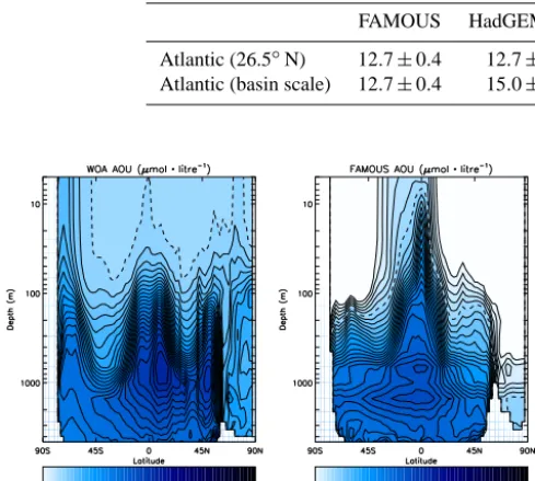
Figure 12. Global apparent oxygen utilisation for World Ocean At-las observations (left) and for FAMOUS (right). The zero contour is dashed.

Pacific for FAMOUS is noticeably weaker than HadGEM2-ES. However, unlike in the Atlantic basin, FAMOUS does show some Southern Hemisphere deep water formation. This may help to explain the reduced (yet still notable) oxygen un-derestimation in Fig. 7 compared to Fig. 6, i.e. the deep wa-ter formation is providing increased pelagic ventilation and hence increased oxygen concentration.

Finally, the apparent oxygen utilisation (AOU) is consid-ered. This is a measure of the biochemically induced devia-tion of oceanic oxygen from its equilibrium atmospheric con-centration (e.g Garcia et al., 2010) and is shown for World Ocean Atlas observations and FAMOUS in Figs. 12–14. As can be seen on a global scale from Fig. 12, FAMOUS has large negative values at the surface, particularly at mid-to-high latitudes. What this means is that the surface ocean is over-saturated with oxygen. Interestingly, it can also be seen from Fig. 14 that FAMOUS’ global structure in Fig. 12 can mostly be attributed to the Pacific. This makes sense because (as can be seen in Fig. 5) although FAMOUS generally over-estimates equatorial NPP, the Pacific bias clearly dominates. Now considering the Atlantic AOU, the correlation be-tween FAMOUS’ oxygen concentration (with respect to ob-servations) in Fig. 6 and the AOU in Fig. 13 is striking, par-ticularly in the Northern Hemisphere. What this means is that the AOU in the north Atlantic is significantly too high (large negative values) because of enhanced photosynthesis. However this is being compensated by other processes, for

Figure 13. Apparent oxygen utilisation for the Atlantic; World Ocean Atlas observations (left) and for FAMOUS (right). The zero contour is dashed.

Figure 14. Apparent oxygen utilisation for the Pacific; World Ocean Atlas observations (left) and for FAMOUS (right). The zero contour is dashed.

example the lack of deep water mixing (Fig. 10). This com-pensation of one process being overestimated and (at least) one being underestimated combine to give good agreement at high northern latitudes (Fig. 6).

(11)

fundamentally in this example, that the oxygen scheme de-scribed here is an addition to a pre-existing NPZD model. This can, for example, be contrasted to the Darwin model (e.g. Vallina et al., 2014) which can represent not only many functional forms of plankton but also their adaptation to en-vironmental niches.

4 Conclusions

This paper describes an update to the latest version of FA-MOUS (Williams et al., 2013) in which a numerically calcu-lated oxygen cycle is included for the first time. This follows the scheme of the latest Hadley Centre GCM, HadGEM2-ES, under the auspices of the second phase of the Ocean Carbon-Cycle Model Intercomparison Project, OCMIP2. The sur-face oxygen concentration is in good agreement with that of HadGEM2-ES. FAMOUS’ general overestimation of the Northern Hemisphere surface oxygen concentration is at-tributed to its underestimation of SST. When the model out-put is compared against available surface observations on a point-by-point basis, both models generally overestimate the observed values, although this overestimation is reduced in HadGEM2-ES.

The agreement between the simulated oxygen concentra-tions at depth in the Northern Hemisphere is also encourag-ing. The deep Southern Hemisphere agreement is less good however.

The notable disagreement between oxygen concentrations at depth in the Southern Hemisphere is partially ascribed to FAMOUS’ overestimation of equatorial net primary pro-ductivity which causes increased remineralisation of sink-ing detritus at depth and hence increased oxygen consump-tion. This is further exacerbated by reduced ocean circula-tion in FAMOUS compared to HadGEM2-ES which acts to reduce Southern Hemisphere ventilation. This reduction in circulatory strength is evident in both the global and Atlantic oceans. To aid regional understanding in this regard, merid-ional overturning circulation, oxygen concentrations and ap-parent oxygen utilisation (AOU) have been studied on the basin scale. Examples of the utility of this include the attri-bution of Northern Hemisphere, intermediate depth overes-timation of oxygen in both HadGEM2-ES and FAMOUS to the Pacific and also give an explanation of why equatorial blooms of NPP seem to affect the deep oxygen concentra-tion in the Southern Hemisphere more than in the Northern Hemisphere in FAMOUS.

Finally, the authors feel that with recent developments in the terrestrial and oceanic carbon cycles and now with the in-troduction of oceanic oxygen, the FAMOUS model is leaving the traditional “climate model” definition and moving into the realm of an “Earth-System model” – hence the title of this paper.

Code availability

The main repository for the Met Office Unified Model (UM) at the version corresponding to the model presented here can be found at http://cms.ncas.ac.uk/code_browsers/UM4. 5/UMbrowser/index.html.

Supplement

The code detailing the advances described in this paper is completely contained within one text file (known as a code modification file or “mod”) and this is available as a Supple-ment to this paper. This is protected under Crown Copyright, as is the base code linked above.

The Supplement related to this article is available online at doi:10.5194/gmd-7-1419-2014-supplement.

Acknowledgements. J. H. T. Williams and P. J. Valdes were supported by funding from Statoil ASA, Norway. J. H. T. Williams and P. J. Valdes thank T. L. Leith of Statoil ASA for extensive discussions throughout this work. I. J. Totterdell and P. R. Halloran were supported by the Joint DECC/Defra Met Office Hadley Centre Climate Programme (GA01101). The authors are grateful to two anonymous reviewers and to the topical editor whose comments and suggestions have significantly improved this paper.

Edited by: G. Munhoven

References

Andrews, O. D., Bindoff, N. L., Halloran, P. R., Ilyina, T., and Le Quéré, C.: Detecting an external influence on recent changes in oceanic oxygen using an optimal fingerprinting method, Biogeo-sciences, 10, 1799–1813, doi:10.5194/bg-10-1799-2013, 2013. Anderson, L. A. and Sarmiento, J. L.: Redfield ratios of

rem-ineralization determined by nutrient data analysis, Global Bio-geochem. Cy., 8, 65–80, 1994

Behrenfeld, M. J. and Falkowski, P. G.: Photosynthetic rates de-rived from satellite-based chlorophyll concentration, Limnol. Oceanogr., 42, 1–20, 1997.

Bellouin, N., Rae, J., Jones, A., Johnson, C., Haywood, J., and Boucher, O.: Aerosol forcing in the climate model intercom-parison project (CMIP5) simulations by HadGEM2-ES and the role of ammonium nitrate, J. Geophys. Res., 116, D20206, doi:10.1029/2011JD016074, 2011.

Bopp, L., Le Quéré, C., Heimann, M., and Manning, A. C.: Climate-induced oceanic oxygen fluxes: Implications for the contem-porary carbon budget, Global Biogeochem. Cy., 16, 6.1–6.13, doi:10.1029/2001GB001445, 2002.

(12)

S., Totterdell, I., Wiltshire, A., and Woodward, S.: Develop-ment and evaluation of an Earth-System model – HadGEM2, Geosci. Model Dev., 4, 1051–1075, doi:10.5194/gmd-4-1051-2011, 2011.

Cox, P. M., Betts, R. A., Jones, C. D., Spall, S. A., and Totter-dell, I. J.: Acceleration of global warming due to carbon-cycle feedbacks in a coupled climate model, Nature, 408, 184–187, 2000.

Frölicher, T. L., Joos, F., Plattner, G.-K., Steinacher, M., and Doney, S. C.: Natural variability and anthropogenic trends in oceanic oxygen in a coupled carbon–climate model ensemble, Global Biogeochem. Cy., 23, GB1003, doi:10.1029/2008GB003316, 2009.

Garcia, H. E. and Gordon, L. I.: Oxygen solubility in seawater: bet-ter fitting equations, Limnol. Oceanogr., 37, 1307–1312, 1992. Garcia, H. E., Locarnini, R. A., Boyer, T. P., Antonov, J. I.,

Bara-nova, O. K., Zweng, M. M., and Johnson, D. R.: World Ocean Atlas 2009, Volume 3: Dissolved Oxygen, Apparent Oxygen Uti-lization, and Oxygen Saturation, edited by: Levitus, S., NOAA Atlas NESDIS 70, U.S. Government Printing Office, Washing-ton, D.C., 344 pp., 2010.

Gordon, C., Cooper, C., Senior, C. A., Banks, H., Gregory, J. M., Johns, T. C., Mitchell, J. F. B., and Wood, R. A.: The simulation of SST, sea ice extents and ocean heat transports in a version of the Hadley Centre coupled model without flux adjustments, Clim. Dynam., 16, 147–168, 2000.

The HadGEM2 Development Team: G. M. Martin, Bellouin, N., Collins, W. J., Culverwell, I. D., Halloran, P. R., Hardiman, S. C., Hinton, T. J., Jones, C. D., McDonald, R. E., McLaren, A. J., O’Connor, F. M., Roberts, M. J., Rodriguez, J. M., Woodward, S., Best, M. J., Brooks, M. E., Brown, A. R., Butchart, N., Dear-den, C., Derbyshire, S. H., Dharssi, I., Doutriaux-Boucher, M., Edwards, J. M., Falloon, P. D., Gedney, N., Gray, L. J., Hewitt, H. T., Hobson, M., Huddleston, M. R., Hughes, J., Ineson, S., In-gram, W. J., James, P. M., Johns, T. C., Johnson, C. E., Jones, A., Jones, C. P., Joshi, M. M., Keen, A. B., Liddicoat, S., Lock, A. P., Maidens, A. V., Manners, J. C., Milton, S. F., Rae, J. G. L., Rid-ley, J. K., Sellar, A., Senior, C. A., Totterdell, I. J., Verhoef, A., Vidale, P. L., and Wiltshire, A.: The HadGEM2 family of Met Of-fice Unified Model climate configurations, Geosci. Model Dev., 4, 723–757, doi:10.5194/gmd-4-723-2011, 2011.

Helm, K. P., Bindoff, N. L., and Chrusch, J. A.: Observed decreases in oxygen content of the global ocean, Geophys. Res. Lett., 38, L23602, doi:10.1029/2011GL049513, 2011.

Hewitt, H. T., Copsey, D., Culverwell, I. D., Harris, C. M., Hill, R. S. R., Keen, A. B., McLaren, A. J., and Hunke, E. C.: Design and implementation of the infrastructure of HadGEM3: the next-generation Met Office climate modelling system, Geosci. Model Dev., 4, 223–253, doi:10.5194/gmd-4-223-2011, 2011.

Jones, C., Gregory, J., Thorpe, R., Cox, P., Murphy, J., Sexton, D., and Valdes, P.: Systematic optimisation and climate simulations of FAMOUS, a fast version of HadCM3, Clim. Dynam., 25, 189– 204, 2005.

Kanzow, T., Cunningham, S. A., Johns, W. E., Hirschi, J. J.-M., Marotzke, J., Baringer, M. O., Meinen, C. S., Chidichimo, M. P., Atkinson, C., Beal, L. M., Bryden, H. L., and Collins, J.: Sea-sonal variability of the Atlantic meridional overturning circula-tion at 26.5◦N, J. Climate, 23, 5678–5698, 2010.

Keeling, R. F., Stephens, B. B., Najjar, R. G., Doney, S. C., Archer, D., and Hemimann M.: Seasonal variations in the atmospheric O₂/ N₂ratio in relation to the kinetics of air–sea gas exchange, Global Biogeochem. Cy., 12, 141–163, 1998.

Lumpkin, R. and Speer, K.: Global ocean meridional circulation, J. Phys. Oceanogr., 37, 2550–2562, 2007.

Macleod, K. G., Huber, B. T., Berrocoso, Á. J., and Wendler, I.: A stable and hot Turonian with glacialδ18O excursions is indicated by exquisitely preserved Tanzanian foraminifera, Geology, 41, 1083–1086, 2013.

Martin, G. M., Ringer, M. A., Pope, V. D., Jones, A., Dear-den, C., and Hinton, T. J.: The physical properties of the atmo-sphere in the new Hadley Centre Global Environmental Model (HadGEM1) – Part 1: Model description and global climatol-ogy, J. Climate, 19, 1274–1301, 2006.

Matear, R. J., Hirst, A. C., and McNeil, B. I.: Changes in dissolved oxygen in the Southern Ocean with climate change, Geochem. Geophy. Geosy., 1, 1050, doi:10.1029/2000GC000086, 2000. Monteiro, F. M., Pancost, R. D., Ridgwell, A., and Donnadieu, Y.:

Nutrients as the dominant control on the spread of anoxia and euxinia across the Cenomanian-Turonian ocean anoxic event (OAE2): model-data comparison, Paleoceanography, 27, PA4209, doi:10.1029/2012PA002351, 2012.

Najjar, R. G. and Orr, J. C.: Biotic-HOWTO revision 1.7, OCMIP technical document, last edited: 5 October 1999, available at: www.cgd.ucar.edu/oce/OCMIP/HOWTO-Biotic.ps (last access: 6 June 2014), 1999.

Palmer, J. R. and Totterdell, I. J.: Production and export in a global ocean ecosystem model, Deep-Sea Res. Pt. I, 48, 1169–1198, 2001.

Peña, M. A., Katsev, S., Oguz, T., and Gilbert, D.: Modeling dis-solved oxygen dynamics and hypoxia, Biogeosciences, 7, 933– 957, doi:10.5194/bg-7-933-2010, 2010.

Pope, V. D., Gallani, M. L., Rowntree, P. R., and Stratton, R. A.: The impact of new physical parametrizations in the Hadley Centre climate model: HadAM3, Clim. Dynam., 16, 123–146, 2000. Rayner, N. A., Parker, D. E., Horton, E. B., Folland, C. K.,

Alexan-der, L. V., Rowell, D. P., Kent, E. C., and Kaplan, A.: Global analyses of sea surface temperature, sea ice, and night marine air temperature since the late nineteenth century, J. Geophys. Res., 108, 4407, doi:10.1029/2002JD002670, 2003.

Reichler, T. and Kim, J.: How well do coupled models simu-late today’s climate?, B. Am. Meteorol. Soc., 89, 303–311, doi:10.1175/BAMS-89-3-303, 2008.

Smith, R. S.: The FAMOUS climate model (versions XFXWB and XFHCC): description update to version XDBUA, Geosci. Model Dev., 5, 269–276, doi:10.5194/gmd-5-269-2012, 2012.

Smith, R. S., Gregory, J. M., and Osprey, A.: A description of the FAMOUS (version XDBUA) climate model and control run, Geosci. Model Dev., 1, 53–68, doi:10.5194/gmd-1-53-2008, 2008.

Talley, L. D., Reid, J. L., and Robbins, P. E.: Data-based meridional overturning streamfunctions for the global ocean, J. Climate, 16, 3213–3226, 2003.

(13)

Webb, M., Senior, C., Bony, S., and Morcrette, J.-J.: Combining ERBE and ISCCP data to assess clouds in the Hadley Centre, ECMWF and LMD atmospheric climate models, Clim. Dynam., 17, 905–922, 2001.