An automatic and effective parameter optimization method for model tuning

(1)

www.geosci-model-dev.net/8/3579/2015/ doi:10.5194/gmd-8-3579-2015

An automatic and effective parameter optimization method for

model tuning

T. Zhang1,2, L. Li3, Y. Lin2, W. Xue1,2, F. Xie3, H. Xu1, and X. Huang1,2

1_{Department of Computer Science and Technology, Tsinghua University, Beijing 100084, China}

2_{Center for Earth System Science, Ministry of Education Key Laboratory for Earth System Modeling, Tsinghua University,} Beijing 100084, China

3_{State Key Laboratory of Numerical Modeling for Atmospheric Sciences and Geophysical Fluid Dynamics,} Institute of Atmospheric Physics, Chinese Academy of Sciences, Beijing 100029, China

Correspondence to: W. Xue ([email protected]) and L. Li ([email protected]) Received: 7 April 2015 – Published in Geosci. Model Dev. Discuss.: 7 May 2015

Revised: 27 August 2015 – Accepted: 9 October 2015 – Published: 6 November 2015

Abstract. Physical parameterizations in general circula-tion models (GCMs), having various uncertain parameters, greatly impact model performance and model climate sensi-tivity. Traditional manual and empirical tuning of these pa-rameters is time-consuming and ineffective. In this study, a “three-step” methodology is proposed to automatically and effectively obtain the optimum combination of some key pa-rameters in cloud and convective parameterizations accord-ing to a comprehensive objective evaluation metrics. Dif-ferent from the traditional optimization methods, two extra steps, one determining the model’s sensitivity to the param-eters and the other choosing the optimum initial value for those sensitive parameters, are introduced before the down-hill simplex method. This new method reduces the number of parameters to be tuned and accelerates the convergence of the downhill simplex method. Atmospheric GCM simulation re-sults show that the optimum combination of these parameters determined using this method is able to improve the model’s overall performance by 9 %. The proposed methodology and software framework can be easily applied to other GCMs to speed up the model development process, especially regard-ing unavoidable comprehensive parameter tunregard-ing durregard-ing the model development stage.

1 Introduction

Due to their current relatively low model resolutions, gen-eral circulation models (GCMs) need to parameterize vari-ous sub-grid-scale processes. Physical parameterizations aim to approximate the overall statistical outcomes of various sub-grid-scale physics (Williams, 2005). However, due to the complexities involved in these processes, parameteriza-tions representing sub-grid-scale physical processes unavoid-ably involve some empirical or statistical parameters (Hack et al., 1994), especially within cloud and convective parame-terizations. Consequently, these parameterizations introduce uncertainties into climate simulations using GCMs (Warren and Schneider, 1979). In general, these uncertain parameters need to be calibrated or constrained when new parameteriza-tion schemes are developed and integrated into models (L. Li et al., 2013).

(2)

For the PDF method, the confidence ranges of the opti-mization parameters are evaluated based on likelihood and Bayesian estimation. Cameron et al. (1999) approximate the forecast by the generalized likelihood uncertain estimation (Beven and Binley, 1992), a method obtaining parameter un-certainty ranges of a specific confidence level. The Bayesian Markov chain Monte Carlo (MCMC) method (Gilks, 1995) is widely used to obtain posterior probability distributions from prior knowledge. A couple of specific algorithms based on the MCMC theory are used to calibrate models in the previous literatures, such as Metropolis–Hasting (Sun et al., 2013), the adaptive Metropolis algorithm (Hararuk et al., 2014), and multiple very fast simulated annealing (MVFSA) (Jackson et al., 2008). The MVFSA method is 1 to 2 orders of magnitude faster than the Metropolis–Hasting al-gorithm (Jackson et al., 2004). However, these methods only attempt to determine the most likely area of uncertain param-eters and cannot directly give the best combination of uncer-tain parameters with an optimum metrics value. Moreover, the PDF heavily depends on the likelihood function assumed, which is usually difficult to determine for climate system model tuning problems.

Optimization algorithms can be used to search the maxi-mum or minimaxi-mum metrics value in a given parametric space. Severijns and Hazeleger (2005) calibrate parameters of radi-ation, clouds, and convection in the Speedy model with the downhill simplex (Press et al., 1992; Nelder and Mead, 1965) to improve the radiation budget at the top of the atmosphere and at the surface, as well as the large-scale circulation. The downhill simplex is a fast convergence algorithm when the parametric space is not high-dimensional. However, it is a lo-cal optimization algorithm, not aiming to find the global op-timal solution. Moreover, the algorithm has convergence is-sues when the simplex becomes ill-conditioned. Besides the downhill simplex, a few global optimization algorithms are introduced to tune uncertain parameters of climate system models, such as simulated stochastic approximation anneal-ing (SSRR) (Yang et al., 2013), MVFSA (Yang et al., 2014), and multi-objective particle swarm optimization (MOPSO) (Gill et al., 2006). SSRR requires at least 10 000 steps to get a stable solution (Liang et al., 2013), and MVFSA also re-quires thousands of steps to get a stable solution (Jackson et al., 2004). MOPSO needs dozens of individual cases in each iteration. All these global optimization algorithms re-quire a large number of model runs and very high computa-tional cost during the model tuning process.

The data assimilation method has been well addressed for state estimation, and can be a potential solution for param-eter estimation. Aksoy et al. (2006) estimates the paramparam-eter uncertainty in a mesoscale model (Grell et al., 1994) using the ensemble Kalman filter (EnKF). Santitissadeekorn and Jones (2015) presents a two-step filtering for the joint state parameter estimation with a combination method of particle filtering (PF) and EnKF. The EnKF and PF use an ensem-ble of model simulations to estimate the background error

covariance, which approximate the traditional Kalman fil-ter with a recurrence process (Evensen, 2003; Arulampalam et al., 2002). The accuracy of the error covariance relies on samples. In general, the larger the ensemble size, the more accurate the estimates are. The limitation of ensemble size for practice use and imperfect models make it difficult to se-lect representative samples (Poterjoy et al., 2014). Moreover, as with the MOPSO method, they require a large number of model runs in each iteration with greatly increased computa-tional cost.

A climate system model is a strongly nonlinear system, having a large number of uncertain parameters. As a re-sult, the parametric space of a climate system model is high-dimensional, multi-modal, strongly nonlinear, and insepara-ble. More seriously, one model run of a climate system model might require tens or even hundreds of years of simulation to get scientifically meaningful results.

To overcome these challenges, we propose a “three-step” strategy to calibrate the uncertain parameters in climate system models effectively and efficiently. First, the Morris method (Morris, 1991; Campolongo et al., 2007), a global sensitivity analysis method, is chosen to eliminate the in-sensitive parameters by analyzing the main and interactive effects among parameters. Another global method by Sobol (Sobol, 2001) is used to validate the results of the Morris method. Second, a pre-processing of initial values of selected parameters is presented to accelerate the convergence of opti-mization algorithm and to resolve the issue of ill-conditioned problems. Finally, the downhill simplex algorithm is used to solve the optimization problem because of its low computa-tional cost and fast convergence for low-dimensional space. Taking into account the complex configuration and manipu-lation of model tuning, an automatic workflow is designed and implemented to make the calibration process more ef-ficient. The method and workflow can be easily applied to GCMs to speed up model development processes.

The paper is organized as follows. Section 2 introduces the proposed automatic workflow. Section 3 describes the de-tails of the example model, reference data, and calibration metrics. The three-step calibration strategy is presented in Sect. 4. Section 5 evaluates the calibration results, followed by a summary in Sect. 6.

2 The end-to-end automatic calibration workflow

(3)

se-lection, model configuration and running, and evaluation of model outputs using user-provided metrics. Users only need to specify the model to tune, the parameters to be tuned with their valid ranges, and the calibration method to use.

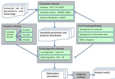
There are four main modules within the framework as shown in Fig. 1. The scheduler module manages model sim-ulations with the capability for simultaneous runs. It also coordinates different tasks to reduce the contention and im-prove throughput. Simulation diagnosis and evaluation are included in a post-processing module. The preparation mod-ule contains various sensitivity analysis and sampling meth-ods, such as the Morris (Morris, 1991; Campolongo et al., 2007), Sobol (Sobol, 2001), full factorial (FF) (Raktoe et al., 1981), Latin hypercube (LH) (McKay et al., 1979), Morris one-at-a-time (MOAT) (Morris, 1991), and central compos-ite designs (CCD) (Hader and Park, 1978) methods. The sen-sitivity analysis is able to eliminate the duplicated samples to reduce unnecessary model runs. A MCMC method based on adaptive Metropolis–Hastings algorithms is also provided to get the posterior distribution of uncertain parameters. The tuning algorithm module offers various local and global opti-mization algorithms including the downhill simplex, genetic algorithm, particle swarm optimization, differential evolu-tion and simulated annealing. In addievolu-tion, all the intermediate metrics and their corresponding parameters within the frame-work are stored in a MySQL database and can be used for posterior knowledge analysis. More importantly, the work-flow is flexible and expandable for easy integration of other advanced algorithms as well as tools like the Problem Solv-ing Environment for Uncertainty Analysis and Design Explo-ration (PSUADE) (Tong, 2005) and the Design Analysis Kit for Optimization and Terascale Applications (DAKOTA) (El-dred et al., 2007). Although uncertainty quantification toolk-its such as PSUADE and DAKOTA support various calibra-tion and uncertainty analysis methods and pre-defined func-tion interfaces, they cannot organize the above model tuning process as effectively as the proposed model tuning frame-work.

3 Model description and reference metrics

We use the Grid-point Atmospheric Model of IAP LASG version 2 (GAMIL2) as an example for the demonstration of the tuning workflow and our calibration strategy. GAMIL2 is the atmospheric component of the Flexible Global–Ocean– Atmosphere–Land System Model grid version 2 (FGOALS-g2), which participated in the CMIP5 (the fifth phase of the Coupled Model Intercomparison Project) program. The horizontal resolution is 2.8◦×2.8◦, with 26 vertical levels. GAMIL2 uses a finite-difference scheme that conserves mass and energy (Wang et al., 2004). A two-step shape-preserving advection scheme (Yu, 1994) is used for tracer advection. Compared to the pervious version, GAMIL2 has modifica-tions in cloud-related processes (L. Li et al., 2013), such as

the deep convection parameterization (Zhang and Mu, 2005), the convective cloud fraction (Xu and Krueger, 1991), the cloud microphysics (Morrison and Gettelman, 2008), and the stratiform fractional cloud condensation scheme (Zhang et al., 2003). More details are in L. Li et al. (2013). Empir-ical tunable parameters are selected from schemes of deep convection, shallow convection, and cloud fraction schemes (Table 1). Default parameter values are from the model con-figuration for CMIP5 experiments.

To save computational cost, atmosphere-only simulations are conducted for 5 years using prescribed seasonal climatol-ogy (no interannual variation) of SST and sea ice. Previous studies have shown that a 5-year type of simulation is enough to capture the basic characteristics of simulated mean climate states (Golaz et al., 2011; Lin et al., 2013). The goal of these simulations is not to determine their resemblance to observa-tions, but to compare the results between the control simula-tion and various tuned simulasimula-tions.

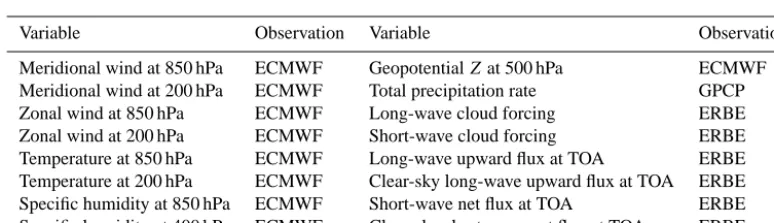
Model tuning results depend on the reference metrics used. For a simple justification, we use some conventional climate variables for the evaluation. Wind, humidity, and geopoten-tial height are from the European Center for Medium-Range Weather Forecasts (ECMWF) Re-Analysis (ERA)–Interim reanalysis from 1989 to 2004 (Simmons et al., 2007). We use the GPCP (Global Precipitation Climatology Project, Adler et al., 2003) for precipitation and the ERBE (Earth Radiation Budget Experiment, Barkstrom, 1984) for radiative fields. All observational and reanalysis data are gridded to the same grid as GAMIL2 before the comparison. Note that the refer-ence metrics can be extended, depending on the model per-formance requirement.

The reference metrics, including various variables in Ta-ble 2, is used to quantitatively evaluate the performance of overall simulation skills (Murphy et al., 2004; Gleckler et al., 2008; Reichler and Kim, 2008). The calibration RMSE is de-fined as the spatial standard deviation (SD) of the model sim-ulation against observations/re-analysis, as in Eq. (1) (Taylor, 2001; Yang et al., 2013). For an easy comparison, we normal-ize the RMSE of each simulation output by that of the con-trol simulation using default parameter values. We introduce an improvement index to evaluate the tuning results, which weight each variable equally and compute the average nor-malized RMSE. The index indicates an overall improvement of the performance of the tuned simulation relative to the control simulation based on a number of model outputs (Ta-ble 2). If the index is less than 1, it means the tuned simula-tion gets better performance than the control run. The smaller this value, the better the improvement is.

(σ_mF)2=

I X i₌1

w(i)(x_mF(i)−x_oF(i))2 (1)

(σ_rF)2=

I X

i=1

(4)

Sensi&vity parameters and posterior distribu&on

Op&miza&on parameters

Analysis results Prepara&on Module

_Sampling_：_{FACT, LHS, MOAT}

Sensi&vity analysis：MORRIS, SOBOL

Posterior distribu&on：MCMC

Tuning algorithm Module

_{Local algorithm}_：_Down-‐hill

Global algorithm：PSO，DE

Diagnose analysis

Post Processing Module

_{Management of results ﬁle}

Management of observa&on data

Metrics diagnose Scheduler Module

Schedule Monitor Recover

Simulate

Simulate Universal set of parameters and ini&al range

Figure 1. The structure of the automatic calibration workflow. The input of the workflow is the parameter set interest and their initial value

ranges. The output is the optimal parameters and their corresponding diagnostic results after calibration. The preparation module provides the parameter sensitivity analysis. The tuning algorithm module offers local and global optimization algorithms including the downhill simplex, genetic algorithm, particle swarm optimization, differential evolution, and simulated annealing. The scheduler module schedules as many as cases to run simultaneously and coordinates different tasks over a parallel system. The post-processing module is responsible for metrics diagnostics, re-analysis and observational data management.

χ2= 1 NF

NF X F₌1

(σ

F

m σF r

)2 (3)

x_mF(i)is the model outputs, andxF_o(i)is the corresponding observation or reanalysis data.x_rF(i)is model outputs from the control simulation using the default values for the param-eters in Table 1.wis the weight due to the different grid area on a regular latitude–longitude grid on the sphere. I is the total grid number in model.NF is the number of the chosen variables.

4 Method

4.1 Parameter tuning with global and local optimization methods

Parameter tuning for a climate system model is intended to solve a global optimization problem in theory. As the well-known global optimization algorithms, traditional evolution-ary algorithms, such as the genetic algorithm (Goldberg et al., 1989), differential evolutionary (DE) (Storn and Price, 1995), and particle swarm optimization (PSO) (Kennedy, 2010) algorithms, can approach the global optimal solution,

but generally require high computational cost (Hegerty et al., 2009; Shi and Eberhart, 1999). This is because these algo-rithms are designed following biological evolution of sur-vival of the fittest. In contrast, the local algorithms utilize the greedy strategy, and thus may tap into a locally optimal solu-tion after convergence. The advantage of local algorithms is the low computational cost due to the relatively fewer sam-ples required. In this sense, the local optimization algorithms are the viable options considering their significantly reduced computational cost.

We choose the downhill simplex method for climate model tuning considering its relatively low computation cost. The downhill simplex method searches the optimal solution by changing the shape of a simplex, which represents the op-timal direction and step length. A simplex is a geometry, consisting ofN+1 vertexes and their interconnecting edges, where N is the number of calibration parameters. One vertex stands for a pair of a set of parameters and their improvement index as defined in Eq. (3). The new vertex is determined by expanding or shrinking the vertex with the highest metrics value, leading to a new simplex (Press et al., 1992; Nelder and Mead, 1965).

(5)

Table 1. A summary of parameters to be tuned in GAMIL2. The default and final tuned optimum values are also shown. The valid range of

each parameter is also included. Note that only four sensitive parameters are tuned and have optimum values.

Parameter Description Default Range Optimal

c0 Rainwater autoconversion coefficient for deep

convection

3.0×10−4 1.×10−4–5.4×10−3 5.427294×10−4

ke Evaporation efficiency for deep convection 7.5×10−6 5×10−7–5×10−5 –

capelmt Threshold value for cape for deep convection 80 20–200 –

rhminl Threshold RH for low clouds 0.915 0.8–0.95 0.917661

rhminh Threshold RH for high clouds 0.78 0.6–0.9 0.6289215

c0_shc Rainwater autoconversion coefficient for shallow

convection

5×10−5 3×10−5–2×10−4 –

cmftau Characteristic adjustment timescale of shallow

capes

7200 900–14 400 7198.048

Table 2. Atmospheric fields included in the evaluation metrics and their sources.

Variable Observation Variable Observation

Meridional wind at 850 hPa ECMWF GeopotentialZat 500 hPa ECMWF

Meridional wind at 200 hPa ECMWF Total precipitation rate GPCP

Zonal wind at 850 hPa ECMWF Long-wave cloud forcing ERBE

Zonal wind at 200 hPa ECMWF Short-wave cloud forcing ERBE

Temperature at 850 hPa ECMWF Long-wave upward flux at TOA ERBE

Temperature at 200 hPa ECMWF Clear-sky long-wave upward flux at TOA ERBE

Specific humidity at 850 hPa ECMWF Short-wave net flux at TOA ERBE

Specific humidity at 400 hPa ECMWF Clear-sky short-wave net flux at TOA ERBE

calibration of climate system models is a balance between model improvement (effectiveness) and computational cost (efficiency). In this study, model improvement is measured by an index defined in Eq. (3). The lower this value is, the better the model tuning is. Computational cost is measured by “core hours”, which stands for the computational effi-ciency. It is computed by(Nstep)×(Nsize)×(the number of processes of a single model run)×(hours used for a single 5-year model run ).Nstepis the total number of iterations of optimization algorithms for convergence.Nsizeis the number of model runs during each iteration, and it is 1 for the down-hill simplex method. In the GAMIL2 case, each model run takes 6 h using 30 processes.

According to tuning GAMIL2, two global methods, PSO and DE, give better tuning effectiveness than the downhill simplex method, but their computational costs are approxi-mately 4 and 5 times, respectively, those of the downhill sim-plex method (Table 3).

To improve the effectiveness of the downhill simplex method, we propose two important steps to significantly im-prove its performance. In the first step, the number of tuning parameters is reduced by eliminating the insensitive parame-ters. In the second step, fast convergence is achieved by pre-selecting proper initial values for the parameters before using the downhill simplex method.

4.2 Parameter sensitivity analysis

The number of uncertain parameters in physical param-eterizations of a climate system model is quite large. Most optimization algorithms, such as PSO, the downhill simplex method, and the simulated annealing algorithm (Van Laarhoven and Aarts, 1987), are ineffective in high-dimensional problems. Iterations for convergence will in-crease exponentially with the number of tuning parameters. In addition, climate models generally need a long simulation to have meaningful results. Therefore, the high-dimensional parameter tuning problem suffers from an extremely high computational cost. It is necessary to reduce the parameter dimension before the optimization.

(6)

Table 3. Effectiveness and efficiency comparison between the original downhill simplex method and the two global methods.Nstep is the

total number of calibrating iterations for convergence.Nsizeis the number of model runs during each iteration. Core hours is computed by

Nstep×Nsize×{the number of processes of a single model run}×{hours used for a single 5-year model run}. In the GAMIL2 case, each

model run takes 6 h and uses 30 processes.

Improvement index Nstep Nsize Core hours

Downhill_1_step 0.9585 80 1 14 400

PSO 0.9115 24 12 51 840

DE 0.9421 33 12 71 280

The Morris method, based on the MOAT sampling strat-egy, reduces the number of samples required by other global sensitivity methods (J. Li et al., 2013). Note that a sam-ple is a set of all parameters, not just one parameter. The method is described briefly here, and more details can be found in Morris (1991). Assuming we havekparameters, rel-ative to a random sampleS1= {x1, x2, . . ., xk}, another

sam-ple S2= {x1, x2, . . ., xi+1i, . . ., xk}can be constructed by

perturbing theith parameter by1i, where1i is a

perturba-tion of this parameter. The elementary effect of the ith pa-rameterxi is defined as

di=

f (S2)−f (S1) 1i

, (4)

where f stands for the improvement index as defined in Eq. (3). A third sample S3= {x1, x2, . . ., xi+1i, . . ., xj+

1j, . . ., xk}can be generated by perturbing another

param-eter, where j is not i. In doing so k times, we will get k+1 samples {S1, S2, . . ., Sk₊1} and k elementary effects

{d1, d2, . . ., dk}after perturbing all the parameters. The vec-tor of{S1, S2, . . ., Sk₊1}is called a trajectory. This procedure is repeated forriterations, and finally we getr trajectories. The starting point of any trajectory is selected randomly as well as the ordering of the parameters to perturb and the1 for each perturbation in one trajectory. In practice, a number of 10 to 50 trajectories is enough to determine the feasible sensitivity of parameters (Gan et al., 2014; Morris, 1991). In this study, we have a total of seven parameters, and 80 simu-lations are conducted.

We defineD= {Di(t )}, wheret is thetth trajectory, and i

is theith elementary effect of the parameterxi.µi, the mean

of|di|, andσi, the standard deviation ofdi, are used to

mea-sure the parameter sensitivity, defined as

µi= r X t₌1

|di(t )|

r ; (5)

σi = r X t₌1

q

(di(t )−µi)2/r. (6)

µiestimates the effect ofxion the model improvement index

as defined in Eq. (3), whileσi assesses the interactive effect

ofxi with other parameters. Those parameters with largeµi

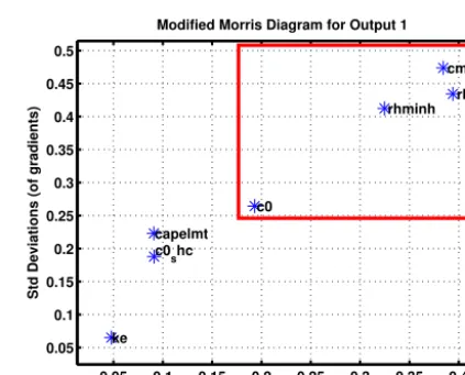
andσi are the sensitive parameters. The Morris method

re-sults are shown in Fig. 2.

0.05 0.1 0.15 0.2 0.25 0.3 0.35 0.4 0.05

0.1 0.15 0.2 0.25 0.3 0.35 0.4 0.45 0.5

c0

ke

rhminl

capelmt

rhminh

c0_shc

cmftau

Modified Means (of gradients)

Std Deviations (of gradients)

Modified Morris Diagram for Output 1

Figure 2. Scatter diagram showing the parameter sensitivity using

the Morris sensitivity analysis. Thexaxis stands for the main effect

sensitivity of a single parameter. Theyaxis stands for the

inter-active effect sensitivity among multi-parameters. In GAMIL2, c0, rhminl, rhminh, and cmftau have high sensitivity and ke, c0_shc, and capelmt have low sensitivity.

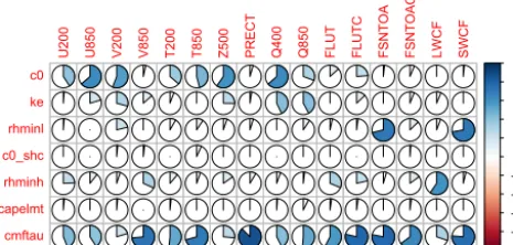
The parameter elimination step is critical for the final re-sult of model tuning. To validate the rere-sults obtained by the Morris method, we compare the results with a benchmark method (Sobol, 2001). Based on variance decomposition, the Sobol method requires more samples than the Morris method, leading to a higher computation cost. The variance of the model output can be decomposed as Eq. (7), where n is the number of parameters,Vi is the variance of theith

parameter, andVijis the variance of the interactive effect

be-tween theith andjth parameters, and so on. The total sensi-tivity effect of theith parameter can be presented as Eq. (8), whereV₋i is the total variance except for thexi parameter.

The Sobol results are shown in Fig. 3. The screened-out pa-rameters are the same as those of the Morris method.

V =

n X

i=1 Vi+

X

1≤i<j≤n

Vij+. . .+V1,2,...,n (7)

STi=1−

V₋i

(7)

-1 -0.8 -0.6 -0.4 -0.2 0 0.2 0.4 0.6 0.8 1

U200 U850 V2

00

V8

50

T200 T850 Z500 PR

EC

T

Q400 Q850 FLUT FLUTC FSN

T O A F SN T O AC LWCF SW C F c0 ke rhminl c0_shc rhminh capelmt cmftau

Figure 3. Sensitivity analysis results from the Sobol method. The

total sensitivity in Eq. (8) is denoted by the size of the color area. The total sensitivities of ke, c0_shc, and capelmt are less than 0.5 in terms of each variable.

4.3 Proper initial value selection for the downhill simplex method

The downhill simplex method is a local optimization algo-rithm and its convergence performance strongly depends on the quality of the initial values. We need to find the parame-ters with the smaller metrics around the final solution. More-over, we have to finish the searching as fast as possible with minimal overhead. For these two objectives, a hierarchical sampling strategy based on the single parameter perturbation (SPP) sample method is used. The SPP is similar to local sen-sitivity methods, in which only one parameter is perturbed at one time with other parameters fixed. The perturbation sam-ples are uniformly distributed across parametric space. First, the improvement index as defined in Eq. (3) of each param-eter sample is computed. The distance is defined as the dif-ference between the improvement indexes using two adja-cent samples, i.e., the model response measured by a certain percentage change of one parameter. We call this step the first-level sampling. The specific perturbation size for one parameter can be set based on user experience. In our im-plementation, the user needs to set the number of samples. For the first-level sampling, we can use a larger perturbation size to reduce computational cost. If the distance between two adjacent samples is greater than a predefined threshold, more SPP samples between the previous two adjacent ples are conducted, and this is called the second-level sam-pling. Finally,k+1 samples with the best improvement index value are chosen as the candidate initial values for the opti-mization method. With this hierarchical sampling strategy, we can determine the local parametric space for the final so-lution and can accelerate the convergence of the following downhill simplex method. This procedure is described in Al-gorithm 1. It is easy to implement and has lower overhead compared to other complex adaptive sampling methods.

6 Conclusions

An effective and efficient three-step method for GCM phys-ical parameter tuning is proposed. Compared with conven-tional methods, a parameter sensitivity analysis step and a proper initial value selection step are introduced before the low cost downhill simplex method. This effectively reduces the computational cost with an overall good performance. In addition, an automatic parameter calibration workflow is designed and implemented to enhance operational efficiency and support different uncertainty quantification analysis and calibration strategies. Evaluation of the method and work-flow by calibrating GAMIL2 model indicates the three-step method outperforms the two global optimization methods (PSO and DE) in both effectiveness and efficiency. A bet-ter trade-off between accuracy and computational cost is achieved compared with the two-step method and the orig-inal downhill simplex method. The optimal results of the three-step method demonstrate that most of the variables are improved compared with the control simulation, especially for the radiation related ones. The mechanism analysis is conducted to explain why these radiation related variables have an overall improvement. In future work, more analy-ses are needed to better understand the model behavior along with the physical parameter changes. The choosing of ap-propriate reference metrics and related observations are very important for the final tuned model performance. In future studies, we are going to use the more reliable and accurate observations, and add some constraint conditions for param-eters tuning to construct a more comprehensive and reliable

metrics.TS1

References

Adler, R. F., Huffman, G. J., Chang, A., Ferraro, R., Xie, P.-P., Janowiak, J., Rudolf, B., Schneider, U., Curtis, S., Bolvin, D., Gruber, A., Susskind, J., Arkin, P., and Nelkin, E.: The version-2 global precipitation climatology project (GPCP) monthly pre-cipitation analysis (1979–present), J. Hydrometeorol., 4, 1147– 1167, 2003.

Aksoy, A., Zhang, F., and Nielsen-Gammon, J. W.: Ensemble-based simultaneous state and parameter estimation with MM5, Geo-phys. Res. Lett., 33, L12801, doi:10.1029/2006GL026186, 2006. Allen, M. R., Stott, P. A., Mitchell, J. F., Schnur, R., and Del-worth, T. L.: Quantifying the uncertainty in forecasts of anthro-pogenic climate change, Nature, 407, 617–620, 2000.

Arulampalam, M., Maskell, S., Gordon, N., and Clapp, T.: A tutorial on particle filters for online nonlinear/non-Gaussian Bayesian tracking, Signal Processing, IEEE T., 50, 174–188, 2002. Bardenet, R., Brendel, M., Kégl, B., and Sebag, M.: Collaborative

hyperparameter tuning, in: Proceedings of the 30th International Conference on Machine Learning (ICML-13), 16–21 June 2013, Atlanta, Georgia, USA, 199–207, 2013.

Barkstrom, B. R.: The earth radiation budget experiment (ERBE), B. Am. Meteorol. Soc., 65, 1170–1185, 1984.

Algorithm 1 Preprocessing the initial values of Downhill

Simplex Algorithm.

1: //Single parameter perturbation sample(SPP) 2: N=number_of_parameters

3: sampling_sets={}

4: for each parameterPiofNparameters do

5: sampling_sets+=SPP(Pi_range, number_of_samples) 6: //refine sample in the sensitivity range if needed

7: if metrics of the the adjacent same parameter sampling points

>=sensitivity_threhold then

8: sampling_sets+=SPP(Pi_adjacent_parameter_range, re-fine_ number_of_factors)

9: end if

10: end for 11:

12: //Initial vertexes with parameters of theN₊1 minimum metrics

13: for each initialViofN+1 vertexes do

14: //get the parameters of theith minimum metrics 15: candidate_init_sets += min(i, sampling_sets) 16: end for

17:

18: //make sure the initial simplex geometry is well-conditioned 19: while one parameterkhave the same values in theN₊1 sets

do 20: j=1

21: //remove the parameter set with the worst metrics from can-didate_init_sets

22: remove_parameter_set(the parameter set with worse met-rics, candidate_init_sets)

23: //get the parameters of theN₊1₊jth minimum metrics 24: candidate_init_sets += min(N+1+j, sampling_sets) 25: j+ =1

26: end while

Beven, K. and Binley, A.: The future of distributed models: model calibration and uncertainty prediction, Hydrol. Process., 6, 279– 298, 1992.

Cameron, D., Beven, K. J., Tawn, J., Blazkova, S., and Naden, P.: Flood frequency estimation by continuous simulation for a gauged upland catchment (with uncertainty), J. Hydrol., 219, 169–187, 1999.

Campolongo, F., Cariboni, J., and Saltelli, A.: An effective screen-ing design for sensitivity analysis of large models, Environ. Mod-ell. Softw., 22, 1509–1518, 2007.

Chen, T.-Y., Wei, W.-J., and Tsai, J.-C.: Optimum design of head-stocks of precision lathes, Int. J. Mach. Tool. Manu., 39, 1961– 1977, 1999.

Eldred, M., Agarwal, H., Perez, V., Wojtkiewicz Jr., S., and Re-naud, J.: Investigation of reliability method formulations in DAKOTA/UQ, Struct. Infrastruct. E., 3, 199–213, 2007. Elkinton, C. N., Manwell, J. F., and McGowan, J. G.: Algorithms

for offshore wind farm layout optimization, Wind Engineering, 32, 67–84, 2008.

Evensen, G.: The ensemble Kalman filter: Theoretical formula-tion and practical implementaformula-tion, Ocean Dynam., 53, 343–367, 2003.

www.geosci-model-dev.net/8/1/2015/ Geosci. Model Dev., 8, 1–12, 2015 At the same time, inappropriate initial values may lead to ill-conditioned simplex geometry, which can be found in the model tuning process. One issue we meet is that some vertexes in the downhill simplex optimization may have the same values for one or more parameters. As a result, these parameters remain invariant during the optimization, and this may degrade the quality of the final solution as well as the convergence speed. A simplex checking is conducted to keep as many different values of parameters as possible during the process of looking for initial values. Well-conditioned sim-plex geometry will increase the parameter freedom for op-timization. In our implementation (Algorithm 1), the vertex leading to the ill-conditioned simplex is replaced by another parameter sample that gives another minimum improvement index value.

(8)

Table 4. The same as Table 3 but showing the comparison among the three downhill simplex methods.

Improvement index Nstep Nsize Core hours

Downhill_1_step 0.9585 80 1 14 400

Downhill_2_steps 0.9257 25+34 1 10 620

Downhill_3_steps 0.9099 80₊25₊50 1 27 900

Figure 4. Taylor diagram of the climate mean state of each output

variable from 2002 to 2004 of EXP and CNTL.

4.4 Evaluation of the proposed strategy

The effectiveness and efficiency of the three traditional al-gorithms are compared in Table 3. “Downhill_1_step” rep-resents the original downhill simplex method, which is one of the most widely used local optimization algorithms and has been successfully used in the Speedy model (Severi-jns and Hazeleger, 2005). PSO and DE are the most widely used global optimization algorithms and are easy to use. Al-though “Downhill_1_step” achieves slightly worse improve-ment compared to the two global optimization methods (Ta-ble 3), its computation cost is much less (only 20 and 28 % of DE and PSO, respectively).

Two extra steps are included before the original down-hill simplex method to overcome its limited effectiveness on model performance improvement. The “Downhill_2_steps” method includes an initial value pre-processing step before the downhill simplex method, and the “Downhill_3_steps” method further introduces another step to eliminate insen-sitive parameters for tuning by sensitivity analysis. The two steps bring in additional overhead, 80 samples for the param-eter sensitivity analysis with the Morris method, and 25 sam-ples for the initial value pre-processing. Tables 3 and 4 show that the proposed “Downhill_3_steps” achieves the best ef-fectiveness, improving the model’s overall performance by

Figure 5. Improvement indices over the global, tropical and mid–

high latitudes of the Northern and Southern Hemisphere (MLN and MLS) for each variable of the EXP simulation.

9 %. It overcomes the inherent ineffectiveness of the original downhill simplex method with a much lower computational cost than global methods.

5 Analysis of model optimal results

This section compares the default simulation and the tuned simulation by the three-step method, with a focus on the cloud and TOA radiation changes. Table 1 shows the values of the four pairs of sensitive parameters between the control (labeled as CNTL) and optimized (labeled as EXP) simula-tions. Significant change is found for c0, which represents the auto-conversion coefficient in the deep convection scheme, and rhminh, which represents the threshold relative humidity for high cloud appearance. The other two parameters have negligible change of the values before and after the tuning, and thus it is expected that their impacts on model perfor-mance will be accordingly small.

(9)

Figure 6. Pressure–latitude distributions of relative humidity and cloud fraction of EXP (a, d), CNTL (b, e), and EXP-CNTL (c, f).

three regions (tropics, SH middle and high latitudes and NH middle and high latitudes) are shown in Fig. 5. First, radia-tive fields and moisture are improved over all four areas. By contrast, wind and temperature field changes are more di-verse among different areas. For example, temperatures over the tropics become worse compared to the control run. There is an overall improvement at the SH middle and high lat-itudes for all variables except for the 200 hPa temperature. Winds and precipitation at the NH middle and high lati-tudes become slightly worse in the tuned simulation. Such changes are somewhat intriguing and we attempt to relate these changes to the two parameters significantly tuned.

With a reduced RH threshold for high cloud (from 0.78 in CNTL to 0.63 in EXP, Table 1), the stratiform

(10)

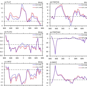
Figure 7. Meridional distributions of the annual mean difference between EXP/CNTL and observations of TOA outgoing long-wave

radia-tion (a), TOA clear-sky outgoing long-wave radiaradia-tion (b), TOA long-wave cloud forcing (c), TOA net short-wave flux (d), TOA clear-sky net short-wave flux (e), and TOA short-wave cloud forcing (f).

middle and high latitudes. On the contrary, low cloud below 800 hPa decreases by 1–2 % over the middle and high lat-itudes, with slightly decreased RH (Fig. 6) because of the negligible change of RH threshold for low cloud (Table 1). Overall, the combined effects of all relevant parameteriza-tions lead to the changes in atmospheric humidity and cloud fraction.

Changes in moisture and cloud fields impact radiative fields. With reference to ERBE, TOA outgoing long-wave radiation (OLR) is improved at the mid-latitudes for EXP, but it is degraded over the tropics (Fig. 7a). Compared with the CNTL, middle and high cloud significantly increase in the EXP (Fig. 6). Consequently, it enhances the blocking ef-fect on the long-wave upward flux at TOA (FLUT), reducing the FLUT in mid-latitudes of the Southern Hemisphere and Northern Hemisphere (Fig. 7a). Clear-sky OLR increases for the EXP and this is due to the drier upper troposphere in the EXP (Fig. 6). The decrease in the atmospheric water vapor reduces the greenhouse effect. Therefore, it emits more

out-going long-wave radiation and reduces the negative bias of clear-sky long-wave upward flux at TOA (FLUTC, Fig. 7b). Long-wave cloud forcing (LWCF) at the middle and high lat-itudes is improved due to the improvement in the FLUT in these areas (Fig. 7c), but improvement in the tropics is negli-gible due to the cancellation between the FLUT and FLUTC. Overall, the tuned simulation has a TOA radiation imbalance of 0.08 W m−2, which is better than that of the control run (0.8 W m−2).

(11)

6 Conclusions

An effective and efficient three-step method for GCM phys-ical parameter tuning is proposed. Compared with conven-tional methods, a parameter sensitivity analysis step and a proper initial value selection step are introduced before the low-cost downhill simplex method. This effectively reduces the computational cost with an overall good performance. In addition, an automatic parameter calibration workflow is designed and implemented to enhance operational efficiency and support different uncertainty quantification analysis and calibration strategies. Evaluation of the method and work-flow by calibrating the GAMIL2 model indicates that the three-step method outperforms the two global optimization methods (PSO and DE) in both effectiveness and efficiency. A better trade-off between accuracy and computational cost is achieved compared with the two-step method and the orig-inal downhill simplex method. The optimal results of the three-step method demonstrate that most of the variables are improved compared with the control simulation, especially for the radiation-related ones. The mechanism analysis is conducted to explain why these radiation-related variables have an overall improvement. In future work, more analy-ses are needed to better understand the model behavior along with the physical parameter changes. The choice of appro-priate reference metrics and related observations are very important for the final tuned model performance. In future studies, we are going to use the more reliable and accurate observations, and add some constraint conditions for param-eter tuning to construct a more comprehensive and reliable metrics.

Acknowledgements. The authors are grateful to the reviewers for valuable comments that have greatly improved the paper. This work is partially supported by the Ministry of Science and Technology of China under grant no. 2013CBA01805, the Information Technology Program of the Chinese Academy of Sciences under grant no. XXH12503-02-02-03, the China Special Fund for Meteorological Research in the Public Interest under grant no. GYHY201306062, and the Natural Science Foundation of China under grant nos. 91530103, 61361120098, and 51190101.

Edited by: R. Neale

References

Adler, R. F., Huffman, G. J., Chang, A., Ferraro, R., Xie, P.-P., Janowiak, J., Rudolf, B., Schneider, U., Curtis, S., Bolvin, D., Gruber, A., Susskind, J., Arkin, P., and Nelkin, E.: The version-2 global precipitation climatology project (GPCP) monthly pre-cipitation analysis (1979–present), J. Hydrometeorol., 4, 1147– 1167, 2003.

Aksoy, A., Zhang, F., and Nielsen-Gammon, J. W.: Ensemble-based simultaneous state and parameter estimation with MM5, Geo-phys. Res. Lett., 33, L12801, doi:10.1029/2006GL026186, 2006.

Allen, M. R., Stott, P. A., Mitchell, J. F., Schnur, R., and Del-worth, T. L.: Quantifying the uncertainty in forecasts of anthro-pogenic climate change, Nature, 407, 617–620, 2000.