www.geosci-model-dev.net/9/3321/2016/ doi:10.5194/gmd-9-3321-2016
© Author(s) 2016. CC Attribution 3.0 License.
A new stepwise carbon cycle data assimilation system using multiple
data streams to constrain the simulated land surface carbon cycle
Philippe Peylin1, Cédric Bacour2, Natasha MacBean1, Sébastien Leonard1, Peter Rayner1,3, Sylvain Kuppel1,4, Ernest Koffi1, Abdou Kane1, Fabienne Maignan1, Frédéric Chevallier1, Philippe Ciais1, and Pascal Prunet2
1Laboratoire des Sciences du Climat et de l’Environnement, UMR 8212 CEA-CNRS-UVSQ,
91191 Gif-sur-Yvette CEDEX, France
2Noveltis, Parc Technologique du Canal, 2 avenue de l’Europe, 31520 Ramonville-Saint-Agne, France 3University of Melbourne, 3010, Vic, Melbourne, Australia
4Grupo de Estudios Ambientales, IMASL-CONICET/Universidad Nacional de San Luis, San Luis, Argentina
Correspondence to:Philippe Peylin ([email protected])
Received: 14 January 2016 – Published in Geosci. Model Dev. Discuss.: 28 January 2016 Revised: 19 August 2016 – Accepted: 30 August 2016 – Published: 20 September 2016
Abstract.Large uncertainties in land surface models (LSMs) simulations still arise from inaccurate forcing, poor descrip-tion of land surface heterogeneity (soil and vegetadescrip-tion prop-erties), incorrect model parameter values and incomplete rep-resentation of biogeochemical processes. The recent increase in the number and type of carbon cycle-related observations, including both in situ and remote sensing measurements, has opened a new road to optimize model parameters via robust statistical model–data integration techniques, in or-der to reduce the uncertainties of simulated carbon fluxes and stocks. In this study we present a carbon cycle data as-similation system that assimilates three major data streams, namely the Moderate Resolution Imaging Spectroradiometer (MODIS)-Normalized Difference Vegetation Index (NDVI) observations of vegetation activity, net ecosystem exchange (NEE) and latent heat (LE) flux measurements at more than 70 sites (FLUXNET), as well as atmospheric CO2
concen-trations at 53 surface stations, in order to optimize the main parameters (around 180 parameters in total) of the Organiz-ing Carbon and Hydrology in Dynamics Ecosystems (OR-CHIDEE) LSM (version 1.9.5 used for the Coupled Model Intercomparison Project Phase 5 (CMIP5) simulations). The system relies on a stepwise approach that assimilates each data stream in turn, propagating the information gained on the parameters from one step to the next.
Overall, the ORCHIDEE model is able to achieve a con-sistent fit to all three data streams, which suggests that cur-rent LSMs have reached the level of development to
assim-ilate these observations. The assimilation of MODIS-NDVI (step 1) reduced the growing season length in ORCHIDEE for temperate and boreal ecosystems, thus decreasing the global mean annual gross primary production (GPP). Us-ing FLUXNET data (step 2) led to large improvements in the seasonal cycle of the NEE and LE fluxes for all ecosys-tems (i.e., increased amplitude for temperate ecosysecosys-tems). The assimilation of atmospheric CO2, using the general
cir-culation model (GCM) of the Laboratoire de Météorologie Dynamique (LMDz; step 3), provides an overall constraint (i.e., constraint on large-scale net CO2fluxes), resulting in
an improvement of the fit to the observed atmospheric CO2
1 Introduction
Atmospheric CO2 concentrations have increased at an
un-precedented rate over the last few decades, predominantly due to anthropogenic fossil fuel and cement emissions, as well as land use and land cover change (LULCC). The oceans and the terrestrial biosphere have absorbed CO2, removing
on average 50 % of anthropogenic emissions from the at-mosphere. However, knowledge about the exact location of sources and sinks of carbon (C) and the driving mechanisms is still lacking. Land surface models (LSMs) can be used to improve our understanding of the spatiotemporal patterns of sources and sinks, as well as for attributing changes due to CO2, climate variability and other environmental drivers.
However, the spread in the model predictions of terrestrial net C (carbon) exchange currently has the same order of magni-tude as the uncertainty of the terrestrial C budget estimated as the residual of the other carbon cycle components (Le Quéré et al., 2015). In addition to uncertainties in the mean global annual terrestrial C budget and its trend over time (Sitch et al., 2015), there remain strong discrepancies between LSMs in their predictions of regional budgets (Canadell et al., 2013) at seasonal and interannual timescales and in their sensitivity to climate and atmospheric CO2forcing (Piao et al., 2013).
Uncertainties in model simulations arise from inaccurate forcing, incorrect model parameter values and/or an inade-quate or incomplete representation of biogeochemical pro-cesses in the model (for example the impact of nutrient limitation on C fluxes, or C release related to permafrost thawing). Arguably the best way to improve model predic-tions is to confront simulapredic-tions with multiple sources of data within an appropriate and rigorous framework (Prentice et al., 2015). In the last 2 decades significant efforts by the site and satellite observation communities have resulted in a large increase in the number and type of C cycle-related observa-tions. These data contain some information at various spatial and temporal scales and should be combined together to ro-bustly address different aspects of the models. One way in which these data can be used to better quantify and reduce model uncertainty is by optimizing or calibrating the model parameters via robust statistical model–data fusion (or data assimilation – DA) techniques. In particular a Bayesian in-ference framework allows us to update our prior knowledge of the parameters based on new information contained in the observations.
There is a long history of using DA techniques for pa-rameter optimization, particularly in geophysics (Tarantola, 1987), but the initial studies in the field of global terres-trial C cycle data assimilation started with the initial study of Fung et al. (1987) and a pioneering work by Knorr and Heimann (1995), who used atmospheric CO2
concentra-tion to constrain the Simple Diagnostic Biosphere Model (SDBM). Later, Kaminski et al. (2002) constrain the sea-sonal cycle of SDBM with the same data stream. This effort was continued by the original Carbon Cycle Data
Assimi-lation System (CCDAS) described in Rayner et al. (2005) and Kaminski et al. (2012), which used both atmospheric CO2 and satellite-derived Fraction of Absorbed
Photosyn-thetic Radiation (FAPAR) data to optimize vegetation pro-ductivity by adjusting the C cycle-related parameters of the Biosphere Energy-Transfer Hydrology (BETHY) model (see a review in Kaminski et al., 2013). Note that although Rayner et al. (2005) did use, in addition to atmospheric CO2data,
soil moisture and radiation fields from an earlier assimilation from a simpler model version, no parameters were passed between the two assimilations and very little comment was made on the consistency between the two assimilations, an important issue that will be central to this paper. Meanwhile substantial efforts have been put into the use of local eddy covariance flux tower measurements of net exchange of CO2
and latent and sensible heat fluxes to optimize photosyn-thesis, respiration and energy-related parameters of terres-trial ecosystem models, both at individual sites (e.g., Wang et al., 2001, 2007; Williams et al., 2005; Braswell et al., 2005; Knorr and Kattge, 2005; Moore et al., 2008; Ricciuto et al., 2008) and more recently using multiple sites together (hereafter multiple sites) from the global FLUXNET network (e.g., Groenendijk et al., 2011; Kuppel et al., 2012, 2014; Al-ton, 2013; Xiao et al., 2014). Increasingly the focus in carbon cycle data assimilation is moving towards using multiple dif-ferent data streams as independent constraints, with the aim of bringing more information at different spatial and tempo-ral scales and constraining sevetempo-ral processes at once in order to reduce the likelihood of model equifinality (where multi-ple sets of parameters achieve the same reduction in model– data misfit). Recent examples include the combination of in situ eddy covariance flux observations and ground-based in-formation on vegetation structure and C stocks (Richardson et al., 2010; Ricciuto et al., 2011; Keenan et al., 2012, 2013; Thum et al., 2016), or in situ flux data and satellite FAPAR (Kato et al., 2013; Zobitz et al., 2014; Bacour et al., 2015) or atmospheric CO2and biomass data using a simple biosphere
model (Saito et al., 2014). This is a non-trivial task however, especially when optimizing a complex LSM (see MacBean et al., 2016), which has many parameters acting from local to global scales.
(and whether the system is linear or not). In complex prob-lems such as these, one cannot carry or even describe the full structure of the relevant probability densities, so which ap-proach will work best in each case is unclear. In particular, technical difficulties associated with the different number of observations for each data stream and the characterization of error correlations between them, in addition to compu-tational constraints to run global LSMs, might result in the preference for a stepwise assimilation framework. Addition-ally, it may be more straightforward, to expose a restricted set of parameters (following a global sensitivity analysis) to each observation type in a stepwise approach to ensure that each data stream constrains only the most relevant parts of the model. This reduces biases from other poorly represented processes caused by inadequate model structure. Note finally that more complex approaches based on random generation of parameter sets, such as the multi-objective approach us-ing the Pareto rankus-ing of several cost functions (e.g., Yapo et al., 1998), are not yet affordable for global LSMs from a computational point of view. For these reasons we follow the stepwise approach in this paper.
We present the first global-scale CCDAS that assimilates three of the main global data streams that have been used to date to understand the terrestrial carbon cycle – atmospheric CO2 concentration, satellite-derived information of
vegeta-tion greenness (from the Moderate Resoluvegeta-tion Imaging Spec-troradiometer, MODIS, instrument) and multi-site eddy co-variance net CO2and latent heat flux measurements (from
FLUXNET) – to optimize the parameters of the Organiz-ing Carbon and Hydrology in Dynamics Ecosystems (OR-CHIDEE) process-based LSM (Krinner et al., 2005). This study is the first (to our knowledge) to assimilate these three major data streams in a process-based LSM used as the land component of an Earth system model (ESM), the French In-stitut Pierre Simon Laplace ESM. Two contemporary stud-ies also optimize the parameters of the land component of an ESM; however, Raoult et al. (2016) only used FluxNet observations to optimize the parameters of the Joint UK Land Environment Simulator (JULES) model, while Schür-mann et al. (2016) only assimilate two data streams (FA-PAR and CO2) in the JSBACH (Jena Scheme for
Biosphere-Atmosphere Coupling in Hamburg) model at coarse resolu-tion (10◦×10◦). Note finally that the level of complexity of the ecosystem model (and the spatial resolution) is part of the problem: achieving an optimization with a given model does not guarantee that the framework would work with a more complex or different one.
In this context, the main questions that we aim to answer in this paper are as follows:
i. How and to which extend the optimization of the OR-CHIDEE model allows one to fit the three data streams that are considered?
ii. Does the stepwise optimization result in a degradation of the fit to other data streams used in the previous steps?
iii. What are the main changes in the optimized parameters when using sequentially these three data streams in a global CCDAS and which processes are constrained? iv. What are the improvements for the land C cycle in
terms of net/gross fluxes and stocks as a result of multi-data stream optimization? What preliminary perspec-tives can we draw that may help us in improving model predictions of trends, variability and the location of ter-restrial C sources and sinks?
Following these objectives, the paper first describes the new ORCHIDEE-CCDAS including the concept, the observa-tions, the models and the optimization approach. We then present the results, including the fit to the data, consistency checks (question i, above) as well as the mean global and re-gional C cycle budget for the period 2000–2009. The last sec-tion discusses issues and perspectives associated with these results.
2 Methods
2.1 ORCHIDEE-CCDAS concept
We have designed a CCDAS around the ORCHIDEE land surface model (ORCHIDEE-CCDAS, later also referred to as ORCHIDAS for simplicity) that combines a state-of-the-art description of the driving biogeochemical processes within the model with multiple observational constraints in a robust statistical framework, in order to improve the simulation of land carbon fluxes and stocks. The system allows us to re-trieve the best estimate, given the observations and prior in-formation, of selected parameters (see Sect. 2.3.3) as well as to evaluate their uncertainty. It relies on a stepwise assim-ilation of a comprehensive set of three C cycle-related ob-servations that are representative of small (100 m) to large (continental) scales (see Sect. 2.2):
– step 1: satellite measurements of vegetation activ-ity using the Normalized Difference Vegetation Index (NDVI) from the MODIS instrument over the 2000-2008 period for a randomly selected set of sites for bo-real and temperate deciduous vegetation types;
– step 2: in situ eddy covariance net CO2and water (latent
heat) flux measurements from the FLUXNET database for a large set of sites, spanning seven different vegeta-tion types;
– step 3: in situ monthly atmospheric surface CO2
Carbon data assimila.on system
Meteo. data prior param.
calibration
Optimized model parameters
è Carbon fluxes & pools
(values & uncertainties) Satellite
data (NDVI)
Atmos. conc. (CO2)
Fossil fuel & biomass bur
fluxes
Flux tower (NEE, LE)
Assimilation data Forcing data
Ocean fluxes
Validation data
CO2 vertical
Profiles Forest & soil C stock change
Satellite biomass data
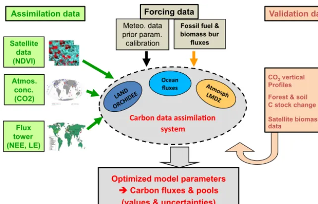
Figure 1.Schematic of the ORCHIDEE Carbon Cycle Data Assimilation System (ORCHIDAS).
The system relies on two models:
– the ORCHIDEE global LSM, whose main C cycle pa-rameters are optimized (see Sect. 2.3);
– the GCM of the Laboratoire de Météorologie Dy-namique, LMDz (see Sect. 2.3), to relate the surface carbon fluxes to atmospheric CO2concentrations.
The framework combines the different observational data streams within ORCHIDAS in order to optimize selected model parameters using a variational data assimilation sys-tem, described in Sect. 2.4. Figure 1 illustrates the struc-ture of the CCDAS and the different components that are involved. Such a framework distinguishes (i) the assimi-lated observations, (ii) an ensemble of forcing and input data streams, (iii) the models and optimization framework, as well as (iv) an evaluation step, where independent data sets are compared to the optimized model stocks and fluxes. As ex-plained in the introduction, a major feature of the current sys-tem is the stepwise approach, in which all data streams are assimilated sequentially (i.e., one after the other). The infor-mation retrieved at a given step (retrieved optimal parameter values and associated uncertainty) is propagated to the next step (see Fig. 2 and Sect. 2.4). Note that for simplicity we did not propagate the error correlations in this first implementa-tion of the system, a simplificaimplementa-tion that appeared sufficient (see the consistency analysis in Sect. 3.2); Sect. 4 also dis-cusses the potential impact of this simplification.
At each step, the parameter optimization relies on a Bayesian framework that explicitly minimizes the difference between the simulated and observed quantities in addition to minimizing the difference between the optimized model pa-rameters and “a priori” values (see Sect. 2.4.2). The depen-dence of the simulated quantities on the optimized variables
ORCH ORCH
Satellite NDVI
Fluxes NEE, LE
atm. CO2 x0
B0
x3CO2 B3CO2 x2flux
B2ux x1sat
B1sat
Optimized fluxes & stocks ORCH LMDz
Figure 2. Illustration of the stepwise data assimilation ap-proach used for the assimilation of multiple data streams in the ORCHIDEE-CCDAS. The list of parameters for each step is sum-marized in Table 1.
is nonlinear, which thus necessitates the use of an iterative algorithm. Note that all components of the surface C bud-get need also to be included in the ORCHIDAS, particularly when using atmospheric CO2measurements, which requires
the atmospheric transport model to be prescribed with fos-sil fuel emissions, CO2fluxes associated with biomass
burn-ing and ocean CO2 fluxes (see Sect. 2.5) in addition to net
ecosystem exchange (NEE) from ORCHIDEE. 2.2 Assimilated observations
2.2.1 MODIS-NDVI
to the 0.72◦spatial resolution of the ERA-Interim meteoro-logical fields that are used to force ORCHIDEE, (ii) inter-polated to a daily time series (for practical implementation) and (iii) checked for quality (see MacBean et al., 2015 for details). If there is a gap in the observations of more than 15 days, no interpolation is done (i.e., no data during the gap are assimilated). Figure 3 displays the location of the sites that were selected (see Sect. 2.4.1).
2.2.2 Eddy covariance flux data
Eddy covariance flux measurements of net surface CO2flux
– hereafter referred to as NEE and latent heat (LE) flux – from 78 observation sites of a network of regional networks (FLUXNET; see Fig. 3) are used to constrain ecosystem physiology and fast C-related processes at daily to seasonal timescales in ORCHIDEE in the second step. We use quality-checked and gap-filled data from a global synthesis called the La Thuile data set (Papale, 2006). In order to avoid deal-ing with the large error correlations in the half-hourly data (see Lasslop et al., 2008), daily mean values of NEE and LE are used in the ORCHIDAS. Days with less than 80 % of the half-hourly data are left out of the assimilation. The selection of the sites and the data processing (gap-filling, correction for energy balance closure) are detailed in Kuppel et al. (2014). Note that uncertainties due to incomplete sampling of the di-urnal cycle are likely very small (less than 5 %) as the error in the gap-filling procedure is usually less than 20 % (Lasslop et al., 2008).
2.2.3 Atmospheric CO2concentrations
Atmospheric CO2 concentration measurements were taken
from an ensemble of selected surface stations around the world (Fig. 3). The spatial concentration gradients relate to the integral of the fluxes over large areas and thus al-low the optimization of large-scale global patterns of car-bon fluxes. These data were taken from the NOAA Earth System Laboratory (ESRL) GLOBALVIEW-CO2 collabo-rative product (GLOBALVIEW-CO2, 2013) and averaged to monthly means. We assimilated the monthly values for 53 sites for the 2002–2004 period inclusive in the last step of the assimilation system. Such a restricted period (3 years only) was chosen for practical reasons (computing resources) while constructing the ORCHIDAS system. The station lo-cations, indicated in Fig. 3, favor the background conditions; i.e., the surrounding air masses are only weakly influenced by local continental sources, such as power plants. The choice of monthly mean is related to the use of pre-calculated trans-port fields with LMDz (see Sect. 2.3.2). We also used addi-tional sites to evaluate the result of the optimization (loca-tions indicated in Fig. 3): this included 17 continental sites that are more directly influenced by local fluxes potentially not well captured at the considered LMDz spatial resolu-tion and 7 sites from Pacific Ocean cruises that were not
in-Figure 3.Location of the different observations used for each data stream assimilated in the system: MODIS-NDVI measurements, FLUXNET sites with NEE and LE measurements and atmospheric CO2stations (both the sites that are assimilated and the sites used for the validation).
cluded in the optimization in order not to overweight that the data contribution from that particular region. Note that we did not considered free troposphere aircraft data or column integrated measurements (TCCON sites) in this evaluation, although they are less sensitive to biases in the planetary boundary layer representation, given that (i) we are using pre-calculated transport fields previously computed at sur-face stations only and (ii) a few scarce free tropospheric data sets will not bring much more information to the additional surface stations.
2.3 Models and optimized parameters 2.3.1 ORCHIDEE land surface model
In this study we use the ORCHIDEE process-oriented land surface model (Krinner et al., 2005), which computes wa-ter, carbon and energy balances at the land surface on a half-hourly time step, using a mechanistic description of the phys-ical and biogeochemphys-ical processes (see, http://labex.ipsl.fr/ orchidee/). The model describes the exchange of carbon and water at the leaf level, the allocation of carbon within plant compartments (leaves, roots, heartwood and sapwood), the autotrophic respiration, the production of litter, the plant mortality and the degradation of soil organic matter (CEN-TURY model; Parton et al., 1988). The hydrological pro-cesses for the soil reservoir rely on a double bucket scheme (Ducoudré et al., 1993). The link between the water and car-bon modules is via photosynthesis, which is based on the leaf-scale equations of Farquhar et al. (1980) for C3plants,
and Collatz et al. (1992) for C4 plants, that are then integrated over the canopy by assuming an exponential attenuation of light. The FAPAR by each layer of the canopy is calculated from the leaf area index (LAI) following a Beer–Lambert ex-tinction law (Bacour et al., 2015).
(including bare soil) that can co-exist in each grid cell. Ex-cept for the phenology (see a recent description in MacBean et al., 2015), the equations governing the different processes are generic, but with specific parameter values for each PFT. Detailed descriptions of model equations can be found in nu-merous publications (see for instance Krinner et al., 2005). ORCHIDEE can be run at either global scale on a grid, or at site level using point-scale surface meteorological forc-ing variables. It is the land surface component of the Insti-tut Pierre Simon Laplace (IPSL) Earth system model, and the version that we used corresponds to Coupled Model In-tercomparison Project Phase 5 (CMIP5) simulations in the IPCC 5th Assessment Report (Dufresne et al., 2013). How-ever, in this study the model is run offline using the ERA-Interim 3-hourly near-surface meteorological forcing fields (Dee et al., 2011) aggregated at the spatial resolution of the atmospheric transport model for the global simulations (2.5◦×3.75◦; see Sect. 2.3.2). However, when we assimi-late in situ flux data in the second step, we force the model with the gap-filled half-hourly meteorological data measured at each site. The global PFT map was derived from the high-resolution IGBP AVHRR land data set (Vérant et al., 2004). The carbon pools are brought to equilibrium (spin-up proce-dure) for both site and global-scale simulations by cycling the available meteorological forcing over several millennia, to ensure that the long-term net carbon flux is close to zero. For the global simulation in the third step, we spun-up the model recycling the 1989–1998 meteorology and then used a transient simulation from 1990 to 2001 with changing cli-mate (ERA-Interim) and increasing CO2, before starting the
optimization with atmospheric data over 2002–2004. For the site simulations (i.e., the assimilation of flux data), we re-cycled the available in situ meteorological forcing to spin-up the model, with present-day CO2. Note that the use of
soil carbon data, such as from the Harmonized World Soil Database (as well as aboveground biomass data), to initial-ize the model is not straightforward and represents a chal-lenge to keep the internal model consistency, given that the three soil carbon reservoirs of the CENTURY model are in balance with all components of the model, in particular the input through the different litter pools. Computational and scientific issues to avoid a spin-up approach are still under investigation with ORCHIDEE (see discussion section). 2.3.2 LMDz model
The transport model used in this study is version 3 of the GCM, LMDz (Hourdin and Armengaud, 1999) with a hor-izontal resolution of 3.75◦ (longitude)×2.5◦(latitude) and 19 sigma-pressure layers up to 3 hPa. The calculated winds (u andv) are relaxed to the European Centre for Medium-Range Weather Forecasts (ECMWF) reanalysis, ERA-40, meteorological data (Uppala et al., 2005) with a relaxation time of 2.5 h (guiding) in order to realistically account for large-scale advection (Hourdin et al., 2006). Deep convection
is parameterized according to the scheme of Tiedtke (1989) and the turbulent mixing in the planetary boundary layer is based on a local second-order closure formalism. The LMDz GCM model has been widely used to model climate (IPCC, 2007) and its derived transport model has been used for the simulation of chemistry of gas and particles and greenhouse gases distributions (Hauglustaine et al., 2004; Folberth et al., 2005; Bousquet et al., 2005; Rivier et al., 2006). For this study, we used pre-calculated transport fields, as described in Peylin et al. (2005), that correspond to the sensitivity of concentration at each atmospheric site and each month to the surface flux of each model grid cell for each day (often called influence functions). The sensitivities (using interan-nual winds) were calculated with the “retro-transport” for-mulation implemented in the LMDz transport model (Hour-din et al., 2006). This approach decreases the computing time of the optimization compared to the use of the full forward LMDz model at each iteration, as the transport is replaced by a matrix multiplication with the vector of surface fluxes. Note that the initial 3-D state of the atmospheric concentra-tions was defined from Chevallier et al. (2010).
2.3.3 Parameters optimized
The optimized parameters are described in Table 1, and their prior values, uncertainty and range are given in Table 2. In the most recent studies using ORCHIDAS at site scales, a large set of ORCHIDEE parameters has been optimized (Kuppel et al., 2014; Santaren et al., 2014; Bacour et al., 2015). In this study a smaller set was chosen, based on a Morris sen-sitivity analysis (Morris, 1991; results not shown) that deter-mines the sensitivity of the NEE and LE to all model param-eters at various FLUXNET sites (for each PFT), in order to reduce the computational cost of the global optimization in step 3 (see Sect. 2.5). We considered nine PFT-dependent and four “global” (i.e., non-PFT-dependent) parameters that con-trol mostly the fast carbon processes (diurnal to seasonal). In addition, we introduced a new parameter,KsoilC, to scale the
initial values (after spin-up) of the modeled slow and passive soil carbon pools, in order to take account of all the historical effects not accounted for in the model that would result in a disequilibrium of these pools in reality. For the site-specific optimizations with FLUXNET data, we have oneKsoilC,site
parameter per site. For the global-scale optimization step, we used 30KsoilC,regparameters corresponding to 30 regions
potentially coherent for land use and land management his-tory as well as ecosystem and edaphic properties (see Fig. A2 in the Appendix). The initial soil carbon pools of all pixels within each region were thus scaled by the same value. The prior value for allKsoilCparameters was set to one; i.e., the
default state of soil carbon pools is assumed to be in equilib-rium.
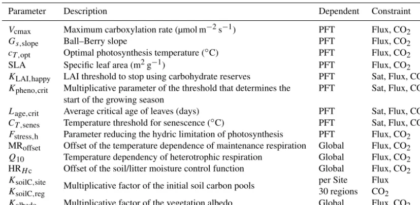
Table 1.Parameters description, generality (PFT dependent, global, specific to FLUXNET sites or for a set of regions) and data stream(s) that were used to constrain them.
Parameter Description Dependent Constraint
Vcmax Maximum carboxylation rate (µmol m−2s−1) PFT Flux, CO2
Gs,slope Ball–Berry slope PFT Flux, CO2
cT ,opt Optimal photosynthesis temperature (◦C) PFT Flux, CO2
SLA Specific leaf area (m2g−1) PFT Flux, CO2
KLAI,happy LAI threshold to stop using carbohydrate reserves PFT Sat, Flux, CO2
Kpheno,crit Multiplicative parameter of the threshold that determines the PFT Sat, Flux, CO2 start of the growing season
Lage,crit Average critical age of leaves (days) PFT Sat, Flux, CO2
CT ,senes Temperature threshold for senescence (◦C) PFT Sat, Flux, CO2
Fstress,h Parameter reducing the hydric limitation of photosynthesis PFT Flux, CO2 MRoffset Offset of the temperature dependence of maintenance respiration Global Flux, CO2
Q10 Temperature dependency of heterotrophic respiration Global Flux, CO2
HRHc Offset of the soil/litter moisture control function Global Flux, CO2
KsoilC,site Multiplicative factor of the initial soil carbon pools per Site Flux
KsoilC,reg 30 regions CO2
Kalbedo Multiplicative factor of the vegetation albedo Global Flux, CO2
pool scalars (one for each FLUXNET site) and 30 regional soil C pool scalars for the global simulations – a total of 184 parameters (16, 134 and 86 in step 1, 2 and 3, respec-tively). Note that the soil C pool multipliers at the FLUXNET sites are independent from the regional C pool multipliers, as the history of soil carbon over large eco-regions of sev-eral millions square kilometers is rather heterogeneous (as it is mainly related to previous land use changes) and, most likely, the FLUXNET sites are not representative of larger regions in terms of the soil carbon disequilibrium. The prior standard deviation for each parameter is equal to 40 % of the parameter range (lower and higher boundaries) prescribed for each parameter following Kuppel et al. (2012). The pa-rameter ranges were specified following expert judgment of their meaning in the ORCHIDEE equations and based on lit-erature reviews or databases (such as the global database of plant traits, TRY; Kattge et al., 2011).
2.4 System description: a stepwise approach 2.4.1 Stepwise assimilation of three data streams The ORCHIDAS system relies on a stepwise assimilation of the three data streams described in Sect. 2.2. Figure 2 illus-trates the flow of information in this sequential approach:
Step 1 – assimilation of MODIS-NDVI: four parame-ters related to the seasonal cycle of the vegetation (phenol-ogy) are optimized for the temperate and boreal deciduous PFTs (TeBD: temperate broadleaf deciduous, BoND: boreal needleleaf deciduous, BoBD: boreal broadleaf deciduous and NC3; see caption of Table 2). These four deciduous PFTs
alone are considered in step 1 in this ORCHIDAS version because the tropical deciduous phenology modules in OR-CHIDEE require further modifications to improve the
func-tions that control leaf growth and fall in response to water availability (MacBean et al., 2015). Evergreen PFTs were also not considered, as there are no phenology modules re-lated to these PFTs in the model. The procedure is similar to that described in detail in MacBean et al. (2015) and there-fore only briefly recalled here. A simple linear relationship between the modeled FAPAR and MODIS-NDVI observa-tions is assumed, based on studies such as Knyazikhin et al. (1998). Given that considerable discrepancies exist be-tween so-called “high-level” satellite products such as LAI or FAPAR when considering their magnitude (D’Odorico et al., 2014), we thus only use the temporal information in the NDVI observations and normalized both the model FAPAR output and the NDVI observations to their 5th and 95th per-centiles (following Bacour et al., 2015, and MacBean et al., 2015). Note that assimilating raw FAPAR data with the OR-CHIDEE model led to the degradation of the NEE with the estimation of spurious parameter values (Bacour et al., 2015). The model was run for 15 randomly selected grid cells for each of the four PFTs using the ERA-Interim meteorologi-cal forcing. Only grid cells that included vegetation fraction of greater than 60 % for the PFT optimized were considered. We selected a set of grid points instead of the whole grid to substantially decrease the computing time; but the remaining points are used for the evaluation of the optimized model. The 15 sites for each PFT were included in one optimization for each PFT following a multi-site approach, in which all observations are used simultaneously to optimize the model parameters. The optimized parameters are described in Ta-ble 1. They correspond to a scalar on the growing degree days (GDD) threshold for the start of the vegetation (Kpheno,crit), a
for the onset of leaf senescence (CTsenes) and the critical age
for leaves (Lagecrit).
Step 2 – assimilation of FLUXNET data: mean daily NEE and LE flux measurements for 78 sites, including up to 10 years worth of data for each site, are used to optimize a set of model parameters controlling the fast carbon and wa-ter processes (photosynthesis, respiration, phenology; see Ta-ble 1). The site selection and the choice of a daily time step are described in more details in Kuppel et al. (2014). These sites cover seven of the PFTs in ORCHIDEE (see Table 2). The posterior parameter values of the four phenology param-eters derived in step 1, and their associated uncertainties, are input as prior information in step 2. For the additional param-eters, the default ORCHIDEE values are used for the prior and the uncertainties are set as described in Sect. 2.3.3. A multi-site optimization is performed for each PFT indepen-dently as in step 1. Global parameters, i.e., those that are not PFT-dependent, were optimized for each PFT and the mean across all PFTs was then calculated to define the prior pa-rameter vector in step 3 of the assimilation with atmospheric CO2data (at global scale). Such an approach was chosen to
allow us to optimize all PFTs in parallel and therefore to sim-plify the assimilation process.
Step 3 – assimilation of atmospheric CO2 concen-trations: we use monthly mean CO2 concentrations from
53 surface stations over 3 years (2002–2004) to provide a large-scale constraint to the land surface fluxes (i.e., to match the global CO2growth rate, mean seasonal cycle and its
lat-itudinal variation, as well as the spatial gradients between stations). We use the LMDz atmospheric transport model (see Sect. 2.3.2) to assimilate these observations. The set of parameters optimized in step 2 are included in step 3, ex-cept for the albedo scaling parameter (Kalbedo,veg), as the net
carbon fluxes are only weakly sensitive to that parameter. We used the posterior parameter distributions from step 2 (parameter optimal values and associated uncertainties) as prior information for step 3, and expanded the parameter vec-tor to include the 30KsoilC parameters that scale the initial
soil carbon pools for large “spatially coherent regions” (see Sect. 2.1.2 and Fig. A2). The air–sea fluxes and fossil fuel and biomass burning emissions are also accounted for (but not optimized) in this final step, in order to close the global carbon budget within the atmospheric transport model (see Sect. 2.5).
2.4.2 Optimization procedure (for all steps)
In each step the statistically optimal parameter values are de-rived with an optimization procedure following the principle of the 4-D variational assimilation systems (developed for numerical weather prediction), using a tangent linear opera-tor (and finite differences for a few parameters, Bacour et al., 2015). Assuming that the errors associated with the parame-ters, the observations and the model outputs follow Gaussian distributions, the optimal parameter set corresponds to the
minimum of a cost function,J (x), that measures the mis-match between (i) the observations (y) and the corresponding model outputs,H (x), (whereHis the model operator), and (ii) the a priori (xb) and optimized parameters (x), weighted by their error covariance matrices (Tarantola, 1987; chap. 4):
J (x)=1
2
h
(H (x)−y)TR−1(H (x)−y)
+(x−xb)TB−1(x−xb)
i
. (1)
Rrepresents the error variance/covariance matrix associated with the observations andBthe parameter prior error vari-ance/covariance matrix. At each step a different cost func-tion is defined with the observafunc-tions and parameters related to that step (see Fig. 2).Rincludes the errors on the measure-ments, the model structure and the meteorological forcing. Model errors are rather difficult to assess and may be much larger than the measurement error itself. Therefore we chose to focus on the structural error and defined the variances inR as the mean squared difference between the prior model and the observations for both steps 1 and 2 (see Kuppel et al., 2013). For simplicity we assumed that the observation error covariances were independent between the different observa-tions and therefore we keptRdiagonal (off-diagonal terms set to zero), given the rapid decline of the model error auto-correlation beyond 1 day (Kuppel et al., 2013). For step 3 we used a different approach, given the large bias in the model a priori concentrations, and therefore followed the methodol-ogy of Peylin et al. (2005) based on the observed and mod-eled temporal concentration variability at each site. Overall, data uncertainties in the optimization procedure are between 0.1 and 0.45 for NDVI (step 1), around 3–6 mg C m−2d−1for
daily NEE, and 15–30 Wm−2for daily LE (step 2) and
be-tween 0.1 ppm at remote oceanic stations and 4 ppm at con-tinental sites (step 3).
The determination of the optimal parameter vector that minimizes J (x) is performed by successive calls to a “gradient-descent” minimization algorithm L-BFGS-B (Byrd et al., 1995), which is specifically dedicated to solv-ing large nonlinear optimization problems that are subject to simple bounds on the parameter values. In order to find the minimum ofJ (x), the algorithm requires the gradient ofJ (x)(Jacobian) with respect to the ORCHIDEE param-eters. L-BFGS-B explores each parameter space simultane-ously along the gradient of the cost function, and uses an approximation of the Hessian (second derivative) ofJ (x), which is updated at each iteration, to define the size of the step at each iteration.
to the model phenology for which the threshold functions prevent the use of a linear approximation. A finite difference approach was used for these parameters in order to define a mean derivative at any point; we also checked that no spu-rious oscillations occurred for these parameters during the minimization iterations.
For step 3, the model “H” corresponds to the composition of the land surface model with the transport model:H=T
oS(see Kaminski et al., 2002 for details), withT represent-ing the LMDz transport model. T is a linear operator for a non-reactive species: T (S(x))=T×S(x), withTa matrix representation of the transport operator. It corresponds to the sensitivity of CO2 concentrations at each site and for each
month to the daily surface flux of each model grid cell. It is then combined with the ORCHIDEE surface fluxes (S(x)) through a matrix multiplication to derive H (x).Thas been pre-calculated for all atmospheric stations in order to save computing time during the iterative optimization process (see Sect. 2.3.2). For simplicity we use monthly mean values for both the fluxesS(x)and the transport sensitivities (T) in the computation of the gradients dJ (x)/dx.
For improved minimization efficiency, the inversion is preconditioned (following Chevallier et al., 2005), which means that L-BFGS-B is fed with the control variablex0= B−1/2(x−xb), rather than withx, as this homogenizes the range of variation of the optimized parameters.
2.4.3 Error estimation
The posterior parameter error covariance matrix, A, can be approximated to the inverse Hessian of the cost function, us-ing the linearity assumption at the minimum ofJ (x). It can be derived with the Jacobian of the model at the end of the minimization (i.e., the last iteration),H∞, following Taran-tola (1987):
A=hHT∞×R
−1×H∞+B−1i−1. (2)
Note that for step 3,H∞=T×S∞, whereS∞is the Jaco-bian of the ORCHIDEE model at the last iteration. The pos-terior parameter error covariance,A, can then be propagated into the model state variable space (e.g., carbon fluxes and stocks),Avar, given the following matrix product (only used
for the global fluxes in step 3):
Avar=S∞×A×ST∞. (3)
The square root of the diagonal elements ofAvarcorresponds
to the standard deviation,σ, of carbon fluxes/stocks for each grid cell. In order to evaluate the knowledge improvement brought by the assimilation, the uncertainty reduction be-tween the prior (σprior) and posterior (σpost) is determined as
1−(σpost/σprior).
2.4.4 Additional processing steps
In order to analyze the fit to the atmospheric CO2
concen-trations in terms of the trend and seasonal cycle, we decom-posed the observed and modeled time series by fitting the monthly mean values with a function comprising a first-order polynomial term and four harmonics, and then filtered the residuals of that function in frequency space using a low-pass filter (cutoff frequency of 65 days), following Thoning et al. (1989). The polynomial term defines the trend while the seasonal cycle corresponds to the harmonics plus the filtered residuals. The amplitude of the seasonal cycle is then calcu-lated as the difference between the monthly mean maximum and minimum for year 2003 (middle year of the optimization period). Finally, we define the carbon uptake period (CUP) as the sum of the days when the values of the seasonal cycle extracted from the CO2concentration time series are
nega-tive (a neganega-tive convention being for CO2removed from the
atmosphere).
2.5 Prescribed emissions of carbon fluxes
In this section we describe the other components of the car-bon cycle (apart from the surface C exchange with terrestrial vegetation) that are imposed in step 3 of the optimization pro-cess as fixed fluxes.
2.5.1 Ocean fluxes
The ocean contributes to an uptake of about one-quarter to one-third of the anthropogenic emissions with significant year-to-year variations (Sabine et al., 2004). For this version of the ORCHIDAS, we developed a statistical model to es-timate the spatial and temporal variations (monthly) of the ocean surface CO2partial pressure (pCOSW2 ), and from that
the air–sea CO2fluxes, using satellite and in situ ocean
mea-surements and model outputs. The air–sea CO2 fluxes are
primarily controlled by the ocean biogeochemistry, the hori-zontal transport and the vertical mixing in the ocean and the atmospheric forcing (CO2partial pressure at the interface to
the water (pCOATM2 ) and wind); they can be defined from the following equation:
FCO2=Kex×
pCOSW2 −pCOATM2 , (4)
whereKexstands for the exchange coefficient andFCO2 the
CO2flux from the sea surface water to the atmosphere.
The computation ofpCOSW2 is performed using feedfor-ward artificial neural networks, i.e., a multiLayer perceptron (MLP; Rosenblatt, 1958) that maps a set of spatiotempo-ral variables (input) onto observedpCOSW2 data. We use a two-step approach: the first step to derive a monthly mean
pCOSW2 climatology and the second step to correct for the year-to-year variations. ThepCOSW2 observations come from the global surfacepCO2 (Lamont–Doherty Earth
are a series of variables connected to the spatial and tempo-ral evolution ofpCOSW2 : (i) sea surface temperature (SST), sea surface salinity (SSS) and mixed layer depth (MLD) as a proxy of the physical processes (these fields come from a re-analysis of the Nucleus for European Modelling of the Ocean (NEMO) ocean model (Madec et al., 1998) with the assimila-tion of several satellite observaassimila-tions), (ii) chlorophyll content from SeaWiFS (Sea-viewing Wide Field-of-view Sensor), as a proxy of the biogeochemistry (CHL), (iii) spatial and tem-poral coordinates (LAT, LON and MONTH) and thepCOSW2 at previous time step (recursive approach), i.e.,
n
pCOSW2
o
m
=MLP
{SST,SSS,MLD,CHL}(m−2,m−1,m), n
pCOSW2 o
(m−2,m−1),LAT,LON
, (5)
where m is the monthly index. The available data (20 685 points) is divided into two parts: 75 % is used for the learning phase of the ANN and 25 % for the validation phase. The overall performance of the neural network for ex-trapolating the spatial and seasonal distribution ofpCOSW2 is relatively good, with a spatiotemporal correlation coefficient between the estimatedpCOSW2 and the independent observa-tions of 0.80.
pCOATM2 at the surface are taken from a global simulation of atmospheric CO2 concentrations with optimized fluxes
(Chevallier et al., 2010).Kexis defined as the product ofk,
the gas transfer velocity, taken from the Wanninkhof (1992) formulation using winds from ERA-Interim, ands, the sol-ubility of CO2, taken from the Weiss formulation (Weiss,
1974). The system is further described in Rödenbeck et al. (2015). The global ocean sink is around 1.60 PgC yr−1for the period 2002–2004 used in step 3. It is within the uncer-tainty range of the Global Carbon Project (GCP) estimates (Le Quéré et al., 2015) if we account for the pre-industrial ocean outgassing flux included in our “delta pCO2”
ap-proach. Its temporal evolution is depicted in Fig. A1. 2.5.2 Global fossil fuel and cement CO2emissions We have used a recently developed CO2 fossil fuel
and cement emission product (see http://www.carbones.eu/ wcmqs/) that covers the period 1980 to 2009 at the spa-tial resolution of 1◦×1◦ and hourly resolution. It is based on EDGAR v4.2 spatially distributed annual emissions (Olivier et al., 2012) and time profiles developed by the University of Stuttgart (http://carbones.ier.uni-stuttgart.de/ wms/impressum.html). It was assumed that EDGAR de-livers the most up-to-date spatially distributed and sector specific emissions, based on national emission statistics. The IER (Institut für Energiewirtschaft und Rationelle En-ergieanwendung) further applied country and sector spe-cific time profiles, taking into account monthly, daily, and hourly variations depending on the sector. The derivation of the time profiles relies on different data sets (e.g., Euro-stat; ENSTO-E, https://www.entsoe.eu/about-entso-e/Pages/
default.aspx; UN monthly bulletin) as well as correlations be-tween recorded emissions and climate variables. Currently, the temporal profiles are derived mostly from data sets over Europe that were extrapolated using information on climate zone, average monthly temperature for the seasonal cycles and similarity in socio-economic parameters like population and gross domestic product (GDP). The annual mean emis-sion for the period 2002–2004 is 7.14 PgC yr−1.
2.5.3 Fire emissions
Fire emissions data from the Global Fire Data (GFEDv3; https://daac.ornl.gov/VEGETATION/guides/global_fire_ emissions_v3.1.html) are prescribed in the ORCHIDAS (except during the model spin-up). The GFEDv3 data are broken-down into six sectors (deforestation, peat fires, savanna fires, agriculture, forest fires, and woodland) that are further grouped into three main types. We generated fluxes of CO2 relevant for typical “burning–regrowth” processes,
as detailed in Appendix A2. The first type corresponds to deforestation and peat fires with carbon permanently lost to the atmosphere, the second to agriculture and savannah fires, which are assumed to be compensated by a sink during the regrowth period (i.e., with zero annual net emission for each pixel), and the third to woodland and burnt forests, which are assumed to be at steady state for a given region (10 sub-continental-scale regions) over the period covered by GFEDv2 (i.e., regrowth of nearby forest compensates for the burned forest derived in GFED). The sum of these three components leads to the global flux, with a gross emission around 2.1 PgC yr−1 and a net emission after regrowth of only 1.1 PgC yr−1 (Fig. A2 in the Appendix) that is prescribed to the ORCHIDAS over the period 2002–2004.
3 Results
3.1 Model fit to the data
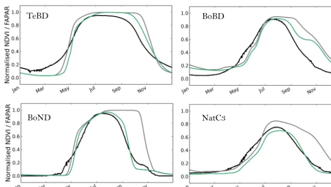
3.1.1 Step 1: assimilation of MODIS NDVI data The optimization in step 1 resulted in an improved fit to the MODIS NDVI observations for the four PFTs considered (TeBD, BoND, BoBD, NC3; see Sect. 2.4) as seen in Fig. 4,
which shows the mean seasonal cycle across the 2000–2008 period for all sites for each PFT. The most prominent change after the optimization was a substantially shorter growing season for all PFTs due to an earlier start of leaf senescence. This was caused by both a lower critical leaf age (Lagecrit)
and a higher temperature threshold for senescence (CTsenes)
(see Fig. 9). The impact on the start of leaf growth was less dramatic but important nonetheless, with a shift to a later start of leaf growth as a result of an increase in theKpheno,crit
er-TeBD BoBD
BoND NatC3
Figure 4. Mean seasonal cycle (2000–2008) of the normalized modeled FAPAR before and after optimization, compared to that of
the MODIS NDVI data, for the temperate and boreal deciduous PFTs (TeBD, BoBD, BoND and NatC3). Black=MODIS NDVI data;
gray=prior simulation (default ORCHIDEE parameters); green=posterior multi-site optimization.
ror (RMSE) of 23, 17, 58 and 19 % was achieved for TeBD, BoBD, BoND trees and NC3grasses, respectively, with the
greatest improvement for BoND trees. The mean correlation between the normalized MODIS-NDVI and modeled FAPAR time series over the 2000–2008 period increased for TeBD and BoND trees and NC3grasses (prior and posterior of 0.9
to 0.93, 0.42 to 0.91 and 0.6 to 0.66, respectively). The prior correlation of 0.55 remained similar after the assimilation for BoBD trees.
Following the improvement at the sites selected for the optimization, we evaluated the impact for each PFT at the global scale using the global median correlation between the MODIS-NDVI and the model FAPAR time series (from all pixels where the fraction of a given PFT is above 60 %; see Maignan et al., 2011). The global correlation increased for BoND trees and NC3grasses from 0.36 to 0.91 and 0.53 to
0.59 (prior to posterior), respectively. It remains stable for BoBD (0.54) or slightly increased for TeBD (0.88 to 0.89).
3.1.2 Step 2: assimilation of FLUXNET data
The optimization in step 2 brings an improvement to the simulated NEE and LE for all seven PFTs considered, with Fig. 5 showing the corresponding PFT-averaged mean NEE seasonal cycles (mean across all sites/years). NEE is overes-timated by the prior model for all PFTs on average. This is partly due to the model spin-up procedure, which brings each simulated site to a near equilibrium state with a mean NEE close to zero (i.e., no net carbon sink, see Sect. 2.1.1). This bias is significantly corrected by the optimization to match the observed carbon uptake at most sites, notably via the scal-ing of the initial soil carbon pool content at each site (param-eters KsoilC,site; Table 1), which thus significantly reduces
-4 -2 0 2
N
E
E
(g
C
m
d
)
-6 -4 -2 0 2 TropEBF TempENF TempEBF BorENFTrBE TeNE TeBE BoNE BorDBFBoBD C3grass TempDBFNC3 TeBD
(Obs PriorPosterior)
Jan Dec Jan Dec Jan Dec Jan Dec
Month
Jan Dec Jan Dec Jan Dec
-2
-1
Figure 5. Mean seasonal cycle of the net ecosystem exchange (NEE) for the different plant functional type optimized in step 2 of the assimilation. The mean across all sites for a given PFT is pro-vided for the observations (black), the posterior of step 1 (green) and the posterior of step 2 (blue).
the ecosystem respiration (Kuppel et al., 2014). Overall, the largest reductions of model–data RMSE are found in tem-perate forests (TeNE: temtem-perate needleleaf, TeBE: temtem-perate broadleaf evergreen and TeBD: temperate broadleaf decidu-ous), where the RMSE decreased by more than 25 % com-pared with the prior model. The improvements are less sig-nificant for the other PFTs, with RMSE reductions between 10 and 18 %.
In addition, the optimization increases the NEE seasonal amplitude in temperate evergreen (TeNE and TeBE) forests and temperate broadleaf deciduous (TeBD) forests, and re-duces the amplitude for boreal needleleaf evergreen (BoNE) forest and natural C3grasses (NC3), in agreement with the
nega-Time Time
Figure 6.Monthly mean atmospheric CO2concentrations after step 3 of the optimization, for several stations over the period 2002–2004 of the optimization. The observations (black), the prior model (gray) and the posterior model after step 2 (blue) and step 3 (red) are displayed. Numbers in parenthesis correspond to RMSEs.
tive NEE) in the dry season for the tropical regions (TrBE) and nearly null carbon exchange in the first months of the year for temperate regions (TeBE). These results are dis-cussed further in Kuppel et al. (2014), who used a similar optimization setup with a slightly different parameter set – see Sect. 2.3.3. Similar improvements, although of smaller amplitude, occur for the latent heat fluxes (not shown).
3.1.3 Step 3: assimilation of atmospheric CO2data The final optimization step with the atmospheric CO2
con-centrations provides a large improvement of the fit to the observed concentrations at most stations. The cost function
J was reduced through the minimization by a factor of 5.7 within 37 iterations.
Figure 6 illustrates the simulated concentrations for four stations (representative of different conditions), over the as-similation period, with the standard prior parameter vector (used in step 1), the posterior vector from step 2 (used as prior in step 3) and the posterior vector from this last step. The improvement in the fit to the observations can be quantified with the reduction in RMSE (from the prior to the posterior of step 3) – the largest reduction is at the South Pole station (73 %) and is on average around 25 % across all sites. Note that for a few stations the fit is slightly degraded (up to 10 %)
except for one Pacific site (regular ship measurements around the Equator, POCN00) for which there is a 40 % degradation, possibly due to small biases in the simulation of the ITCZ (Intertropical Convergence Zone) position in LMDz. When calculated with respect to the standard prior (used in step 1) the RMSE decrease is slightly larger on average, especially for the northern mid-to-high latitude stations. For these sta-tions the optimization performed in step 2 with FLUXNET data led to a significant improvement of the mean seasonal cycle amplitude of the atmospheric CO2data, as discussed
in Kuppel et al. (2014).
We then investigated the fit to the observed CO2
concen-trations in terms of the mean seasonal cycle and trend (see Sect. 2.4.4). With only 3 years of data the mean trend is more difficult to define as it varies between stations; however, the optimization in step 3 increases the net land carbon sink in order to match the observed trend at most stations (as ex-pected). If we take the Mauna Loa and South Pole stations that are representative of an integration of the fluxes at hemi-spheric scales, the prior CO2trend of 2.8 and 2.9 ppm yr−1,
(b) Length of CUP: relative changes (a) Seasonal amplitude: relative changes
Figure 7.Changes in the mean seasonal cycle of the atmospheric CO2concentrations after step 3 of the optimization at all atmospheric stations. Left: relative changes (in percentage) between the prior of step 3 and posterior absolute model–data differences for the amplitude of the seasonal cycle. Right: same metric but for the length of the carbon uptake period (CUP), measured as the sum of the days when the de-trended concentrations are negative (see text).
and posterior of the absolute difference between observed and modeled amplitude (1Apost−
1Aprior
/1Aprior).
They reveal an improvement in the seasonal cycle amplitude at nearly all stations of the Southern Hemisphere (≈40 % im-provement) and at the majority of the Northern Hemisphere stations (≈15 %). A few stations in northern East Asia (3) and northwestern America (4) show a small degradation of the amplitude (≈15 %). The right panel of Fig. 7 displays the changes of the CUP (see Sect. 2.4.4) expressed in terms of relative changes between prior and posterior of the absolute values of model–data differences, as it is for the amplitude. Most stations reveal an improvement of the CUP of around 20 %, which is slightly lower than the improvement for the seasonal cycle amplitude.
Finally, we verified that the improvement is valid not only at the optimization sites but also at independent atmospheric CO2stations (see Sect. 2.2.3). On average the mean RMSE
for the 24 additional sites is 10.5 ppm for the prior of step 1 (prior of ORCHIDEE), 2.8 ppm for the prior or step 3 (i.e., posterior of step 2) and 2.1 ppm for the posterior of step 3. The corresponding values for the 53 sites used for the opti-mization are 10.5, 2.45 and 1.8 ppm, respectively. The error reduction during step 3 is thus similar for both the assimi-lated and the validation data sets, further confirming that the optimization provides a global improvement of the simulated carbon fluxes.
3.2 Consistency of the stepwise optimization
The main issue with a stepwise data assimilation system (vs. a simultaneous approach) concerns the potential degradation of the model–data fit for the different data streams that are assimilated in previous steps. We noted that CO2
concen-trations were already improved when NDVI and FLUXNET data are assimilated (see Sect. 3.1.3), but we need to check if the final parameter set from step 3 leads to a degradation of
the fit to MODIS-NDVI (step 1) and to FLUXNET (step 2) data compared to the fit achieved during the respective steps and, in the case of a significant degradation, if we still have an improvement for these data streams compared to the ini-tial a priori fit.
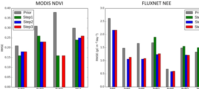
Figure 8 summarizes the performance of the model data fit for MODIS-NDVI and FLUXNET-NEE data streams for the prior and posterior of each step by evaluating the me-dian RMSE between the model and the observations across all sites. The values are calculated for each PFT separately. In this section, we keep in mind the fact that we do not opti-mize the same PFTs with FLUXNET data and with MODIS-NDVI.
3.2.1 Consistency for MODIS-NDVI
First, we notice again the significant RMSE reduction be-tween the prior and step 1, as discussed in Sect. 3.1. The fit to MODIS-NDVI (normalized data) for steps 2 and 3 shows only a significant degradation (increased RMSE) for tem-perate broadleaf deciduous (TeBD) forest, which decreases the improvement achieved in step 1 (compared to the prior) by a factor of 2. A marginal degradation for natural C3
(NC3) grassland is obtained after step 3: the RMSE increases
MODIS&NDVI& FLUXNET&NEE&
Prior Step1 Step2 Step3 Prior
Step1 Step2 Step3
RMSE (gC m day )
-1
-2
Figure 8.RMSE between model outputs and observations for two types of observations: MODIS-NDVI on the left and FluxNet-NEE on the right, for different plant functional types (PFT: TrBE, TeNE, TeBE, TeBD, BoBD, BoND, NC3) and for the prior model simulation and the posterior of each step of the assimilation framework. Missing bars correspond to the fact that no data were available to constrain a given PFT.
3.2.2 Consistency for FLUXNET data
Figure 8 again reveals the significant reduction of the RMSEs for NEE in step 2 compared to the standard prior or to the posterior of step 1 for most PFTs, except BoNE. We see only small degradations (increases) in RMSE between steps 2 and 3 for TeNE forests (from 1.06 to 1.13 g C m2d−1), TeBE forests (from 1.06 to 1.09 g C m2d−1), TeBD forests (from 1.06 to 1.13 g C m2d−1) and BoNE forests (from 0.59 to 0.60 g C m2d−1). An interesting feature to notice is that the NEE RMSE increases from the prior to the posterior of step 1 (i.e., before NEE has been used in the optimization in step 2). Using remote sensing products of vegetation ac-tivity or “greenness” (e.g., NDVI) to calibrate the phenology of ORCHIDEE thus does not always improve the simulated NEE, as they only provide a strong constraint on the timing of the leaf phenology (and thus indirectly the gross primary production, GPP) and a weak constraint on the maximum GPP but no constraint on the respiration fluxes. These rea-sons were discussed in Bacour et al. (2015), who used the same LSM and assimilation system. Overall, the reduction of the improvement of the model data fit to the NEE (step 3 vs. step 2) is marginal (limited to a few percent), thus further suggesting the consistency of our stepwise approach. Similar results are also obtained for the LE flux (not shown). 3.3 Estimated parameter values
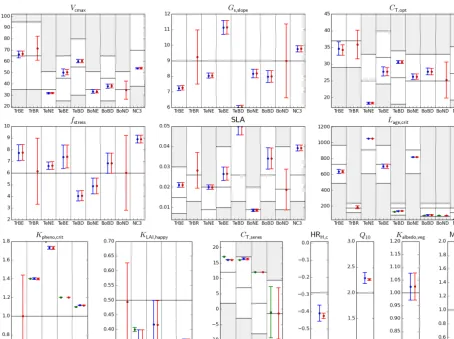
We now discuss the parameter values, focusing on the changes obtained though the successive steps. Figure 9 presents the prior and posterior values for each parameter to-gether with their associated uncertainties (estimated through Eq. 2) and the allowed range of variation. Note that nine pa-rameters are PFT dependent while four are global (non PFT dependent). For the global non-PFT-dependent parameters included in the step 2 optimization, we took the mean value and error variance (see Sect. 2.4) as the prior for step 3. Note
finally that the parameters linked to the initial soil carbon pools (KsoilC,site,KsoilC,reg) are not shown in Fig. 9 as they
are too numerous (though see Fig. A2 for the regional val-ues).
If we first consider the phenology parameters optimized in step 1 (KLAI,happy,Kpheno,crit,Lage_crit,CT ,senes; see
Ta-ble 1), we see that for most PFTs they do not change nificantly between steps 1 and 3, although they differ sig-nificantly from the prior. There are few exceptions, includ-ingKpheno,crit(the threshold for the start of the growing
sea-son) for boreal needleleaf deciduous forests andKLAI,happy
(level of carbohydrate use) for TeBD and BoBD. Note that a few phenology parameters hit one of the physical bounds, which may indicate model structural errors or model param-eter equifinality. For most phenology paramparam-eters, the uncer-tainties are strongly reduced during their first optimization (step 1), except for a few cases likeCT ,senes for C3
grass-land. Note finally that a more in depth spatiotemporal vali-dation demonstrated the generality of the optimized phenol-ogy parameters across multiple sites (for further details see MacBean et al., 2015).
For the photosynthesis parameters (Vcmax,Gs,slope,cT ,opt,
SLA,fstress; see Table 1), we find a similar result with small
changes between steps 2 and 3, but still a significant depar-ture from the prior values. Most parameters are well con-strained by the inversion, with posterior uncertainties that are greatly reduced compared to the prior, except for TrBR forest and BoND forest for which there is nearly no constraint on
Gs,slope andfstress(see Table 1).
The non-PFT-dependent respiration-related parameters (HRH,c,Q10, MRb) mostly change in step 2 and only slightly in step 3 (with an additional reduction of the error) in order to fit the large-scale constraint provided by the atmospheric ob-servations. The values of the scalar of the initial soil carbon pools size for the FLUXNET site optimizations (KsoilC,site,
Figure 9.Prior and posterior parameter values and uncertainties for a set of optimized parameters (nine PFT dependent and four non-PFT dependent). The prior value corresponds to the horizontal black line and the physical allowed range of variation to the “y” range (i.e., the white zone). For PFT-dependent parameters, there are nine sub-plots corresponding to PFTs that were optimized (except forKpheno,critwith only five PFTs). For each parameter, there are three estimated values for the three successive steps: step 1: assimilation of MODIS-NDVI data (green symbol); step 2: adding FLUXNET data (blue symbol); step 3: adding atmospheric CO2data (red symbol). The parameter values are depicted with the symbols and the estimated uncertainties with the vertical line (±σ).
average, in order to decrease the heterotrophic respiration (see Kuppel et al., 2014 for additional discussion). In step 3 the same scalars that were defined for an ensemble of large regions (KsoilC,reg) have decreased in the Southern
Hemi-sphere (less than 10 %; see Fig. A2 in Appendix A3) and slightly increased in the Northern Hemisphere (around 1 %), to achieve a better match to the atmospheric CO2 growth
rate and north–south gradient. Importantly, we notice that for step 3, the fit to the atmospheric CO2concentrations
(es-pecially to the trend) is achieved mainly by small changes in KsoilC,reg and in few other respiration-related
parame-ters. Note finally that the parameter controlling the albedo (Kalbedo,veg), modified with the FLUXNET observations only
(see Sect. 2.4), is not well constrained by the optimization (only a small reduction in uncertainty). Overall, most param-eters appear to be well constrained when first optimized, with only small changes in the following steps. This suggests that
the targeting of different parameter subspaces in the various optimization steps was well chosen.
3.4 Estimated carbon fluxes and uncertainties
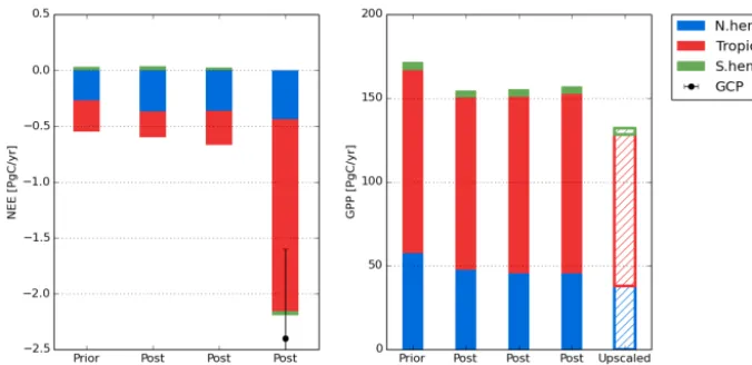
Figure 10.Left: net ecosystem exchange (NEE) for three regions (north of 35◦N, tropics, south of 35◦S) for the prior model, and after each step of the optimizations (mean over 2002–2004). The NEE estimate from the Global Carbon Project (GCP) for the same period (Le Quéré et al., 2015) is provided for step 3 with its error bar. Right: same but for gross primary production (GPP) where the data-driven estimate (MTE product using FluxNet data; Jung et al., 2011) is provided for comparison.
3.4.1 Large-scale annual mean net fluxes
The mean annual carbon fluxes (NEE) for the globe, northern extra tropics, tropics and southern extra tropics are reported in Fig. 10 for the 2000–2009 decade for the prior and pos-terior model simulations for all steps. We ran the optimized model over the full decade in the 2000s in order to compare with one other estimate of the land surface residual from the GCP (Le Quéré et al., 2015) over the same decade. The prior NEE indicates a total sink of 0.5 PgC yr−1over this period, from both the northern and tropical regions. Such a prior sink is due to the increase of atmospheric CO2 during the
transient simulation following the spin-up (1990–2009, see Sect. 2.3.1) and climate variability. Changes from the prior are rather small in step 1 (assimilation of MODIS NDVI) with an increase of the northern sink by 0.12 PgC yr−1and a decrease of the tropical sink by 0.05 PgC yr−1 (Fig. 10). Step 2 (assimilation of FLUXNET data) does not signifi-cantly change the net C sink from step 1, with only a small in-crease in the tropical sink by 0.1 PgC yr−1. The assimilation of atmospheric CO2data in step 3 provides a large-scale
con-straint, as already discussed, and increases the total land sink to 2.2 PgC yr−1, a value in much closer agreement with the estimate by the GCP. A larger tropical NEE uptake is respon-sible for the large increase of the terrestrial biosphere C sink (from 0.3 PgC yr−1in step 2 to 1.7 PgC yr−1) while the sink
in the north increases by less than 0.1 PgC yr−1. The
compar-ison with the GCP number should be taken with caution. The ORCHIDAS estimated sink includes all effects (natural and anthropogenic), since we used atmospheric CO2as a global
constraint. Thus, the optimized parameters must account for any missing processes like nitrogen limitation or a proper de-scription of agricultural processes and management. How-ever, the GCP number is only for the anthropogenic uptake,
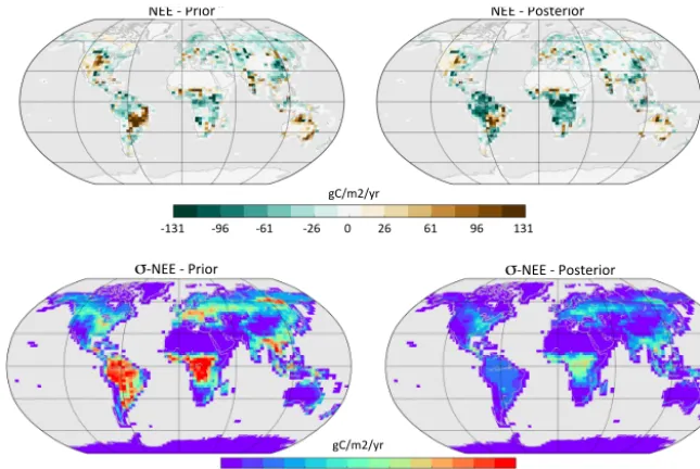
excluding the pre-industrial sink due for instance to river ex-port of carbon (around 0.45 PgC yr−1; Regnier et al., 2013). 3.4.2 Spatial distribution of the annual mean net flux Figure 11 shows the spatial distribution of NEE averaged over 2002–2004 for the standard prior and posterior after step 3. The large tropical net land carbon sink that is inferred in step 3 is mainly explained by an increase of the carbon uptake for the tropical forests of the Amazon basin and equa-torial Africa, as well as a decrease of the carbon release on the southern edge of the Amazon basin (tropical rain-green forests and grasses). In the northern mid-to-high latitudes only smaller regional changes from the prior occur. For Eu-rope, most of north Asia and Canada, the strength of the C sink slightly decreased from the prior (up to 30 g C m2yr−1), while for central USA the strength of C source slightly de-creased. If we now consider the uncertainties on the net an-nual carbon flux that arise from the parameter uncertainty (second row of Fig. 11; Eq. 2), we observe a very large reduction (compared to the prior) in the monthly flux un-certainty (averaged over the 3 years used in step 3) over tropical forests. It is reduced by a factor 4 with initial val-ues around 150 g C m2yr−1and posterior values between 22 and 66 g C m2yr−1. For mid-to-high latitude boreal ecosys-tems, the uncertainty reduction is smaller, but the posterior errors are slightly lower than over the tropics, between 18 and 55 g C m2yr−1.
3.4.3 Large-scale annual mean gross primary production
poste-NEE - Prior NEE - Posterior
σ-NEE - Prior σ-NEE - Posterior
-131 -96 -61 -26 0 26 61 96 131 gC/m2/yr
22 44 66 88 110 132 154 176 gC/m2/yr
NEE - Prior NEE - Posterior
σ-NEE - Prior σ-NEE - Posterior
Figure 11.Simulated annual net carbon exchange (NEE) for the land ecosystems prior to any optimization (left column) and after step 3 of the optimization process (right column). Upper figures correspond to the mean NEE (in g C m−2yr−1) over the assimilation period (2001– 2003) and lower figures to the associated monthly flux uncertainties (averaged over the whole period and expressed in g C m−2yr−1) due to the parameter uncertainties (see text).
rior of step 1, 2 and 3, respectively. The small overall de-crease (9 %) brings the GPP slightly closer to the estimate by Jung et al. (2011), around 120 PgC yr−1, based on a statisti-cal model tree ensemble (MTE) that upsstatisti-caled the in situ flux measurements (resulting from the partition of measured NEE into GPP and total ecosystem respiration). The decrease in GPP occurs mainly in the Northern Hemisphere after step 1 (−10 PgC yr−1) following the decrease in Vcmax (Fig. 9)
while it remains relatively stable over the tropics across all steps. Note that (i) the study of Welp et al. (2011) suggests a GPP around 150 PgC yr−1, similar to our estimate, based on measurements of18O/16O ratio in atmospheric CO2and
(ii) Koffi et al. (2012) found optimized GPP of 146 PgC yr−1 from a CCDAS using the BETHY model.
3.4.4 Aboveground forest biomass
We analyze the impact of the optimization on the forest aboveground biomass at equilibrium (i.e., after spin-up; see Fig. 12) as an example of the impact on model C stocks, and compare the simulated values, for the same three lati-tude bands than above, to the estimate based on field obser-vations and remote sensing data. This product, which was produced in the GEOCARBON project (and thus is referred to by the same name), integrates a pan-tropical biomass map (Avitabile et al., 2016) with a boreal forest biomass product (Santoro et al., 2015).
For the northern extra tropics, the prior aboveground C stock (∼180 PgC) is reduced by the optimization to 140 PgC, mainly through the decrease of the growing season length
Figure 12. Aboveground forest biomass data for the prior OR-CHIDEE model and after step 1, step 2 and step 3 of the opti-mization process. Estimates from satellite observations (Santoro et al., 2015) and referred as “GEOCARBON” (following the EU-GEOCARBON project) are provided for comparison.
in step 1 with the assimilation of MODIS-NDVI. The sig-nificant decrease in GPP during step 1 (18 %) led indeed to a similar decrease of the forest biomass (16 %). Parame-ter changes through the assimilation of FLUXNET and CO2