Volume 14 - Article 1 | Pages 1–26

in the population sciences published by the Max Planck Institute for Demographic Research Konrad-Zuse Str. 1, D-18057 Rostock·GERMANY www.demographic-research.org

DEMOGRAPHIC RESEARCH

VOLUME 14, ARTICLE 1, PAGES 1-26

PUBLISHED 24 JANUARY 2006

http://www.demographic-research.org/Volumes/Vol14/1/ DOI: 10.4054/DemRes.2006.14.1

Research Article

Tempo effects in mortality:

An appraisal

Michel Guillot

c

1 Introduction 2 2 The existence of tempo effects in mortality 4 3 Bongaarts and Feeney’s tempo-adjusted life expectancy 7 4 Evaluating Bongaarts and Feeney’s “proportionality” assumption 8 5 Bongaarts and Feeney’s definition of changes in period mortality

conditions

12

6 Assessing indicators of period mortality conditions: eo vs. CAL 17

7 Conclusion 22

8 Acknowledgements 23

Tempo effects in mortality:

An appraisal

Michel Guillot1

Abstract

This study examines the existence of tempo effects in mortality and evaluates the proce-dure developed by Bongaarts and Feeney for calculating a tempo-adjusted life expectancy. It is shown that the performance of Bongaarts and Feeney’s index as an indicator reflect-ing current mortality conditions depends primarily on specific assumptions regardreflect-ing the effects of changing period mortality conditions on the timing of future cohort deaths. It is argued that, currently, there is no clear evidence about the existence of such effects in actual populations. This paper concludes that until the existence of these effects can be demonstrated, it is preferable to continue using the conventional life expectancy as an indicator of current mortality conditions

1_{Center for Demography and Ecology, University of Wisconsin-Madison, 1180 Observatory Drive, Madison,}

1. Introduction

There are three main uses of period indicators – such as the total fertility rate (TFR) or the life expectancy at birth (_e0) – in demography. First, period indicators are used as sum-maries of period age-specific rates, in order to allow easy comparisons of arrays of rates across populations and time periods. For example, aTFRthat is lower in Population A than in Population B implies that at least one age-specific fertility rate is lower in Popu-lation A. In order to give a metric to these summary measures that is easy to interpret in terms of the underlying demographic processes, demographers use the classic synthetic-cohort scenario, which simulates a synthetic-cohort of individuals exposed throughout their entire life to the specific rates of one particular period. This transforms a set of period age-specific mortality rates, for example, into years of life, interpreted as the life expectancy at birth “under current rates”.

Second, period summary measures are used as indicators of current “conditions”, which can be defined as all underlying factors affecting demographic behavior. For ex-ample, an increase in life expectancy is often interpreted as a sign that progress is being made with respect to public health, medical technology, personal health behaviors, living standards, or other factors affecting survival. One way to conceptualize how current con-ditions may produce a certain level of a demographic indicator is to hypothesize about a scenario in which current conditions stay constant in the future. Under this scenario, one would expect period demographic indicators to eventually stabilize at a level that would be the product of these constant conditions. In the remainder of this paper, I will refer to levels of demographic indicators that would eventually be observed in the population if current conditions remained constant in the future as the “stationary-equivalent” levels, or levels “under current conditions”.

Third, period summary measures are used as proxies for tracking the changing be-havior of real cohorts in the absence of complete cohort information. For example, an increase in the period life expectancy at birth is often interpreted as an indication that “we are living longer”, i.e., that life expectancy is also increasing for real cohorts of individu-als.

that year experienced such high fertility levels (the highest cohortTFRamong cohorts active in 1955 is3_.2, for the cohort born in 1930). Also, the below-replacement period TFRs currently observed in a number of countries may poorly reflect current fertility conditions, because cohorts may be currently delaying their births while retaining fertility goals at or above replacement. If the conditions affecting individuals’ completed fertility remain constant in these countries, the cohort TFR may eventually stabilize at a level that is higher than the one indicated by current periodTFRs. Tempo effects thus pose a challenge for the interpretation of levels and trends in periodTFRs.

Tempo effects have been extensively studied for fertility and marriage (Ryder, 1956, 1964, 1980; Keilman, 1994; Bongaarts, 1998, 1999; Kohler, 2002; Goldstein, 2003; Winkler-Dworak and Engelhardt, 2004). Various approaches have been proposed to ad-just period measures for tempo effects. It is important to state that the solution for the adjustment may vary depending on the purpose of the correction, i.e., measuring period conditions or tracking real cohort behavior. In fertility, the first purpose involves estimat-ing the level at which theTFRwould eventually stabilize if factors affecting individuals’ completed fertility remained constant at the levels of a particular period. The second purpose involves estimating theTFRthat would have been observed during that partic-ular period if cohorts had not modified the timing of their births, while retaining their potentially changing completed fertility. These two scenarios differ and may thus yield different solutions. Differences in objectives explain in part why different procedures for tempo adjustments in fertility have yielded different results.

More recently, the concept of tempo effects has been applied to mortality (Bongaarts and Feeney, 2002, 2003, 2005). The authors argue that the conventionally-calculated period life expectancy at birth is affected by tempo effects whenever mortality is changing. They propose an alternative period measure of longevity, which they claim adjusts for tempo effects. Although not explicitly stated, the purpose of the adjustment is to obtain a measure that better reflects current conditions, i.e., the level at which the life expectancy at birth would eventually stabilize if mortality conditions, defined as all factors affecting survival, remained constant at current levels.

2. The existence of tempo effects in mortality

There are interesting parallels between mortality and fertility with regards the study of tempo effects. The mortality index for which the parallel best applies is the total mortality rate (TMR) (Bongaarts and Feeney, 2003). In a cohort (real or synthetic), theTMRis the number of lifetime deaths divided by the initial size of the cohort. In a life table with a radix of one, theTMR can be calculated by adding all age-specific life table deaths. Obviously, theTMR in a cohort, real or synthetic, is invariably one. The following equation pertains to a real cohort born at timet:

T M Rc(t) =

_∞

0 dc(x, t)dx

(1)

where_dc(_{x, t})is the number (or proportion) of deaths at age_xfor a cohort born at time_t (radix= 1).

TheTMRcan also be calculated in a cross-sectional fashion by calculating for each cohort the proportion of deaths occurring during a particular period, and by summing these proportions across all cohorts:

T M R(t) =

_∞

0 dc(x, t−x)dx

(2)

The periodTMRcan be interpreted as the proportion of cohort deaths that are occurring during periodt. If all cohorts have the same age distribution of deaths, the periodTMRis constant at1.00. If the age distribution of deaths changes from cohort to cohort, however, the periodTMRdeviates from one. For example, if cohort deaths are being progressively spread out over a longer period of time, with smaller proportions occurring during a given period, the periodTMR is less than one. This means that less than 100% of cohort deaths are occurring during period_t, which is a sign that cohort deaths are being delayed, i.e., that mortality is declining. Conversely, the periodTMRis greater than1_.00during periods of increased mortality, when increased proportions of cohort deaths are occurring at the same time.

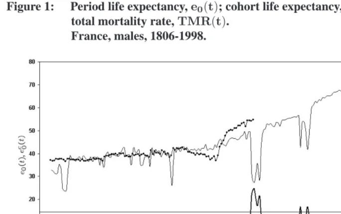
Figure 1: Period life expectancy,e₀(t); cohort life expectancy,ec₀(t); and period total mortality rate,TMR(t).

France, males, 1806-1998.

Note: Data source: Vallin-Mesl´e database. http://www.ined.fr/publications/cdrom vallin mesle/contenu.htm Note:ec₀(t)is plotted at time when the cohort was born.

eventually be observed if current mortality conditions remained constant in the future. Indeed, under this constant-conditions scenario, one would expect the age distribution of deaths to be eventually identical for all cohorts, and the periodTMRto reach a value of

1.00eventually. The periodTMRis also a poor indicator of the trend in the cohortTMR, which is constant at1_.00for all cohorts. Making a parallel with fertility, it can be stated that the periodTMRis affected by tempo changes, defined as changes in the timing of deaths within cohorts. Unlike the cohortTFR, however, there are no quantum variations in the cohortTMR, since it is constant at1_.00. This implies that deviations from1_.00in the periodTMRcan be entirely attributed to tempo effects, and that a “tempo-adjusted” periodTMRnecessarily equals1_.00.

Figure 2: Period life expectancy,e₀(t); cohort life expectancy,ec₀(t); and period total mortality rate,TMR(t).

Sweden, females, 1752-1998.

Data source: Human Mortality Database. www.mortality.org. Note:ec₀(t)is plotted at the time(t)when the cohort was born.

there are a few years – the WWI years – during which period_e0levels have no relevance for any particular cohort. During these years, many cohorts had elevated mortality risks at the same time, resulting in period life expectancies as low as27_.2years in 1915. But these elevated risks were relatively short-term, and no actual cohort contributing deaths during these years have experienced such low life expectancy levels (the lowest cohort life expectancy among contributing cohorts is37_.0years for the cohort born in 1895). In a sense, the sudden decline in life expectancy in 1915 gives an exaggerated indication of mortality change occurring within cohorts. Changes in cohort mortality levels would have been poorly predicted on the basis of these large drops ine0. This discussion of trends in period life expectancy has parallels with discussions of trends in the periodTFRand the difficulty to use this measure as an indicator of real changes in cohort completed fertility.

expectancy are of little use for answering that question, because cohorts are exposed to constantly-changing period conditions.

3. Bongaarts and Feeney’s tempo-adjusted life expectancy

The goal of Bongaarts and Feeney’s alternative measure of survival is precisely to resolve potential discrepancies between period levels and stationary-equivalent levels of life ex-pectancy. As said earlier, the goal of their tempo-adjusted measures is not to better track real changes in cohort life expectancy, so I will not discuss here how their approach per-forms this task. There are a number of papers in this volume and elsewhere which deal with this somewhat different issue (Guillot, 2003; Schoen and Canudas-Romo, 2005; Goldstein, 2006).

Bongaarts and Feeney (referred to as BF in the remainder of the paper) compare three mortality indexes:

CAL(t) =

_∞

0 pc(x, t−x)dx

(3)

where_pc(_{x, t}−_x)is the proportion of cohort survivors aged_xat time_t.

MAD(t) =

_∞

0 x·dc(x, t−x)dx

∞

0 dc(x, t−x)dx

(4)

M4(t) =

_∞ 0 exp − _x 0

µ(a, t) T M R(t)da

dx (5)

where_µ(_{a, t})is the force of mortality at age_aat time_t.

The first index,CAL(_t)(= cross-sectional average length of life), sums actual pro-portions of cohort survivors at time_t, rather than proportions of survivors in the synthetic cohort at time_tas in the case of_e0(_t). ThusCALtakes into account all mortality rates previously experienced by cohorts whose survivors are present in the population at time

t. This index, which is described in detail elsewhere (Brouard, 1986; Guillot, 1999, 2003, 2005), has been used primarily for examining the impact of mortality change on popula-tion growth.

The second index,MAD(_t), is the mean age at death that would be observed at time

The third index,_M4(_t), is a period life expectancy at birth where all age-specific death rates are adjusted by a factor1_/TMR(_t). If theTMRis equal to_.8, each death rate will be adjusted upwards by a factor1_.25, and_M4(_t)will be lower than the actual_e0(_t).

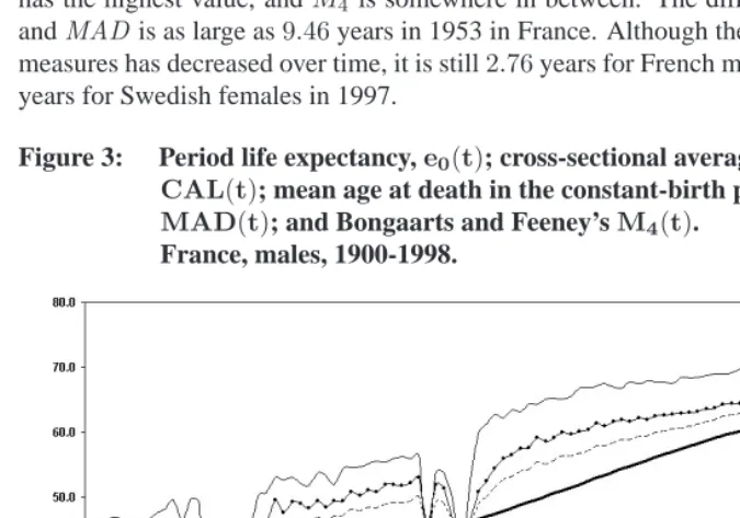
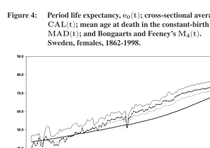
An important feature of these summary indexes of mortality is that when mortality is constant over time, thenCAL(_t) = MAD(_t) = _M4(_t) = _e0(_t). If mortality varies, however, these indexes diverge. In particular, if age-specific mortality rates have been steadily declining,_e0will be systematically higher thanCAL,MADor_M4.

Bongaarts and Feeney calculate these three indexes in populations where mortality has changed overtime. They demonstrate thatCAL =MAD =_M4under a specific pattern of mortality change, which they claim is a good approximation of the current situation in low-mortality populations. This quantity is then interpreted as a tempo-adjusted life expectancy at birth. These two propositions are examined successively in the following sections.

4. Evaluating Bongaarts and Feeney’s “proportionality” assumption

The first assumption proposed by Bongaarts and Feeney involves a quantity described by Preston and Coale (1982) and Arthur and Vaupel (1984). This quantity may be called an age intensity,_ν∗:

ν∗(x, t) =−∂pc(x, t−x)/∂x

pc(x, t−x) . (6)

In Equation (6),_ν∗is the rate at which the proportion of cohort survivors in a population at time_tvaries from one age to the next. It also corresponds to the age intensity of the constant-birth population. It is in fact a special case of Arthur and Vaupel’s age intensity,

ν, which applies to the more general case of populations with varying births and open to migration.

In their paper, Bongaarts and Feeney (2003) demonstrate thatCAL(_t) =MAD(_t) =

M4(t)if at time_tthe age intensity_ν∗(_{x, t})is proportional to_µ(_{x, t}), i.e., if the following equation holds:

the amount of the shift, in years, between_t1and_t2(Bongaarts and Feeney, 2002). For ex-ample, the proportionality assumption would be met if the proportion of cohort survivors at age80in 2000 was equal to the proportion of cohort survivors at age78in 1995 (i.e., a 2-year shift in5years), and if this correspondence could be established for all cohorts.

While it is true that if Equation (7) holds at time_t, thenMAD(_t) =CAL(_t) =_M4(_t), there are deviations from the proportionality assumptions in real populations which pro-duce important discrepancies between the three indicators. This can be shown by calcu-lating the three indicators in real populations, without making any assumption about the pattern of mortality change.

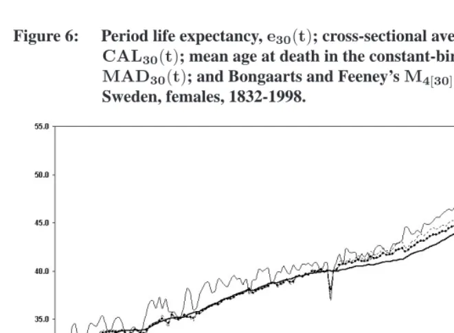
Figures 3 and 4 show that among French males and Swedish females, there are impor-tant differences between the three indicators. Typically,CALhas the lowest value,MAD has the highest value, andM4 is somewhere in between. The difference betweenCAL andMADis as large as9_.46years in 1953 in France. Although the gap between the two measures has decreased over time, it is still2_.76years for French males in 1998, and2_.08 years for Swedish females in 1997.

Figure 3: Period life expectancy,e₀(t); cross-sectional average length of life, CAL(t); mean age at death in the constant-birth population, MAD(t); and Bongaarts and Feeney’sM₄(t).

France, males, 1900-1998.

Figure 4: Period life expectancy,e₀(t); cross-sectional average length of life, CAL(t); mean age at death in the constant-birth population, MAD(t); and Bongaarts and Feeney’sM₄(t).

Sweden, females, 1862-1998.

sensitive to variations in period mortality, with a trajectory somewhat parallel to that of the period life expectancy at birth, although at a lower level. In contrast,CALis much less reactive to period variations in mortality. Since in real populationsCAL,MADand

M4offer a different picture of changes in mortality over time, these three indexes should not be interpreted interchangeably. In particular, CAL should not be interpreted as a population mean age at death purged of changes in cohort size (MAD). Even if today, the difference between the two indexes is not as large as earlier (though still significant), they remain distinct conceptually.

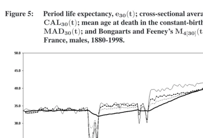
Figure 5: Period life expectancy,e₃₀(t); cross-sectional average length of life, CAL30(t); mean age at death in the constant-birth population, MAD30(t); and Bongaarts and Feeney’sM_4[30](t).

France, males, 1880-1998.

Note: Likee30(t),CAL30(t),MAD30(t), andM_4[30](t)represent a number of additional years expected to be lived above age30, given survival to age30.

In reality, mortality below age30is not negligible, especially when considering earlier decades of the twentieth century. Even in 1998 among French males, mortality below age

Figure 6: Period life expectancy,e₃₀(t); cross-sectional average length of life, CAL30(t); mean age at death in the constant-birth population, MAD30(t); and Bongaarts and Feeney’sM_4[30](t).

Sweden, females, 1832-1998.

Data source: Human Mortality Database. www.mortality.org. Note:ec₀(t)is plotted at the time(t)when the cohort was born.

5. Bongaarts and Feeney’s definition of changes in period mortality

conditions

While departures from the proportionality assumption raises practical issues with the es-timation of BF’s adjusted life expectancy, there are more fundamental considerations to examine in order to evaluate the interpretation ofCAL,MADor_M4as tempo-adjusted indicators. These considerations apply even if the proportionality assumption is met. SinceCAL = MAD = _M4 under the proportionality assumption, this section focuses on the behavior ofCAL only. I chooseCAL, because unlikeMAD or_M4, it has rel-evant properties (for example, Equation (8) later in this paper) that do not require any assumption about the pattern of mortality change.

respect to the risk of death. Therefore, it is assumed that changes in period age-specific mortality rates completely reflect changes in period mortality conditions. Similarly, it is assumed that when period mortality conditions stop changing, period age-specific mortal-ity rates – or_e0– become constant. Under this assumption, the period life expectancy at birth, as traditionally calculated, is an unbiased indicator of period mortality conditions, and no adjustment is needed.

As in the classic approach, BF assume that populations are homogeneous with respect to the risk of death, but they address mortality change differently. They define period mortality changes in terms of changes overtime in the_pc(_{x, t}−_x)curve. According to them, a change in mortality conditions during a certain period is indicated by a change in_pc(_{x, t}−_x), producing a change in the value ofCAL. Conversely, they assume that mortality conditions stop changing whenever the curve_pc(_{x, t}−_x)– or whenCAL(_t)– becomes constant (Bongaarts and Feeney, 2002, p.17).

BF’s definition of mortality change implies that, as a result of new mortality conditions appearing during a given period, all future cohort deaths are delayed by a certain amount of time. These delays in future cohort deaths accumulate over time as mortality conditions keep improving. When mortality conditions stop improving, no additional delay occurs, which implies that the delays in future cohort deaths, already accumulated by previous mortality change, remain unchanged.

gen-erating delays in future cohort deaths. It does not refer to the time when these delays are actually experienced, because these delays can indeed be experienced many years later.

Figure 7: Lexis diagram illustrating Bongaarts and Fenney’s scenario of mortality change.

Diagram A: New conditions appear at timeT:

Note: The quantities in the Lexis areas refer to deaths in cohort life tables with a constant radix at age zero. The arrows indicate the proportions of cohort deathsλ(T)that “migrate” to the following year as a results of the new conditions appearing in yearT. These proportions apply to the stationary deathsDxof yearT−1.

D

x = Dx · [1−λ(T)] + Dx−1 ·λ(T)

According to this scenario of mortality change, theTMRduring yearT is equal to

(1−λ(T)). However, if cohorts experience no additional delays in the timing of their future deaths, i.e., if mortality conditions stop changing according to BF’s definition of mortality change, constant numbers of cohort deaths,_Dx, reemerge as early as the year

T+ 1. This implies that, starting in year_T + 1, aTMRof1_.00is reestablished,CAL becomes constant, and_e0(_t) = _ec₀(_t) = CAL(_t). The life expectancy at birth during year_T will be higher than the new constant level starting at_T+ 1, because unlike year

Figure 7 (continued): Diagram B: New conditions appear at timeT+1

Note: The quantities in the Lexis areas refer to deaths in cohort life tables with a constant radix at age zero. The arrows indicate the proportions of cohort deathsλ(T+ 1)that “migrate” to the following year as a results of the new conditions appearing in yearT+ 1. These proportions apply to the stationary deathsD_x that would have been observed during the yearT+ 1and subsequently if no further mortality change had occurred after timeT(as shown in Diagram A).D_x = D_x · [1−λ(T+ 1)] + D_x−1 ·λ(T+ 1)

Mortality conditions, however, may not remain constant but be replaced by new mor-tality conditions appearing during year_T + 1 (Diagram B). These new conditions, ac-cording to BF, generate additional delays in cohort deaths, illustrated by a second set of arrows indicating the proportions of cohort deaths_λ(_T+ 1)that are postponed to the fol-lowing year as a result of the new mortality conditions of year_T + 1. These proportions apply to the deaths_Dxthat would have been observed during year_T+1and subsequently if no further mortality change had occurred after time_T (a counter-factual scenario that corresponds to the situation described in Diagram A).

appearing every year and creating delays in cohort deaths which would come in addition to the delays already accumulated as a result of previous mortality change.

This example illustrates the implications of BF’s conception of mortality change. The first implication is that changes in mortality conditions are entirely indicated by deviations from1_.00in theTMR. When new period mortality conditions appear, theTMRdeviates from1_.00, and the quantity(1−TMR)indicates the proportion of cohort deaths that are postponed to the following year as a result of these new conditions, or equivalently, the amount of the delay. As period mortality conditions stop changing, aTMRof1_.00is im-mediately reestablished. Similarly, changes in mortality conditions are entirely indicated by changes inCAL, because there is a direct connection between changes inCALand levels of the periodTMR(Guillot, 2003, p.53):

T M R(t) = 1−dCAL(t)

dt (8)

(Note that unlike BF’s similar equation (Bongaarts and Feeney, 2003, p.13129, Equation [8a]), Equation (8) does not require any assumption.)

The second implication of BF’s conception of mortality change pertains to the inter-pretation ofCALas a stationary-equivalent life expectancy. BF’s assumption about the effect of new mortality conditions on the timing of future cohort deaths produces a situa-tion in whichCALbetter reflects current mortality conditions, becauseCALcorresponds to the life expectancy at birth that would eventually be observed in the population if mor-tality conditions stopped changing (i.e., if cohorts experienced no additional delays in the timing of their future deaths). In Diagram B of Figure 7, the period life expectancy at birth observed during year_T+ 1does not reflect well the new mortality conditions emerging during that year, because it is different from the constant level of life expectancy at birth that would be observed starting in yearT + 2if mortality conditions remained constant. In reality, new mortality conditions may appear in yearT+ 2and subsequently. Nonethe-less, no matter what happens during yearT+ 2, the level ofCALobserved on January 1 of year_T + 2indicates this stationary-equivalent level of mortality.

BF’s tempo-adjusted life expectancy is thus a stationary-equivalent period life ex-pectancy that is consistent with their definition of mortality change, based on the behav-ior of_pc(_{x, t}−_x). In general terms, if _pc(_{x, t}−_x)becomes constant at time_t, then

p(x, t) = pc(x, t−x). Therefore, if_pc(_{x, t}−_x) becomes constant, _e0 immediately adjusts to the correspondingCALlevel and remains constant thereafter.

One can note here that this scenario of constant mortality conditions is possible only if the function_pc(_{x, t}−_x)is monotonically decreasing. This assumption is less restrictive than BF’s proportionality assumption, and allows for the proportion of postponed deaths,

a stationary-equivalent life expectancy, is that these age-specific delays in future cohort deaths generated by the new conditions of year_T– which we can denote_λ(_{x, T})– must be identical for all cohorts. For example, new mortality conditions of year_Tmust gener-ate delays in deaths of age80for the cohort age40at time_T that are equal to the delays in deaths of age80for the cohort aged70at time_T. In other words, age-specific delays need to remain constant with time in the constant-condition scenario. In Figure 7A, the proportions of deaths transferred to the following year as a result of new mortality con-ditions of year_T, illustrated with the arrows, may vary vertically, but must be constant horizontally. This insures that_e0adjusts toCALin BF’s scenario of constant mortality conditions.

6. Assessing indicators of period mortality conditions:

e

vs.

CAL

The assessment of BF’s tempo-adjusted life expectancy (apart from discussing the ade-quacy of the proportionality assumption) comes down to determining whether new mor-tality conditions generate a new set of period age-specific death rates, as traditionally believed, or whether these new conditions generate delays in the timing of future cohort deaths, as illustrated in Figure 7. In particular, it comes down to determining whether cohorts would stop experiencing additional delays in the timing of their future deaths if mortality conditions stopped changing. In general terms, it comes down to determining whether levels and trends in period mortality conditions are better reflected by changes in life expectancy or changes inCAL.

In order to contrast these two views, one first needs to recognize that life expectancy andCALare not independent of one another. In particular, it can be shown that variations inCALdepend in part on differences between proportions of survivors in the synthetic cohort at time_tand proportions of survivors in real cohorts at time_t(Guillot, 2003, p.53):

dCAL(t)

dt =

_ω

0 µ(x, t)[p(x, t)−pc(x, t−x)]dx

(9)

where_ωis the age at which_p(_{x, t}) =_pc(_{x, t}−_x) = 0.

Under steady mortality decline,_p(_{x, t})tends to be greater than_pc(_{x, t}−_x), andCAL tends to increase. In fact, if_p(_{x, t})=_pc(_{x, t}−_x)for any_xin the interval(0_{, ω})(which happens for most years in France and Sweden), the direction of the change inCALwill be determined by the sign of the difference between_e0andCAL:

dCAL(t)

dt = ¯µ(t)[e0(t)−CAL(t)] (10)

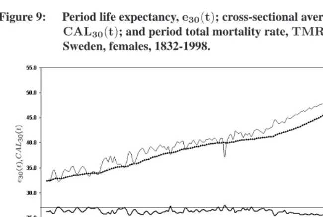
Figure 8 and 9 show trends in life expectancy and CALamong French males and Swedish females. In order to examine these trends in the context of BF’s discussion of tempo effects, these figures use mortality information above age30only, but similar correspondences betweenCALand life expectancy would be observed if all ages were taken into account. As expected, the direction of the change inCALis related to whether life expectancy is above or below the corresponding value ofCAL. These figures also illustrate the relationship betweenCALchange and theTMRlevels (Equation (8)).

Figure 8: Period life expectancy,e₃₀(t); cross-sectional average length of life, CAL30(t); and period total mortality rate,TMR₃₀(t).

France, males, 1880-1998.

Equations (9) and (10), illustrated in Figures 8 and 9, allow us to contrast two dif-ferent views of mortality change above age30. The classic view implies that changes in mortality conditions at these ages is indicated by changes in_e30, and thatCAL₃₀simply “reacts” to these variations, depending on whether_e30is above or belowCAL₃₀during a given year. According to this view, if current conditions stopped changing,_e30would remain constant whileCAL₃₀would gradually increase towards_e30, as expected from Equation (9). This view implies thatCAL₃₀is a biased indicator of stationary-equivalent life expectancy, because if mortality conditions stopped changing,_e30would remain con-stant whileCAL₃₀would continue changing.

what-Figure 9: Period life expectancy,e₃₀(t); cross-sectional average length of life, CAL30(t); and period total mortality rate,TMR₃₀(t).

Sweden, females, 1832-1998.

ever trajectory CAL₃₀ is taking. According to this view, _e30 is a biased indicator of stationary-equivalent life expectancy, becauseCAL₃₀ would remain constant while_e30 would change if mortality conditions stopped changing.

Another way to contrast these two views is to examine the equation for theTMR. Equation (11) is a modified version of Equation (2) in which cohort deaths at time t are expressed in terms of cohort survivors exposed to the force of mortality at time_tand in which only ages30and above are taken into account (i.e.,_pc(30_{, t}−30) = 1):

T M R30(t) =

_∞

30 pc(x, t−x)·µ(x, t)dx

(11)

As we saw earlier, theTMRwill deviate from1_.00whenever the timing of deaths is changing from cohort to cohort. No matter how we define mortality conditions, if period mortality conditions stopped changing, one would expectTMR₃₀to eventually reach the stationary value of1_.00. The stationary-equivalent periodTMR₃₀, orTMR₃₀(∞), can thus be expressed for a given year as TMR₃₀(_t) divided by itself. This produces the following equation:

TMR30(∞) = _TMR1 30(t)

_∞

30 pc(x, t−x)·µ(x, t)dx

The conventional approach would attribute deviations inTMR₃₀(_t)to the fact that the proportions of cohort survivors, representing individuals exposed to past mortality levels, tend to be smaller than proportions of survivors in the synthetic cohort for year

t, while_µ(_{x, t})adequately represents current mortality conditions. If current mortal-ity conditions stopped changing, the stationary-equivalentTMR₃₀(∞)of1_.00would be reached through a progressive increase in_pc(_{x, t}−_x), while_µ(_{x, t})would stay constant at current levels. In contrast, BF assume that, if mortality conditions stopped changing, the stationary-equivalentTMR₃₀(∞)of1_.00would be reached through a change in the force of mortality by a factor1_/TMR₃₀(_t), while_pc(_{x, t}−_x)would stay constant at current levels. They are able to entirely attribute the correction factor of1_/TMR(_t)in Equation (12) to_µ(_{x, t})because of their assumption of cohort-invariant delays of future cohort deaths in the constant-condition scenario. (This adjustment ofµ(x, t)appears in Equation (5) forM4.) In sum, both views agree thatTMR₃₀(t)is biased an indicator of the stationary-equivalentTMR₃₀ by a factor1/TMR30(t), but this correction factor is allocated to different components of Equation (12), yielding different estimates of the stationary-equivalent level of life expectancy.

It is difficult to tell with certainty whether mortality change above age30is indicated bye30or byCAL₃₀, or equivalently, whether life expectancy would stabilize ate30(t)or CAL30(t)if mortality conditions stopped changing after timet. Bongaarts and Feeney rely on the existence of proportionality above age30as a key element in support of their view of mortality change. Proportionality, however, does notper sedemonstrate the exis-tence of cohort-invariant delays of future cohort deaths in the constant-condition scenario. Proportionality means that up to now, as a result of mortality change, successive cohorts have been delaying there deaths according to a specific pattern, but it does not allow to predict what would happen to the timing offuturecohort deaths if mortality conditions stopped changing. In particular, the proportionality assumption does not demonstrate that cohorts will stop experiencing additional delays in the constant-condition scenario. Also, the proportionality assumption does not disprove the classic view assuming that if conditions stopped changing, mortality rates would remain constant at current levels. A hypothetical test (although perhaps not impossible for animal populations) would in-volve fixing the current epidemiological conditions (defined as all factors - technological, behavioral and environmental - affecting survival) at current levels and observing the re-sulting dynamics ofCALand life expectancy.

There are, however, several reasons to believe that period mortality conditions above age30are better reflected by_e30, and thatCAL₃₀would not remain constant if mortality conditions stopped changing.

(1870, 1892, 1900 and 1918, for example) rather than with periods during which mortality conditions remained constant.

(2) In Figures 8 and 9, _e30(_t)appears to have a dynamics of its own, as one would expect from an indicator reflecting changes in the epidemiological environment of a population. CAL₃₀, in comparison, appears as a “response” indicator, reacting to changes in_e30rather than generating them. (CALreacts to changes in life ex-pectancy somewhat like the temperature of a glass of water reacts to changes in ambient temperature.) For example, excess mortality during WWI in France ap-pears as a short-term deviation from an underlying trend in_e30. After the war,_e30 quickly recovers this underlying trend, plausibly indicating that prewar epidemio-logical conditions were quickly recovered after the war.CAL₃₀, however, does not recover prewar levels until 1938, implausibly suggesting that pre-WWI epidemi-ological conditions were not reestablished until20years after the end of the war. Similarly, the relatively small decreases inCAL₃₀during WWII in France and dur-ing the 1918 Influenza epidemic in Sweden seem to understate the worsendur-ing of epidemiological conditions during these years. The independent nature of life ex-pectancy is not as obvious today because of the absence of mortality crises, but this doesn’t mean thatCALis now driving mortality change. (The sudden increase in

e30after WWII among French males, however, is somewhat puzzling. The level of

e30in 1946 is3_.9years higher than in 1938, suggesting a sudden, substantial, and somewhat implausible improvement in mortality conditions relative to the pre-war period.)

oc-currence of such cohort-specific delays.) It is true that certain medical discoveries apply only to individuals who are at the terminal stage of a disease, in which case the resulting delays in deaths may not depend on how long before the new technol-ogy appeared. However, mortality conditions encompass a broad range of factors, including some that likely have cumulative effects on survival.

These various points support the notion that current period conditions – and changes thereof – may be better described by life expectancy than byCAL. The above argumen-tation is imperfect because based on historical rather than contemporary data, or on ex-pectations regarding the cumulative effect of medical innovations on the timing of cohort deaths. The nature of mortality dynamics may well have changed, along with the nature of medical innovations, as Bongaarts and Feeney argue. Nonetheless, in the absence of direct evidence regarding the long-term impact of new epidemiological conditions on the timing of cohort deaths, it seems preferable to continue to believe in the classic view of mortality conditions, based on period age-specific death rates.

7. Conclusion

This paper first makes the distinction between two different purposes for calculating tempo-adjusted indicators in demography. The first purpose is the estimation of stationary-equivalent demographic levels, i.e., the levels that would be eventually observed in the population if all factors affecting demographic behavior remained constant in the future. The second purpose is the estimation of changes in the behavior of real cohorts. Since these two purposes have different solutions, the various methodologies for dealing with tempo adjustments need to be distinguished according to their objectives.

This paper then shows that the performance of Bongaarts and Feeney’s adjusted life expectancy as an indicator reflecting current mortality conditions depends primarily on the assumption that new mortality conditions generate delays in future cohort deaths that may be age-specific but need to be cohort-invariant (or, equivalently, time-invariant). At present, there is no clear evidence about the existence of such effects, although this may just reflect a gap in the existing knowledge regarding the dynamics of mortality in contem-porary populations. Nonetheless, until the existence of such effects can be demonstrated, I argue that it is preferable to continue using the conventional life expectancy as an indi-cator of period mortality conditions.

compo-sition of the actual population differs from that of the stationary-equivalent population, the conventionally-calculated period life expectancy will be biased (Vaupel et al., 1979; Yashin et al. 1985; Pollard, 1993). There is a body of evidence suggesting that age-specific mortality rates are affected by earlier life conditions (Wilmoth, 1990; Elo and Preston, 1992), and that consequently period age-specific mortality rates do not com-pletely reflect period mortality conditions. Unlike BF’s conclusion that conventional_e0 provides too high an estimate of the stationary-equivalent_e0level, recent research in this area suggests that conventional_e0istoo low, because the prevalence of disability in the population is higher than in the stationary-equivalent population (Li`evre et al., 2004). Similarly, Avdeev et al. (1998) have suggested that low levels of life expectancy in Rus-sia in the early 1990s may provide too negative a picture of period mortality conditions because of increases in the proportion of frail individuals resulting from the abrupt mor-tality decreases of the late 1980s. While heterogeneity and tempo effects are two separate issues, they both address discrepancies between life expectancy under current rates and life expectancy under current conditions. Our current knowledge on both issues suggests that there may be a more urgent need for developing period life expectancy estimates that take heterogeneity into account.

8. Acknowledgments

References

Arthur, W., & Vaupel, J. (1984). Some general relationships in population dynamics. Population Index, 50(2), 214-226.

Avdeev, A., Blum, A., Zakharov, S., & Andreev, E. (1998). The reactions of a het-erogeneous population to perturbation. Population: An English Selection, 10(2), 267-302.

Bongaarts, J. (1999). The fertility impact of changes in the timing of childbearing in the developing world. Population Studies, 53, 277-289.

Bongaarts, J., & Feeney, G. (1998). On the quantum and tempo of fertility. Population and Development Review, 124(2), 271-291.

Bongaarts, J., & Feeney, G. (2002). How long do we live? Population and Development Review, 28(1), 13-29.

Bongaarts, J., & Feeney, G. (2003). Estimating mean lifetime. Proceedings of the National Academy of Sciences, 100(23), 13127-13133.

Bongaarts, J., & Feeney, G. (2005). The quantum and tempo of life-cycle events. Pol-icy Research Division Working Paper, New York City: Population Council, 207. (http://www.popcouncil.org/)

Brouard, N. (1986). Structure et dynamique des populations. la pyramide des ann´ees `a vivre, aspects nationaux et exemples r´egionaux. [Population structure and dy-namics. The later life pyramid, national aspects and regional examples], Espaces, Populations, Soci´et´es(2), 157-168.

Elo, I., & Preston, S. (1992). Effects of early-life conditions adult mortality: a review. Population Index, 58(2), 186-212.

Feeney, G. (2006). Increments to life and mortality tempo. Forthcoming Volume 14, Demographic Research. (http://www.demographic-research.org)

Goldstein, J. (2003). Late but not never: The tempo and quantum of first marriage in france. Submitted for publication.

Guillot, M. (1999). The period average life (PAL). Paper presented at the 1999 PAA meeting, New York City.

Guillot, M. (2003a). Does period life expectancy overestimate current survival? an analysis of tempo effects in mortality. Paper presented at the PAA 2003 held in Minneapolis, Minnesota.

Guillot, M. (2003b). The cross-sectional average length of life (CAL): A cross-sectional mortality measure that reflects the experience of cohorts. Population Studies, 57(1), 41-54.

Guillot, M. (2005). The momentum of mortality decline. Population Studies, 59(3), 283-294.

Keilman, N. (1994). Translation formulae for non-repeatable events. Population Studies, 48(2), 341-357.

Kohler, H., & J.A.Ortega. (2002). Tempo-adjusted period parity progression measures, fertility postponement and completed cohort fertility. Demographic Research, 6(6), 92-144. (http://www.demographic-research.org/volumes/vol6/6/)

Li`evre, A., Brouard, N., & Heathcote, C. (2003). The estimation of health expectancies from cross-longitudinal surveys. Mathematical Population Studies, 10, 211-248.

Pollard, J. (1993). Heterogeneity, dependence among causes of death and gompertz. Mathematical Population Studies, 4(2), 117-132.

Preston, S., & Coale, A. (1982). Age structure, growth, attrition and accession: A new synthesis. Population Index, 48(2), 217-259.

Ryder, N. B. (1956). Problems of trend determination during a transition in fertility. ilbank Memorial Fund Quarterly, 34, 5-21.

Ryder, N. B. (1959). An appraisal of fertility trends in the united states. Thirty Years of Research in Human Fertility: Retrospect and Prospect, New York: Milbank Memorial Fund, 38-49.

Ryder, N. B. (1964). The process of demographic translation. Demography, 1(1), 74-82.

Ryder, N. B. (1983). Cohort and period measures of changing fertility. in Rodolfo A. Bu-latao and Ronald D. Lee (eds.), Determinants of Fertility in Developing Countries, New York: Academic Press, 2, 737-756.

Ryder, N. B. (1986). Observations on the history of cohort fertility in the united states. Population and Development Review, 12, 617-643.

Schoen, R., & Canudas-Romo, V. (2005). Changing mortality and average cohort life expectancy. Demographic Research, 13(5), 117-142. (http://www.demographic-research.org/volumes/vol13/5/)

Vaupel, J. (2005). Lifesaving, lifetimes and lifetables. Demographic Research, 13(24), 597-614. (http://www.demographic-research.org/volumes/vol13/24/)

Vaupel, J., Manton, K., & Stallard, E. (1979). The impact of heterogeneity in individual frailty on the dynamics of mortality. Demography, 16(3), 439-454.

Wachter, K. (2005). Tempo and its tribulation. Demographic Research, 13(9), 201-222. (http://www.demographic-research.org/volumes/vol13/9/)

Wilmoth, J. (1990). When does a cohort’s mortality differ from what we might expect? Population: An English Selection, 2, 93-126.

Winkler-Dworak, M., & Engelhardt, H. (2004). On the tempo and quantum of first marriages in austria, germany, and switzerland. Demographic Research, 10(9), 231-263.