Pricing of Commodity Futures Contract by Using of Spot Price Jump-Diffusion Process1
Hossein Esmaeili Razi2 Rahim Dallali Esfahani3 Saeid Samadi4 Afshin Parvardeh5
Abstract:
Futures contract is one of the most important derivatives that is used in financial markets in all over the world to buy or sell an asset or commodity in the future. Pricing of this tool depends on expected price of asset or commodity at the maturity date. According to this, theoretical futures pricing models try to find this expected price in order to use in the futures contract. So in this article, three futures pricing models have been considered. In the first model, one-factor pricing model without spot price jump has been presented. In this model futures price of commodity is a function of spot price and remaining time to maturity. In the others, the models have been expanded by using jump-diffusion processes and stochastic jump in spot price. Then, to empirically study the models, NYMEX WTI crude oil futures price data has been used and parameters have been estimated with Kalman filter algorithm. The empirical results show that the one factor model with uniform jump is suitable to explain the crude oil spot price behavior and its futures price. This model and estimated parameters provide the useful tool to predict NYMEX WTI oil future prices.
Keywords: futures contract, spot price, jump-diffusion, Kalman Filter, Oil futures.
JEL Classification: G13,Q49,C10
1- Introduction
Development of financial tools in a few recent decades has been one of the most important factors to develop of financial markets. Parts of the financial tools that have a strong role in the development of financial
1 - This paper has extracted from Ph.D. thesis at University of Isfahan
2 - Corresponding Author. Ph.D. Candidate in Economics, University of Isfahan.
Email: [email protected]
3- Professor in Economics, University of Isfahan. Email:[email protected] 4- Associate Professor in Economics, University of Isfahan. Email:[email protected] 5- Associate Professor in Statistics, University of Isfahan. Email:[email protected]
markets are “Derivatives”. Derivatives are transactions that related to the coming date and they are tools that react to the uncertainty and instability in prices (Esposito Elena, 2011: 1). The contracts are used to risk control in the trading of precious metals, energy, agricultural products, stocks, currencies and other commodities and assets (McDonald, 2006: 2).
Despite the many applications of derivatives in the financial markets, pricing these tools is one of the most important challenges of traders in derivatives markets. Theoretical studies of pricing derivatives tools had much progress through the efforts of Merton (1973) and Black-Scholes (1973). Black-Scholes and Merton provided basic possibilities for the application of mathematics and probability in derivatives.
Futures contract is one of the widely used derivative tools in the financial and commodity markets all over the world. Futures is a contract that the holder undertakes to buy or sell an asset or commodity of the contract at a determined date. This tool is used in many derivative markets in the world including Iran Mercantile Exchange.
Concurrent with the development of futures contract trading in derivative markets, theories of futures contracts pricing are also in expanding by supporting of referred theoretical and experimental literature. But there is lack of such studies in Iran. Since these contracts don’t have long life in Iran, current study will focus to provide some theoretical models of future pricing and empirical testing of the models.
Study in these models, not only provide some theoretical framework to pricing of derivatives for other studies, but also provide useful tools to prediction of spot price and futures price of commodity like gold, oil cooper and so on that traded in financial and commodity markets.
original model. In these two models, it is assumed that the spot price of the goods has stochastic jump with exponential or uniform jump amplitude probability distribution. In order to achieve futures price by assuming of jump in spot price of commodity, Duffie-Pan-Singleton approach has been used. Moreover, it was assumed that traders in these markets are risk neutral. Assuming the risk neutral is a facilitating tool to obtain the futures price (Hull, 2012: 412).
In order to experimental test of the proposed models, New York Mercantile Exchange crude oil futures prices data will be used in this study and parameters are estimated with Kalman filter algorithm and maximum likelihood function. Selection of NIMEX WTI crude oil futures contract to experimental study is due to importance of oil exporting for Iran’s economy and importance of NIMEX WTI futures contracts in the derivatives markets all over the world. The estimation of parameters help us to select best one factor model to predict oil future price. And also, Prediction of oil future price can help the oil exporting country like Iran to make the best decision about oil sale.
2- Literature Review
Studies on the pricing of derivatives are classified according to types of derivative instruments and technique used for valuation. It is merely considered studies for futures pricing.
Schwartz (1997) in “The Stochastic behavior of commodity prices: implications for valuation and Hedging” has suggested one factor futures pricing model. In this model, futures price is a function of commodity spot price and remaining time to maturity. In this article, parameters of model have estimated by Kalman filter for futures markets of oil, copper and gold.
and copper futures markets by using likelihood ratio test, results show that models with jumps in the pricing of commodity futures have better performance than models without jump.
In our article, Schwartz one factor model is presented by adding jump to stochastic behavior of commodity price. For this contribution is assumed that spot price of the commodity has stochastic jump with exponential and uniform jump amplitude probability distribution. Spot price jump with uniform distribution in our model is different from added jump by Dempster et al (2015) to Schwartz-Smith model. The advantage of uniform distribution to explain the amplitude of jump is the possibility of this distribution to simultaneously study of the increasing and decreasing jumps against the exponential distribution.
3-Theoretical Framework
3-1- One-factor futures pricing model without spot price jump
In the one-factor futures pricing model, Expected price of commodity at the maturity date is used as a futures price and spot price of commodity is used as a determinant factor of futures price. One-factor model is provided
in the context of the probability space . In this space, is sample
space, ℱ is a sigma field of subsets that represents the accumulated
information flow and is a probability measure function with maximum
amount of 1 on ℱ. In the model, it is assumed that the spot price of
underlying commodity is adherent of the following stochastic
differential equation:
(1)
Spot price dynamics in (1) is used to find a futures price for a
future contract with maturity in time . In this regard, if , by
using Ito's lemma we can write:
(2)
Based on this relationship, logarithm of spot price will follow Mean-Reversion Process or Ornstein-Uhlenbeck Process. Where represents the
mean log price, is speed of adjustment, is the standard deviation
from the mean value and is Standard Brownian Process. This
relationship shows commodity spot price dynamics and changes over time. The second term of equation (2) shows the spot price volatility where
represents incrementof standard Brownian process. In order to extract the
Measure is required and in order to converse the target probability measure into the equivalent probability measure is used of Girsanov
conversion in (2).
(3)
is the market value of risk for each unit of state variable and
it is assumed to be constant. also represents the increment of
Standard Brownian Process with regard to the equivalent probability
measure. Also, is the mean value in probability space .
Due to the definition of commodity spot price dynamics in the above relationships, Schwartz gets the closed answer of one factor futures price
with the help of . Based on this
relationship, commodity futures price at maturity T is equal to the expected spot price of the commodity at the time of maturity with regard
to accumulated information up to time .
(4) by placing
In equation (4), the relationship can be written in its logarithmic form as follows:
(5) Equation (5) determines the futures contract price at time t with maturity T. This formula is a closed form answer of stochastic differential equation solution proposed in the one factor model, such that futures price is a function of the current spot price and the time remaining to maturity. The above futures price relationship is a risk neutral price. In other words it is the expected price that is extracted in the absence of Arbitrage (Ross, 1995), (Bjerksund, 1991), (Schwartz, 1997), (Mikosck, 2000) and (Bjork, 2003).
3-2- One-factor futures contract pricing model with spot price jump (exponential jump amplitude)
find a futures price by abandoning the assumption of continuity of spot price behavior in Black-Scholes model (Martin, 2007: 3). By abandoning the assumption of continuity, models with jump in stochastic variables such as spot prices were considered. In some of these models, it has been assumed that price changes continuous were associated with jump in a few cases. These models are known as jump-diffusion processes. The term of diffusion refers to the continuous trend of price that can be explained through the standard Brownian process. The process of jump-diffusion is in fact a set of a drift term, a Brownian motion and a compound Poisson process (Tankov, 2004: 265).
In this part of the research, Ross’ and Schwartz’ one-factor futures pricing model was developed by adding jump into commodity spot price behavior. For this purpose, it is used Daffie-Pan-Singleton (2000) approach to find the futures price relationships.
In order to extract the futures price , it is assumed that
increasing and decreasing jump terms in the commodity spot price are added separately to (1). Therefore, the spot price of the goods follows of mean reversion jump-diffusion process:
(6)
In equation (6), represents the process of increasing net
jump that follows the Poisson process with rate . Also the
amplitude of increasing stochastic spot price jumps is shown by that
follows the exponential probability distribution with rate parameter .
is a decreasing net jump process with a Poisson process
with rate . Also, the absolute value of the amplitude of spot price
stochastic reduction jump is shown by that follows the exponential
probability distribution with rate parameter . In this model , ,
, and are independent.
Assuming that is natural logarithm of spot price , i.e. . By
using jump-diffusion Ito's lemma for (6) it can be written:
(7)
by using , it is obtained as no-jump model:
(8) Using the previous equation that shows the dynamics of spot price in
equivalent probability space, the closed answer of futures price is
the Affine jump-diffusion process. Affine jump-diffusion process (8) has
the Exponentially characteristic function related to maturity T and as
follows:
(9) the characteristic function is expressed as conditional expectation
with respect to the flow of information in equivalent probability space
where . To achive and is used
follows Riccati equation:
(10) (11)
In equation (10), represents and
represents . By assuming the amplitude of positive and
negative exponential jump with and rate parameters, for and
, we can write:
(12)
considering and (12) the answer of equation (13) is equal to:
(13)
Finally, with respect to and , the one factor futures
price with exponential jump by putting or will be equal
to:
(14)
This relation is expected price of commodity at the maturity date that can be used as a futures price.
3-3-One-factor futures contract pricing model with spot price jump (uniform jump amplitude)
will be affected on futures prices. Accordingly, in this section, one factor futures pricing model will be extract by taking restriction of spot price jump. For this purpose, it is assumed that the spot price of the commodity follows Merton jump-diffusion model (1976), which the diffusion component has a geometric Brownian motion. In the jump component, it is assumed that the size of jump follows the uniform distribution with positive and negative bounds for increasing and decreasing jumps. The advantage of using a uniform distribution to explain the amplitude of jump is the possibility of this probability distribution to simultaneously study of the increasing and decreasing jumps against the exponential distribution.
(15) In equation (15), stochastic behavior of spot price will be displayed based on geometric Brownian motion. In this equation, parameter is a constant value and reflects the spot price expected rate of return that is called Mean Rate of Return or Drift Term and it is expressed as a percentage. Also, in this equation represents the standard deviation of the rate of return. According to the standard deviation σ which is also known as volatility, reflects the spot price changes of commodity to the expected
value. is also the standard Brownian motion in the stochastic behavior
of spot price. represents a pure jump process, in which the
number of jump follows of Poisson process with rate . Also the
amplitude or size of the stochastic spot price jump is shown by that follows the uniform probability distribution with the upper bound and the
lower bound . In this model, and and are also independent of
each other.
Assuming that is the natural logarithm of spot-price , i.e., .
By using Ito's lemma jump-diffusion for (15) it can be written:
(16) In order to satisfy the no arbitrage condition, martingale equivalent
measure is used by . is the risk market value of a spot
price and . By substituting in (16) it will be achieved:
(17) characteristic function of jump-diffusion process will be achieved by using
Riccati differential equations and at maturity T
with initial value .
(19) (20)
To extract , first should be calculated with respect to the
uniform distribution of jump size in both decreasing jump bound of spot
price and increasing jump bound of spot price :
(21)
Finally, is equal to:
(22)
By placing (19), (22) and in (18), the commodity futures price
with uniform spot price jump is derived as follows:
(23)
futures price in (23), represents the expected spot price of commodity on the maturity T with using the available information at time t. (Duffy, Pan and Singleton, 2000), (Vilaplana, 2003), (Kartea and Figueroa, 2005) and (Dempster, Medova and Kai Tang, 2009)
4- Experimental study of futures pricing models 4-1- State Space Models and Kalman Filter
According to the theoretical models of futures pricing in the previous section, experimental study of these models will be considered in this part. In order to experimental study of these models, it will be used Kalman filter on NIMEX oil futures data. Kalman filter has been used in some time series models as state space models. Once a model has specified in the form of state space, the Kalman filter algorithm is used to estimate, forecast and smooth of the estimates (Harvey, 1991).
Kalman filter is a recursive approach to estimate the parameters of the state space model and filter the latent variable by maximizing the likelihood function (Lee, 2010). A state space model comprises two sets of equations titled measurement equation and state equation. Measurement equation is used to explain the association between observable and unobservable variables and Transition equation is used to describe the dynamics of unobservable variables. Accordingly, a linear state space model is:
(25) equation (24), is the measurement equation and the observable variables in
this model are shown by the vector of . Observable variables
through this equation are associated with unobservable State Variable.
In other words, is a vector of unobservable variables. is
matrix and is vector . In this equation, it is assumed that
is a vector of serially uncorrelated disturbances with a normal
distribution with zero mean and matrix of variance-covariance .
Dynamics of state variables appear in the equation (25) with titled of transition equation or state equation. Kalman filter according to the invisibility of state variables, estimates them by using the Markov process.
In this equation is a matrix and is a vector. is
a vector of serially uncorrelated disturbances with a zero mean
normal distribution and matrix of variance-covariance .
In the Futures pricing models presented in the previous section, the spot price in the no-jump model has a normal distribution and the Kalman filter algorithm can be used to filter the state variable vector and to estimate its parameters. Since the Kalman filter algorithm is used to calibrate the linear state space model with normal disturbances, by ignoring the assumption of normality, there is no guarantee to calculate the average value of state vector by the Kalman filter. Therefore, using the Kalman filter in this set of models won’t have good results. In this study, to calibrate this group of models with jump in commodity spot price, the Importance State Space Form (ISSF) will be used. This approach has been used by Dempster, Medova and Tang. In this approach, the different state equations variance-covariance matrix and Importance likelihood function will be used.
4-2- Parameters estimation and filtering the crude oil state vector
NIMEX crude oil futures contract is signed on west Texas intermediate crude oil with CL symbol. CL contract is active for six days a week. In this study, the New York Mercantile Exchange crude oil futures daily data for the period third in January 2012 to sixteenth in July 2015 will be used. At this time, it is applied 893 daily data of crude oil futures price for one, three, five, seven and nine month maturity contract. In other words, in this group of data is N = 5 and each contract consists of 893 observed futures prices.
using the one factor pricing relationship extracted in (4) and (5) at time
and placing .
(26)
(27)
(28)
(29)
In the one factor pricing model, spot price in (2) is used to specifying the transition equation. Accordingly, the transition equation is: (30)
(31) According to the specified measurement and transition equation, we can use oil futures price data to estimate the parameters of models. MATLAB software is used to estimate the parameters and filter the state vectors. The results of all three models are reported in Table (1).
In one factor pricing model without jump, it is assumed that the logarithm of spot price follows the mean-reversion process. According to the result, all three parameters include the equilibrium level or mean log price ( ), the speed of adjustment ( ) and the volatility of the oil log spot price ( ) are statistically significant at significance level of 5 percent. So, log of the spot price follows the mean-reversion process with 3/45 mean log price. If the futures data for the closest maturity contract be considered as a proxy of oil spot price, it would be expected that the mean log price is around 4/46, while this parameter, was estimated 3/45. This can be due to decrease of crude oil prices in 2015. The speed of adjustment towards equilibrium (κ) in this model is estimated 0/31. The value of this parameter indicates 0/31 adjustment of deviation from equilibrium log spot price in
Table(1)-Parameters estimation of one factor futures pricing model by using of NIMEX oil futures price data
One factor model without jump One factor model with exponential jump One factor model with uniform jump name Parameter
estimation Standard
error t test name
Parameter estimation
Standard
error t test name
Parameter estimation
Standard error t test
3/457 0/505 6/84 3/447 0/622 5/542 -0/263 0/322 -0/81
0/347 0/079 4/38 0/074 0/088 0/839 0/129 0/038 3/38
0/315 0/038 8/24 0/314 0/004 74/76 -0/304 0/182 -1/67
-0/813 0/577 -1/40 -1/310 0/699 -1/87 0/587 0/045 13/18
0/035 0/000 345/0 0/020 0/002 8/125 0/364 0/128 2/83
0/022 0/000 _ 0/602 0/013 45/62 -0/657 0/187 -3/51
0/010 0/000 _ 0/482 0/426 1/133 0/049 0/000 246/5
0/000 0/000 _ 17/138 0/814 21/04 0/032 0/000 _
0/000 0/000 _ 0/034 0/000 _ 0/015 0/000 _
mean
of
error
-0/007 0/034 _ 0/022 0/000 _ 0/000 0/000 _
0/010 0/000 _ 0/012 0/000 _
0/000 0/000 _
mean
of
error
-0/007 0/048 _
0/000 0/000 _
mean of
error -0/001 0/033 _
Source: The research findings
Parameters , , , and , respectively, represent the
measurement equation error respect to the oil futures price with maturity of one month (F1), tree months (F2), five months (F3) ), seven months (F4) and nine months (F5). The low estimated error and standard deviation of zero or near to zero of these errors, normally occurs in the analysis of the state space and the Kalman filter approach.
of the state variable to the futures price by using the Kalman filter. Accordingly, average prediction error is -0/007 and its standard deviations is 0/034, that is close to zero and desirable.
figure (1) – Filtered state variable (oil spot price) ( ) and the one month oil futures price (F1) / one factor pricing model without jump
Source: The research findings
Table (1) shows the parameters of one factor futures pricing model with jump by assuming that spot price follows the process of jump-diffusion with stochastic exponential jump amplitude. results are obtained by using importance state space and the Kalman filter. The estimation of mean log price and speed of adjustment in this model are equal to estimation of them in one factor model without jump. But, the volatility of oil log price compared with no-jump model shows a decline due to significance of model’s jump component.
In the jump part of the model, the rate of increasing jump number ( ),
the rate of increasing jump amplitude ( ), the rate of decreasing jump
number ( ) and the rate of decreasing jump amplitude ( ) are estimated.
Estimated value of in the model is equal to 0/02. Its estimation is
significant and it is indicative of the increasing jump in two percent of oil
spot price at a specified time period. Estimated value of is not
significantly different from zero. The rate of increasing jump amplitude
( ) in this model is estimated 0/6. Due to using exponential distribution,
time of jump, that is not consistent with observations. Rate of decreasing
jump amplitude ( ) in this model is estimated 17/13.
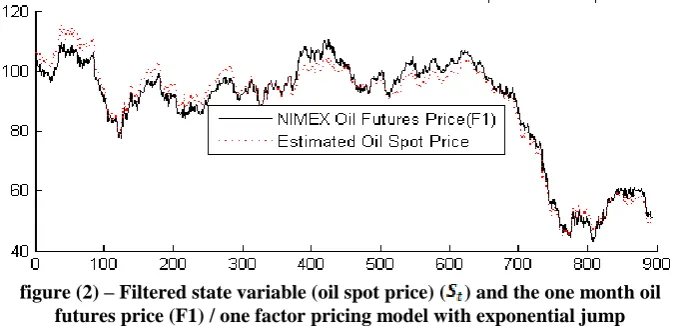
figure (2) – Filtered state variable (oil spot price) ( ) and the one month oil futures price (F1) / one factor pricing model with exponential jump
Source: The research findings
Due to decline in oil prices in 2015 is expected that decreasing jump of the model be significant. While the one factor model with exponential jumps has a zero estimate for this parameter. On the other hand, increasing jump amplitude shows 37% change in the log spot price at the time of jump, that is not consistent with observations. So one factor model with exponential jump dose not improve the results of one factor model without jump and use of this model to pricing of NIMEX crude oil futures contract is not recommended.
significance level of 5 percent. According to these two parameters, log
price volatilities is estimated at around 0/12 in the diffusion section.
Reducing the value of this parameter in this model respect to the one factor model without jump, indicating absorption part of crude oil log spot price volatility by the jump component. The market value of risk per unit spot price estimated in the model also is not significant.
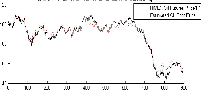
figure (3) – Filtered state variable (oil spot price) ( ) and the one month oil futures price (F1) / one factor pricing model with uniform jump
Source: The research findings
All three parameters of jump part, include rate of spot price jump number (η), the upper bound of jump amplitude (U) and the lower bound of jump amplitude (D) are statistically significant in this model. Based on the results, the rate of spot price jump number is 0/58. The upper bound of jump size is 0/36 which shows 8 percent change relative to the mean of closest maturity futures log price (16/13). Also the lower bound of jump size is -0/65 which shows 14 percent change in comparison with the mean of closest maturity futures log price.
In the figure (3), the time trend of the crude oil futures with the closest maturity (F1) and the state variable of oil spot price ( ) was plotted by using one factor futures pricing model with uniform jump.
5- Conclusions
Parts of the financial instruments that have a strong role in the development of the financial market are derivatives. Among the derivatives tools, futures contracts are one of the most important and repeatedly used in many financial markets all around the world.
Futures Pricing in contact play an important role in covering risk due to the nature of depending to the future of these contracts. In order to provide theoretical pricing models, futures one-factor pricing model of Ross (1995) and Schwartz (1997) have been used as a base model. Then, the base futures one factor pricing model of a commodity has been developed by adding jump to the dynamics of the spot price. To achieve this purpose, two futures one factor model of a commodity were extracted by using stochastic jump size with exponential distribution and stochastic jump size with uniform distribution.
Finally, all three futures one factor pricing model have been experimentally tested and compared by using the Kalman filter algorithm and NIMEX crude oil futures price data. Based on the results of one factor futures pricing model without jump, logarithm of the crude oil spot price followed the mean reversion process.
Logarithm of crude oil spot price in one factor futures model with exponential jump, such as no-jump model, followed mean reversion process in diffusion part. This result confirmed one factor no-jump model. But this model did not have good performance in the jump component of crude oil spot price. However, decreasing jump of the model is expected due to the decline of crude oil price in 2015. While the one factor model with exponential jumps has been estimated zero . So one factor model with exponential jump did not improve the results of one factor model without jump and use of this model to pricing of NIMEX crude oil futures contract is not recommended.
comparison with one factor no-jump model gives more information about the oil price behavior. So, the use of this model is strongly recommended due to improved results compared to two other NIMEX crude oil futures pricing model . The estimated parameters in this model not only shows the dynamics of oil price, but also shows the not-continuity of oil price or existence of jump in oil price.
References
1- Bjerksund,P(1991). Contingent claims evaluation when the convenience yield is stochastic: Analytical Results. Working Paper, Norwegian School of Economics and Business Administration.
2- Bjork, Tomas(2003). Arbitrage Theory in Continuous Time
(2ndEdition). London :Oxford University Press.
3- Black, F. and M. Scholes (1973). The pricing of options and corporate liabilities. Journal of Political Economy, 81, 637–659.
4- Carmona Rene and Ludkovski Michael(2004). Spot Convenience Yield for the Energy Markets. Contemporary Mathematics, Volume 351
5- Cartea Alvaro and Figueroa Marcelo(2005). Pricing in Electricity Markets: A Mean Reverting Jump Diffusion Model with Seasonality. Applied Mathematical Finance, 12(4)
6- Dempster M.A.H and Medova Elena and Tang Ke (2015).Long and Short Term Jumps in Commodity Futures Prices.Working Paper, Centre for Financial Research, Judge of Business School
7- Duffie, D., J. Pan and K. Singleton, (2000). Transform analysis and asset pricing for affine jump diffusions. Econometrica 68, pp1343-1376. 8- Esposito, Elena (2011). The Future of Futures. Cheltenham, UK. Northampton, MA, USA. Edward Elgar Publishing
9- Harvey Andrew C(1991). Forecasting, Structural Time Series Models and the Kalman Filter. Cambridge University Press
10- Hull, John c (2012). Options,Futures and Other Derivatives
(8thEdition). Canada, Prentice Hall.
11- Lee, Kai Ming (2010). Filtering Non-Linear State Space Models: Methods and Economic Applications. Issue 474 of Tinbergen Institute research series. ozenberg Publishers
12- Martin Matthew Stephen(2007). A Two-Asset Jump Diffusion Model with Correlation. A thesis submitted for the degree of MSc Mathematical Modelling and Scientific Computing. University of Oxford. Exeter College.
13- McDonald Robert (2006). Derivatives Markets (2nd Edition). USA,
Addison Wesley.
16- Mikosck, Tomas(2000). Elementary Stochastic Calculus.Singapore, London, World Scientific.
17- Ross, S.A(1995). Hedging long run commitments: exercises in incomplete market pricing.Preliminary Draft.
18- Schwartz, E. S(1997). The stochastic behavior of commodity prices: implications for valuation and hedging. The Journal of Finance, LII. No.3, PP.922-973.
19- Schwartz, E. Sand Smith, James E (2000).Short-term variations and long-term dynamics in commodity prices.Management Science, Vol.46, No.7, PP. 893-911.
20- Tankov Peter and Cont Rama(2004). Financial Modelling With Jump Processes. USA. Chapman & Hall/CRC
21- Villaplana Pablo(2003). Pricing Power Derivatives: A Two-Factor Jump-Diffusion Approach. Working Paper. Business Economics Series 05. Universidad Carlos III de Madrid