Neural-network based vector control of VSCHVDC transmission systems

      

City, University of London Institutional Repository

Citation

:

Li, S., Fu, X., Alonso, E., Fairbank, M. and Wunsch, D. C. (2016).

Neural-network based vector control of VSCHVDC transmission systems. Paper presented at the

4th International Conference on Renewable Energy Research and Applications (ICRERA),

22-25 Nov 2015, Palermo, Italy.

This is the accepted version of the paper.

This version of the publication may differ from the final published

version.

Permanent repository link:

http://openaccess.city.ac.uk/14793/

Link to published version

:

http://dx.doi.org/10.1109/ICRERA.2015.7418673

Copyright and reuse:

City Research Online aims to make research

outputs of City, University of London available to a wider audience.

Copyright and Moral Rights remain with the author(s) and/or copyright

holders. URLs from City Research Online may be freely distributed and

linked to.

City Research Online:

http://openaccess.city.ac.uk/

[email protected]

Abstract—The application of high-voltage dc (HVDC) using voltage-source converters (VSC) has surged recently in electric power transmission and distribution systems. An optimal vector control of a VSC-HVDC system which uses an artificial neural network to implement an approximate dynamic programming algorithm and is trained with Levenberg-Marquardt is introduced in this paper. The proposed neural network vector control algorithm is analyzed in comparison with standard vector control methods for various HVDC control requirements, including dc voltage, active and reactive power control, and ac system voltage support. Assessment of the resulting closed-loop control shows that the neural network vector control approach has superior performance and works efficiently within and beyond the constraints of the HVDC system, for instance, converter rated power and saturation of PWM modulation.

Keywords—VSC-HVDC transmission and distribution; renewable energies; neural network; adaptive dynamic programming; Levenberg-Marquardt, voltage-source converter

I. INTRODUCTION

VSC-HVDC relies on voltage source converters (VSCs) and insulated gate bipolar transistors (IGBT) [1] for the transmission and distribution of energy. VSC-HVDC shows distinct advantages, namely: low cost, small environmental footprint, easy integration of renewables to the transmission grid, and high transmission stability and power quality [2].

Since HVDC transmission using VSC was first installed in 1997 in Gotland (Sweden) [3], two main manufacturers refer to the technology of HVDC transmission using VSCs, namely, ABB under the name of HVDC Light [3], with a power rating from tenths of megawatts up to over 1000 MW, and Siemens under the name of HVDC Plus ("Plus" - Power Link Universal Systems) [4]. VSC-HVDC technology has been broadly applied

This paper has been partly financed by the U.S. NSF Grant EECS 1102038/1102159, the Mary K. Finley Missouri Endowment, and the Missouri S&T Intelligent Systems Center.

in microgrids and in integration of solar and offshore wind into the power transmission system [5, 6].

Typically, a VSC-HVDC system is controlled via a nested-loop control, which in turn is built on standard vector control methods [5-7]. However, recent studies show that a complete decoupled vector control cannot be achieved using conventional methods, which affects the performance of the standard vector control method, particularly if a converter works beyond the PWM (pulse-width-modulation) saturation bound [8].

It has also been indicated that there are unresolved challenges which prevented effective integration of offshore wind to the grid using HVDC [9]. It has been shown, on the other hand, that an optimal vector control of a grid-connected converter can be approximated by using an artificial neural network [10].

In this paper, a neural network control technique based on approximate dynamic programming principles which meets various HVDC control requirements is presented. The paper makes the following new contributions:

1) a neural network control strategy for VSC-HVDC

systems

2) neural network design and training that can handle

VSC-HVDC control requirements properly under physical system constraints, and

3) comparison of standard and neural network control

methods for power control and management of a HVDC transmission system.

With this aim in mind, we first specify the configuration of a VSC-HVDC system in the next section. Section III shows both the standard and a novel neural network vector control topologies for HVDC inverter and rectifier stations. The training of the neural network vector controller is discussed in Section IV. Performance of a VSC-HVDC system by using the conventional and neural network vector control methods is discussed in Sections V for different HVDC operating conditions. We shall finish with conclusions.

Neural-Network Based Vector Control of

VSC-HVDC Transmission Systems

Shuhui Li, Xingang Fu

The University of

Alabama Tuscaloosa AL, USA

Eduardo Alonso

City University London

London, UK

Michael Fairbank

University of Essex

Colchester, UK

Donald C. Wunsch

Missouri Univ. of Sc. and Tech.

Transmission line

Transmission line

Transmission line

Transmission line Phase reactor

AC filters AC

system 1 Phase reactor

AC filters

AC system 2

[image:3.612.47.563.56.195.2]

VSC Station 1 VSC Station 2

Fig. 1. Configuration of a two-terminal VSC-HVDC transmission system

II. CONTROL OF VSC-HVDCSYSTEM

A. VSC-HVDC Transmission

Transmission in VSC-HVDC involves VSC-based converter stations and a high-voltage dc transmission system [5, 6].

The stations need to efficiently regulate their reactive power or ac system voltage support control and their active power or dc system voltage control [11]. While each of the converter stations controls its reactive power independently, the active power entering the HVDC system must be equal to the resultant active power leaving it [12].

In the HVDC system, one station is built to control the voltage of the dc system where as the other VSC stations control the active power.

[image:3.612.52.297.476.575.2]

Figure 1 shows a schematic a VSC-HVDC system with two stations. The stations are connected to an ac system via a phase reactor and a transformer. An ac filter is used on each side of the ac system to reduce or eliminate the harmonics entering the ac systems. Regarding dc, the stations are connected to a capacitor bank. Stations work as a rectifier and an inverter respectively.

Fig. 2. Design of a VSC station

B. VSC Station Model in d-q

Figure 2 details how a VSC station is connected to an ac system, in which a capacitor is connected across the dc side of the VSC, the composition of a resistor R and an inductor L represents the phase reactor, and a three-phase voltage source stands for the voltage at the Point of Common Coupling (PCC). In the d-q reference frame [7, 8], the VSC-HVDC system is represented by

1

1

1 1

d s d d d

q s q q q

i R L i v v

d

i R L i v v

dt L L

ω

ω

−

⎡ ⎤₌₋⎡ ⎤⎡ ⎤₋ ⎡ ⎤₊ ⎡ ⎤

⎢ ⎥ ⎢ ⎥⎢ ⎥ ⎢ ⎥ ⎢ ⎥

⎣ ⎦

⎣ ⎦ ⎣ ⎦ ⎣ ⎦ ⎣ ⎦ (1)

where ωs is the angular frequency of the ac system voltages and the rest of the symbols in Eq. (1) are consistent with those indicated in Fig. 2, e.g., va,vb,vc↔vd,vq; ia,ib,ic↔id,iq; and va1,vb1,vc1↔vd1,vq1.

C. Vector Control of VSC Stations

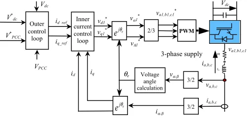
The general VSC vector control method deploys a nested-loop structure with inner and outer current nested-loops, the former being faster than the latter, as shown in Fig. 3 [5, 13]. Active power or dc voltage is controlled through the d-axis loop, whereas, the q-axis loop controls the reactive power or PCC voltage.

The power controllers generate d- and q-axis references to the inner current-loop controller where as the inner controller applies a three-phase sinusoidal voltage signal directly to the VSC converter [5].

The overall strategy for the conversion of d-q signals into three-phase sinusoidal signals is illustrated in Fig. 3, in which vd1* and vq1* are d- and q-axis output voltages.

The d- and q-axis voltages are transformed to the three-phase sinusoidal voltage signals, va1*, vb1* and vc1*, through Park transformation [8].

Fig. 3 Common vector control structure of HVDC VSC PWM

3/2 2/3

va1,b1,c1*

vα,β vα1*

vβ1* vd1* id_ref

Vdc

va,b,c e

j

eθ

iq_ref

vq1*

3/2 iα,β

ia,b,c

e

j

eθ Inner current control loop

id iq

va1,b1,c1

Voltage angle calculation

ia,b,c θe

V* dc

Vdc

V* PCC

VPCC Outer control loop

3-phase supply R L ia

ib

ic

va

vb

vc

va1

vb1

[image:3.612.314.565.523.644.2]

III. STANDARD AND NEURAL NETWORK CONTROL

STRUCTURES

A. Conventional Standard Vector Controller

Figure 4 shows the standard vector control structure as applied to a VSC [5, 13]. Since the absolute decoupling between d- and q-axis loops is impossible, the conventional vector control has a competing control nature [8], which may derogate the controller or system performance (see the evaluation shown in Section V). The design of the inner current-loop controller results from editing Eq. (1) as

(

)

1

d d d s q d

v = R i⋅ +L di dt⋅ −

ω

L i⋅ +v (2)

(

)

1

q q q s d

v = R i⋅ +L di dt⋅ +ωL i⋅ (3)

[image:4.612.57.305.286.365.2]

where the bracketed term of (2) and (3) represents the state equation between the voltage and current on d- and q-axis loops; the rest are compensation terms [14, 15].

Fig. 4. Conventional standard vector control structure

There are a number of items that need to be analyzed in the conventional vector control design:

1) To avoid that the VSC exceeds the PWM saturation limit, Eq. (4) is used [16], where vd1_new* and vq1_new* are the modified controller d- and q-axis voltages, and Vmax is the maximum allowable dq voltage.

(

)

(

)

* * * *

1_ max_

cos

1 1_ max_

sin

1

d new GSC dq q new GSC dq

v

=

V

∠

v

v

=

V

∠

v

(4)

2) To avoid that the VSC exceeds the rated current limit, Eq. (5) is used, i.e., a strategy to keep the d-axis current reference id* constant to retain active power or dc-link voltage control

effectiveness where as changing the q-axis current reference iq* to meet the requirements of the support control [16].

( ) (

) ( )

2 2

* * * * * *

_ _ sign _ max

d new d q new q dq d

i =i i = i ⋅ i − i (5)

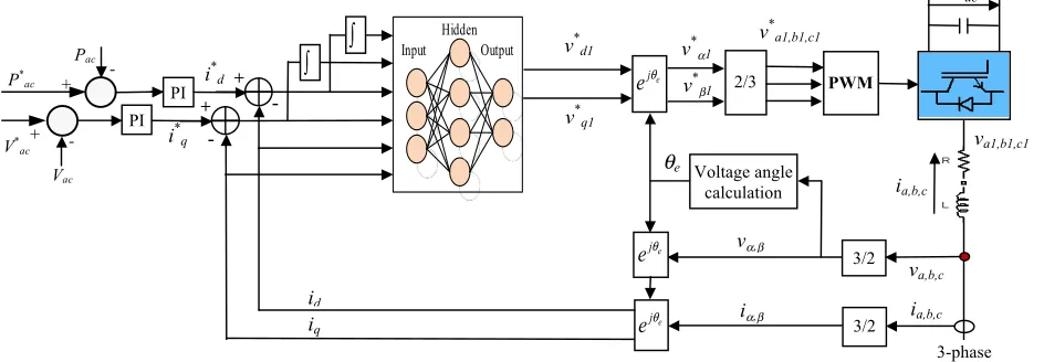
B. Neural Network Vector Controller

The neural-network vector control architecture of a VSC is shown by Fig. 5. The neural network implements the fast inner current loop control function.

Unlike a conventional PI-based controller, the neural network is trained to approximate optimal control. The neural network, a.k.a. the action network, is applied to the VSC through a PWM mechanism to regulate the converter output voltage va1,b1,c1 in the three-phase ac system (Fig. 3). The ratio of the output voltage added by a VSC to the output of the action neural network is a boost of kPWM, Vdc/2 if the amplitude of the triangle voltage waveform is 1V [17].

For digital control implementation using an artificial neural network, the system as given by Eq. (1) is converted to the discrete state-space model in Eq. (6) [18], where Ts represents the sampling period,kis a time step, and F and G are the system matrix and the control matrix respectively.

The discrete system model in Eq. (6) can be rewritten in the vector way as shown by Eqs. (7) to (9).

(

)

(

)

( )

( )

11

( )

( )

d s s d s d s d

q s s q s q s q

i kT T i kT v kT v

i kT T i kT v kT v

+ −

⎡ ⎤ ⎡ ⎤ ⎡ ⎤

= +

⎢ ₊ ⎥ ⎢ ⎥ ⎢ ₋ ⎥

⎣ ⎦ F⎣ ⎦ G⎣ ⎦

(6)

i!"!_dq(k+1)=F⋅i!"!_dq(k)+G⋅u! "!_dq(k) (7)

u

_dq

! "

!

(

k

)

=

v

! "

!!

_dq1

(

k

)

−

v

! "

!

_dq (8)

v_dq1

! "!!

(k)=k_PWMA

(

"i_dq

( )

k ,! "e!_dq

( )

k ,s! "!_dq

( )

k ,w"

)

(9)

The action neural network is a fully connected multi-layer perceptron and makes the control decision A

(

!i_dq,e" !"_dq," !"s_dq,w!

)

at

PI

V* dc

Vdc

+

- _i*

d

|idq|

Limiter eq. (5)

PI

id

+ -

|vdq|

Limiter eq. (4)

v’ d

- ωsL⋅iq

+ v*

d1 v*d1_new

PI

V* bus

Vbus

+

- _i*

q

PI

iq

+

- _v’

q - ωsL⋅id

- v*

q1 v*q1_new vd

+

PWM

3/2

3-phase supply 2/3

-

+

v* a1,b1,c1

vα,β

v*

α1 v*β1 i*

d

Vdc

va,b,c

e j eθ

-

+

i* q

3/2

iα,β ia,b,c

e j eθ

id iq

va1,b1,c1

∫

∫

Voltage angle calculation

Fig. 5. Neural network vector control architecture of a VSC-HVDC converter station

ia,b,c

θe v*d1

v* q1

e

j eθ

PI

P* ac

Pac +

-PI

V*

ac

-+

Vac

Input Hidden

[image:4.612.327.552.343.443.2] [image:4.612.77.549.532.696.2]

each time step k in Eq. (9), where

!

i

_dqrepresents actual dq

current vector of ac system, and

e

! "

_dq

!

and

s

! "!

_dq represent error current and integral of the error current as shown in Fig. 5. The integral term can help to remove the steady error and to maintain the stable operation of the converter when the converter has a potential to go over the PWM saturation limit. This is analyzed in Section V-B.

IV. DETERMINE CONTROLLER PARAMETERS

A. Tuning PI Parameters of Standard Vector Controller The tuning of the conventional current-loop PI controller is based on Fig. 6. Here, the PI block stands for a d- or q-axis loop current controller, and 1/(L⋅s+R) represents the plant transfer function for a d-or q-axis current loop (Eqs. (2) and (3)) [8, 19, 20]. kFB_I is the gain of the feedback path, for example, then gain of a current sensor; and kPWM is the gain of the power electronic converter. Based on Fig. 6, the best possible gain of the PI controller can be tuned conveniently with Matlab Simulink. However, there are only two parameters that can be tuned for each PI controller.

Fig. 6. A system block diagram for design of current-loop PI controller

B. Training Neural Network Vector Controller

The neural-network vector controller was trained using dynamic programming (DP) principles, aiming to approximate optimal control. DP employs Bellman’s Principle of Optimality [21, 22, 23]. The typical structure of a discrete-time DP problem includes a performance index, or cost function, and a discrete-time system mode [23]. The DP cost function which we used for this VSC vector-control problem was defined as:

C i

(

!"!_dq

( )

j ,w"

)

= γk−j_U(e dq

! "!

(k)) k=j

∞

∑

,j>0,0<γ ≤1 (10)

where γ is a constant referred to as the discount factor, and U is defined as:

U(e! "_dq!(k))= e_d2_(k)+e q 2_(k)

⎡⎣ ⎤⎦α

=

{

⎡⎣i_d(k)−i_{d_ref}(k)⎤⎦2+⎡⎣i_q(k)−i_{q_ref}(k)⎤⎦2

}

α,α>0

(11)

and where α is a constant. The function C(⋅) is referred to as the cost-to-go function from the given state i!"!_dq(j) and time

step j of the DP problem. The objective of the neural network

controller is to track a reference current trajectory in an optimal manner, i.e., to hold the actual state !i_dqnear a target

state!i_dq* _{so that the function C(⋅) in Eq. (10) is minimized. The}

neural network was trained by using Levenberg-Marquardt (LM) [24] to minimize the DP cost C(⋅). We chose the LM algorithm because it is particularly suited to situations in which the model functions are known and differentiable, and because it is the fastest neural network training algorithm for a moderate number of network parameters. The use of LM requires a modification of the cost function C(⋅) defined in Eq.

(10), as follows: Consider the cost function

C= γk−j_U(e dq

! "!

(k)) k=j

N

∑

withγ =1, j=1, and k=1, , .K N _Then,

we rewrite C(⋅) as:

C= U(e! "!_dq(k))

k=1

N

∑

=

( )

V(k)2

k=1

N

∑

(12)

where we define V(k)= U(e! "_dq!(k)) . Now, we can derive the

gradient

∂

C

/

∂

w

!"

as:

∂C ∂w!"=

∂

(

V(k)

)

2

k=1

N

∑

∂w!" = 2V(k) ∂V(k)

∂!"w

k=1

N

∑

=2J(w!")T_V!"

(13) where the Jacobian matrix

_J

(

w

!"

)

is:

J(!"w)=

∂V(1)

∂w₁ #

∂V(1)

∂w_M

$ % $

∂V(N)

∂w₁ #

∂V(N)

∂w_M ⎡

⎣ ⎢ ⎢ ⎢ ⎢ ⎢ ⎢

⎤

⎦ ⎥ ⎥ ⎥ ⎥ ⎥ ⎥

, V!"= V(1)

$

V(N)

⎡

⎣ ⎢ ⎢ ⎢

⎤

⎦ ⎥ ⎥ ⎥

(14)

Then, the process of updating the weights using LM [24] for the neural network controller can be expressed as:

Δw!"=− J(w!")T

J(w!")+

µI

⎡

⎣ ⎤⎦

−1

J(w!")T V!"

(15)

The parameter µ was adjusted dynamically during training,

so as to ensure that cost function always decreased. In order to increase the speed of computation, the weights update in Eq. (15) was conducted using Cholesky factorization [25]. To train the action network, the system data associated with Eq. (1) such as R, L, vd, and vq were specified. Before training, the weights of the neural network were randomized with a Gaussian distribution of mean zero and variance 0.1. The training procedure for the current-loop action network

involved: 1) randomly generating a sample initial state i!"!_dq(1);

[image:6.612.53.566.52.144.2]

Fig. 7. A VSC-HVDC system with feedback control built in MATLAB SimPowerSystems and RT-LAB

PWM saturation and the impact of variable phase reactor values. This training process resulted in a neural network

capable of handling VSC control, under the distorted or

imbalanced PCC voltage conditions and short circuits in ac or dc system, as described further in Section V-C.

V. RESULTS

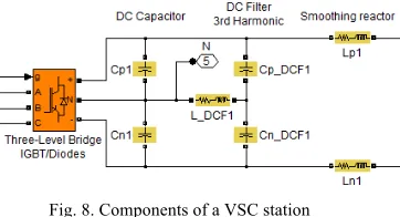
[image:6.612.84.265.416.514.2]

In order to assess the performance of the conventional and neural network methods, we developed a VSC-HVDC system in SimPowerSystems (Fig. 7) (parameters in Appendices). A three-level neutral-point-clamped VSC was adopted in order to guarantee power quality at the stations [26]. Each VSC station includes a phase reactor and ac filters on the ac system side and capacitors, filters and smoothing reactors on the dc system side as shown by Fig. 8. The parameters of a VSC station are given in Table 2. The PI gains of outer-loop controllers and inner current-loop controllers of the conventional method are given in Table 3. Major measurements include voltages, currents, and active and reactive powers at PCC1 and PCC2, and dc capacitor voltages.

Fig. 8. Components of a VSC station

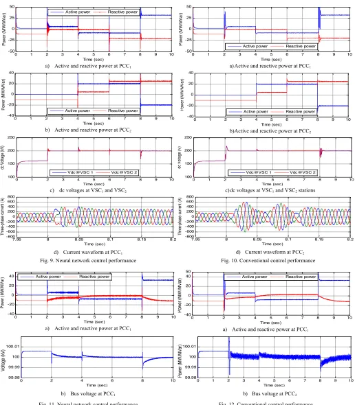
A. Control of Power Transmission between VSC Stations Figures 9 and 10 compare the performance of the HVDC system utilizing both control approaches. At the beginning, the two breakers are in open position and the dc transmission lines are charged to 168kV by ac system 1 through the resistor in parallel with Breaker 1 and the inherent diodes in parallel with the IGBT switches of VSC station 1. After Breaker 1 is closed at t=2s, the dc voltage is regulated quickly to 200kV, the reference value, using the neural network vector controller (Fig. 9c) without a high over current (Fig. 9d). At t=4s, Breaker 2 is closed and a 20MW is delivered to ac system 1 from ac system 2, which causes the dc system voltage to increase. With the neural network controller, the dc system voltage is quickly stabilized at 200kV. At t=8s, the power demand at the VSC-station 2 changes requiring 20MW from ac system 1, resulting in a high dc voltage drop. But, the neural network controller rapidly stabilizes the dc voltage. For

all the other conditions, the neural network controller shows a fast response speed with low current and voltage oscillations. The standard vector controller shows similar performance for power transmission control between the two VSC stations (Fig. 10). Compared to the neural network vector controller, the standard vector controller shows higher oscillations (Figs. 9c and 10c, Figs. 9d and 10d). This is due to the fact that the control action generated by the standard PI controller is determined by the error between the control parameter and the corresponding reference value. Hence, there must be overshoot and settling time issues associated with a PI-based controller. However, the neural network controller is designed and trained based on the DP-based optimal control principle. For an ideal optimal controller, a reference command can be reached immediately without any delay and overshoot. But, this cannot be achieved practically because of physical system constraints. The neural network controller tries to approximate an ideal optimal controller within the physical system constraints. Therefore, the neural network controller has the advantages for fast power transmission control between VSC stations with small oscillations as shown by Figs. 9 and 10.

B. Power Transmission and PCC Voltage Control

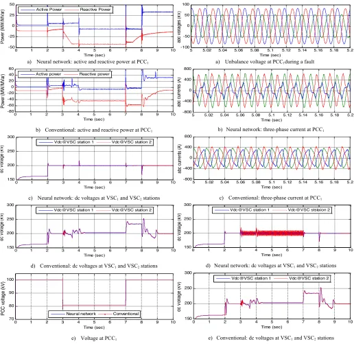
Now the d-axis loop is employed for active power control while the q-axis loop for PCC voltage control. Figs. 11 and 12 show how the neural network and conventional standard vector controllers perform under normal operating condition; Fig. 13, on the other hand, contrasts the activity of the neural network and conventional controllers under a fault in ac system 1 that appears between 3sec and 7sec. The active power condition is the same as that used in Figs. 9 and 10. For normal operating condition, the neural network and standard controllers perform similarly. However, under the faulted condition, a high reactive power is necessary to rise the PCC voltage, which may cause the converter exceed its PWM saturation limit.

Under the faulted condition, the standard vector controller enters into a malfunction state (Fig. 13d). This is because standard control methods are inherently competing (Section II-A). As a result, when the PWM saturation limit is surpassed, the competing control balance is affected and the control stability of d- and/or q-axis loop could lose. A typical approach to prevent the malfunction of the standard controller is to set a limit on the highest generating reactive power that is allowed. However, the actual real-time reactive power limit is

a) Active and reactive power at PCC1 a)Active and reactive power at PCC1

b) Active and reactive power at PCC2 b)Active and reactive power at PCC2

c) dc voltages at VSC1 and VSC2

d) Current waveform at PCC1

c)dc voltages at VSC1 and VSC2 stations

d) Current waveform at PCC2

Fig. 9. Neural network control performance Fig. 10. Conventional control performance

a) Active and reactive power at PCC1 a) Active and reactive power at PCC1

[image:7.612.49.565.45.635.2]

b) Bus voltage at PCC1

Fig. 11. Neural network control performance

b) Bus voltage at PCC2

Fig. 12. Conventional control performance

voltage etc, which causes a challenge to the conventional standard vector controller.

For the neural network controller, the sigmoid function of the network automatically turns the d-axis voltage of the controller into saturation when the PWM saturation appears due to the need of large reactive power. Thus, such power is locked at the maximum generating reactive power according to real-time condition for the highest possible PCC voltage

support control (Fig. 13a) while the control of the active power or dc voltage still keeps the normal control mode (Fig. 13c), which overcomes the challenge of the standard controller and improves VSC-HVDC reliability and stability.

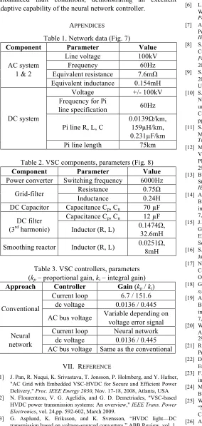
C. Control under Unbalanced Fault

An unbalanced fault is caused by either one-phase or two-phase short circuit in an ac power system. Fig. 14 compares

0 1 2 3 4 5 6 7 8 9 10

-50 -25 0 25 50 Po w er ( M W /M Va r) Time (sec)

Active power Reactive power

0 1 2 3 4 5 6 7 8 9 10

-50 -25 0 25 50 Po w er ( M W /M Va r) Time (sec)

Active power Reactive power

0 1 2 3 4 5 6 7 8 9 10

-40 -20 0 20 40 Po w er ( M W /M Va r) Time (sec)

Active power Reactive power

0 1 2 3 4 5 6 7 8 9 10

-40 -20 0 20 40 Po w er ( M W /M Va r) Time (sec)

Active power Reactive power

0 1 2 3 4 5 6 7 8 9 10

100 150 200 250 dc V ol ta ge ( kV ) Time (sec)

Vdc@VSC 1 Vdc@VSC 2

7.95 8 8.05 8.1 8.15 8.2

-800 -600 -400 -200 0 200 400 600 800 Th re e-ph ase c ur re nt ( A) Time (sec)

0 1 2 3 4 5 6 7 8 9 10

100 150 200 250 dc V ol tage ( V ) Time (sec)

Vdc@VSC 1 Vdc@VSC 2

7.95 8 8.05 8.1 8.15 8.2

-800 -600 -400 -200 0 200 400 600 800 Th re e-ph ase c ur re nt ( A) Time (sec)

0 1 2 3 4 5 6 7 8 9 10

-40 -20 0 20 40 Po w er ( M W /M Va r) Time (sec) Active power Reactive power

0 1 2 3 4 5 6 7 8 9 10

-40 -20 0 20 40 50 Po we r (MW /MV ar) Time (sec)

Active power Reactive power

0 2 4 6 8 10

99.98 99.99 100 100.01 Vo lta ge (k V) Time (sec)

0 1 2 3 4 5 6 7 8 9 10

a) Neural network: active and reactive power at PCC1

b) Conventional: active and reactive power at PCC1

c) Neural network: dc voltages at VSC1 and VSC2 stations

d) Conventional: dc voltages at VSC1 and VSC2 stations

e) Voltage at PCC1

a) Unbalance voltage at PCC1during a fault

b) Neural network: three-phase current at PCC1

c) Conventional: three-phase current at PCC1

d) Neural network: dc voltages at VSC1 and VSC2 stations

[image:8.612.49.565.48.549.2]

e) Conventional: dc voltages at VSC1 and VSC2 stations

Fig. 13. Performance evaluation under a balanced fault in ac system Fig. 14. Performance evaluation under an imbalanced fault in ac system

the performance of the neural network and standard

controllers under a one-phase fault appeared at PCC1 between

3sec and 7se. All the other conditions remain the same as those used in Fig. 13. The unbalanced fault made the control of VSC-HVDC more challenging. Both neural network and conventional controllers show oscillation during the fault period. Similar to Fig. 13, the standard controller could lose stability while the neural network controller is stable during the unbalanced fault conditions, demonstrating a good adaptive capability

VI. CONCLUSIONS

In this paper, a neural network vector control mechanism is presented and compared with the standard vector control

method for VSC-HVDC control. The neural network controller is trained based on dynamic programming to approximate the optimal control while the standard controller is based on the PI control principle. The neural network controller shows a smaller overshoot and responds faster compared to the conventional controller.

In the PCC voltage support control mode, the conventional standard controller may enter into a malfunction state especially under a high voltage drop at the PCC bus, which may affect the stable operation of the HVDC system. The neural network controller can overcome this limitation by achieving the highest possible PCC voltage support control while the control of the active power or dc voltage is not affected.

0 1 2 3 4 5 6 7 8 9 10

-50 -25 0 25 50

Po

we

r (MW

/MV

ar)

Time (sec) Active Power Reactive Power

0 1 2 3 4 5 6 7 8 9 10

-80 -60 -40 -20 0 20 40 60

Po

we

r (MW

/MV

ar)

Time (sec) Active power Reactive power

0 1 2 3 4 5 6 7 8 9 10

150 200 250 300

dc

V

olta

ge

(kV

)

Time (sec)

Vdc@VSC station 1 Vdc@VSC station 2

0 1 2 3 4 5 6 7 8 9 10

150 200 250 300

dc

V

olta

ge

(kV

)

Time (sec)

Vdc@VSC station 1 Vdc@VSC station 2

0 1 2 3 4 5 6 7 8 9 10

70 80 90 100

PC

C v

olt

age

(kV

)

Time (sec)

Neural network Conventional

5 5.02 5.04 5.06 5.08 5.1 5.12 5.14 5.16 5.18 5.2 -100

-50 0 50 100

ab

c v

olta

ges

(kV

)

Time (sec)

5 5.02 5.04 5.06 5.08 5.1 5.12 5.14 5.16 5.18 5.2 -800

-400 0 400 800

ab

c c

urren

ts

(A)

Time (sec)

5 5.02 5.04 5.06 5.08 5.1 5.12 5.14 5.16 5.18 5.2 -800

-400 0 400 800

ab

c c

urren

ts

(A)

Time (sec)

0 1 2 3 4 5 6 7 8 9 10

150 200 250 300

dc

V

olta

ge

(kV

)

Time (sec)

Vdc@VSC station 1 Vdc@VSC ststaion 2

0 1 2 3 4 5 6 7 8 9 10

150 200 250 300

dc

V

olta

ge

(kV

)

Time (sec)

For an unbalanced fault in the ac system, both neural network and conventional controllers show oscillation during the fault period. The standard controller may lose stability while the neural network controller is stable even under the unbalanced fault conditions, demonstrating an excellent adaptive capability of the neural network controller.

[image:9.612.52.336.104.701.2]

APPENDICES

Table 1. Network data (Fig. 7)

Component Parameter Value

AC system 1 & 2

Line voltage 100kV

Frequency 60Hz

Equivalent resistance 7.6mΩ

Equivalent inductance 0.154mH

DC system

Voltage +/- 100kV

Frequency for Pi

line specification 60Hz

Pi line R, L, C

0.0139Ω/km,

159µH/km,

0.231µF/km

Pi line length 75km

Table 2. VSC components, parameters (Fig. 8)

Component Parameter Value

Power converter Switching frequency 6000Hz

Grid-filter Resistance 0.75Ω

Inductance 0.24H

DC Capacitor Capacitance Cp, Cn 70 µF

DC filter (3rd harmonic)

Capacitance Cp, Cn 12 µF

Inductor (R, L) 0.1474Ω,

32.6mH

Smoothing reactor Inductor (R, L) 0.0251Ω,

8mH

Table 3. VSC controllers, parameters (kp – proportional gain, ki – integral gain)

Approach Controller Gain (kp / ki)

Conventional

Current loop 6.7 / 151.6

dc voltage 0.0136 / 0.445

AC bus voltage Variable depending on

voltage error signal

Neural network

Current loop Neural network

dc voltage 0.0136 / 0.445

AC bus voltage Same as the conventional

VII. REFERENCE

[1] J. Pan, R. Nuqui, K. Srivastava, T. Jonsson, P. Holmberg, and Y. Hafner, "AC Grid with Embedded VSC-HVDC for Secure and Efficient Power Delivery," Proc. IEEE Energy 2030, Nov. 17-18, 2008, Atlanta, USA [2] N. Flourentzou, V. G. Agelidis, and G. D. Demetriades, "VSC-based

HVDC power transmission systems: An overview," IEEE Trans. Power Electronics, vol. 24,pp. 592-602, March 2009.

[3] G. Asplund, K. Eriksson, and K. Svensson, “HVDC light—DC transmission based on voltage-sourced converters,” ABB Review, vol. 1, pp. 4–9, 1998.

[4] K.Friedrich, "Modern HVDC PLUS application of VSC in Modular Multilevel Converter topology," Proc. 2010 IEEE International

Symposium on Industrial Electronics, pp. 3807 - 3810, July 4-7, 2010, Bari, Italy.

[5] P. Mitra, L. Zhang, and L. Harnefors, “Offshore Wind Integration to a Weak Grid by VSC-HVDC Links Using Power-Synchronization Control: A Case Study,” IEEE Trans. Power Del., vol. 29, no. 1, pp. 453-461, Feb. 2014.

[6] L. He, C. Liu, A. Pitto, and D. Cirio, “Distance Protection of AC Grid With HVDC-Connected Offshore Wind Generators,” IEEE Trans. Power Del., vol. 29, no. 2, pp. 493-501, Apr. 2014.

[7] A. Fuchs, M. Imhof, T. Demiray, and M. Morari, “Stabilization of Large Power Systems Using VSC–HVDC and Model Predictive Control,”

IEEE Trans. Power Del., vol. 29, no. 1, pp. 480-488, Feb. 2014. [8] S. Li, T.A. Haskew, Y. Hong, and L. Xu, “Direct-Current Vector

Control of Three-Phase Grid-Connected Rectifier-Inverter,” Electric Power System Research (Elsevier), Vol. 81, Issue 2, pp. 357-366, Feb. 2011.

[9] S. Saylors, "Advanced Wind Power Plant Solutions," Presented at 2014IEEE Power & Energy Society General Meeting, Washington DC, USA, July 27-31, 2014.

[10] S. Li, M. Fairbank, C.Johnson,D.C. Wunsch and E. Alonso, “Artifical Neural Networks for Control of a Grid-Connected Rectifier/Inverter under Disturbance, Dynamic and Power Converter Switching Conditions” IEEE Trans. Neural Netw.and Learn. Syst., Vol. 25, Issue 4, pp. 738-750, Apr. 2014.

[11] S. Mariéthoz, A. Fuchs, and M. Morari, “A VSC-HVDC Decentralized Model PredictiveControl Scheme for Fast Power Tracking,” IEEE Trans. Power Del., vol. 29, no. 1, pp. 462-471, Feb. 2014.

[12] Mats Hyttinen, Jan-OlofLamell, and Tom F Nestli, “New Application of Voltage Source Converter (VSC) HVDC to Be Installed on the Gas Platform Troll A,” Cigre 2004 Session Proceedings, Paris, France, Aug. 29 – Sep. 3, 2004,

[13] B. Silva, C.L. Moreira, H. Leite, and J.A. Peças Lopes, “Control Strategies for AC Fault Ride Through in Multiterminal HVDC Grids,”

IEEE Trans. Power Del., vol. 29, no. 1, pp. 395-405, Feb. 2014. [14] A. Luo, C. Tang, Z. Shuai, J. Tang, X. Xu, and D. Chen,

“Fuzzy-PI-Based Direct-Output-Voltage Control Strategy for the STATCOM Used in Utility Distribution Systems,” IEEE Trans. Ind. Electron., vol. 56, no. 7, pp. 2401-2411, July 2009.

[15] J.M. Carrasco, L.G. Franquelo, J.T. Bialasiewicz, E. Galván, R.C.P. Guisado, Ma.Á.M. Prats, J.I. León, and N. Moreno-Alfonso, “Power-Electronic Systems for the Grid Integration of Renewable Energy Sources: A Survey,” IEEE Trans. Ind. Electron., vol. 53, no. 4, 2006. [16] S. Casoria, “VSC-Based HVDC Transmission Link,” The MathWork,

January 2010.

[17] N. Mohan, T.M. Undeland, and W.P. Robbins, Power Electronics: Converters, Applications, and Design, 3rd Ed., John Wiley & Sons Inc., Oct. 2002.

[18] G.F. Franklin, J.D. Powell, M.L. Workman, Digital control of dynamic systems, 3rd edition, Addison-Wesley, 1998.

[19] A. Luo, C. Tang, Z. Shuai, J. Tang, X. Xu, and D. Chen, “Fuzzy-PI-Based Direct-Output-Voltage Control Strategy for the STATCOM Used in Utility Distribution Systems,” IEEE Trans. Ind. Electron., vol. 56, no. 7, pp. 2401-2411, July 2009.

[20] W. Wang, A.Beddard, M. Barnes, and O.Marjanovic, “Analysis of Active Power Control for VSC–HVDC,” IEEE Trans. Power Del., vol. 29, no. 4, pp. 1978-1988, Feb. 2014.

[21] R.E. Bellman, Dynamic Programming. Princeton, NJ: Princeton Univ. Press, 1957.

[22] D.E. Kirk, Optimal Control Theory: An Introduction, Prentice–Hall, Englewood Cliffs, NJ, Chaps. 1–3, 1970.

[23] F.Y. Wang, H. Zhang, and D. Liu, "Adaptive dynamic programming: An introduction," IEEE Comput. Intell. Mag., pp. 39–47, 2009.

[24] M. T. Hagan, H. B. Demuth and M. H. Beale, “Neural Network Design,” Boston: PWS, 2002, ch.12, pp 19-23.

[25] W. H.Press, B. P. Flannery, S. A. Teukolsky, and W. T. Vetterling, “Numerical Recipes in C: The Art of Scientific Computing (2nd Ed.),” Cambridge University Press, October 1992, pp. 994.