DEMOGRAPHIC RESEARCH
VOLUME 32, ARTICLE 55, PAGES 1487
−
1518
PUBLISHED 11 JUNE 2015
http://www.demographic-research.org/Volumes/Vol32/55/ DOI: 10.4054/DemRes.2015.32.55
Research Article
Long-term consequences of adolescent fertility:
The Colombian case
B. Piedad Urdinola
Carlos Ospino
©2015 B. Piedad Urdinola & Carlos Ospino.
This open-access work is published under the terms of the Creative Commons Attribution NonCommercial License 2.0 Germany, which permits use, reproduction & distribution in any medium for non-commercial purposes, provided the original author(s) and source are given credit.
1 Introduction 1488
2 Motivation 1490
3 Research strategy 1494
3.1 Pre-existent socioeconomic conditions 1500
3.2 The data 1503
3.3 Treatment and control groups 1505
4 Results 1505
4.1 Internal Validity Test 1508
5 Conclusions 1509
6 Acknowledgements 1511
Long-term consequences of adolescent fertility: The Colombian case
B. Piedad Urdinola1
Carlos Ospino2
Abstract
BACKGROUND
Estimating the long-term effects of adolescent motherhood is challenging for all developing countries, including Colombia, where this rate has been steadily increasing for 24 years, despite the reduction in the overall fertility rate. We propose a replicable methodology by applying a pseudo panel that evaluates the consequences of adolescent motherhood on outcomes previously neglected in the literature, such as job quality, marriage instability, partner’s job class, presence of physical abuse by current partner, and children’s health.
OBJECTIVE
To examine how adolescent mothers compare with non-adolescent mothers in outcomes not previously studied, such as job quality, marriage instability, partner’s job class, if respondent has been physically abused by current partner, and health outcomes for their children.
METHODS
We built a pseudo panel using four Demographic and Health Surveys (1995–2010) and compared the effects of older adolescent childbearing (ages 18–19) with those of women who postponed motherhood for just a couple of years (ages 20–21), exploiting the natural difference between adolescents and young adults who become mothers.
RESULTS
The results revealed younger mothers as well as their partners hold lower-class jobs, suffer higher rates of domestic violence at the hands of their partners, and have a higher share of deceased children.
1 Associate Professor, Department of Statistics, Universidad Nacional de Colombia-Bogotá, Colombia.
E-Mail: [email protected].
2 Ph.D. student, Department of Economics, Universidad de los Andes-Bogotá, Colombia.
CONCLUSIONS
The latter two results lead us to suggest aggressive and comprehensive targeted public policies both for prevention of adolescent motherhood and for following their just-born babies’ health.
1. Introduction
Although Colombia’s overall fertility rates have steadily declined since the 1960s, an unexpected rise in adolescent fertility has been observed during the past two decades. According to data from Demographic and Health Surveys (DHS) carried out in Colombia, age-specific fertility rates (ASFR) for females aged 15 to 19 have increased from 73.4 per thousand women in 1986 to 84 per thousand women in 2010. Interestingly, this increase has been observed in both rural and urban areas, among educated and uneducated females, and among married and unmarried women. It is thought that adolescents today have more options in life than did their counterparts in the past; the potential effects of adolescent childbearing on educational, employment, and marriage markets could thus be linked to the creation of cycles of poverty, while for older generations it was customary for Colombian women to marry as adolescents and soon become involved in motherhood.
There has been scant research on the long-term consequences of adolescent fertility in developing countries, partly due to the lack of available longitudinal data. Most studies have focused instead on the United States, where the adolescent fertility rate rose during the 1980s. Most of this research examined the educational and labor market outcomes of adolescent mothers, and found virtually no effect of adolescent motherhood on educational attainment but a positive effect on job enrollment, as adolescent mothers face additional pressures to find any work in order to provide for themselves and their child. However, the effects on long-term income and on child development are not so optimistic, with evidence suggesting lower socioeconomic status and lower educational attainment for children of adolescent mothers (Geronimus and Korenman 1992; Ermisch and Pevalin 2003; Hotz, McElroy and Sanders 2005).
The dearth of data available in developing countries, combined with the previous lack of attention paid to marriage market and health outcomes of adolescents’ children, have led us to examine the Colombian case, and to focus particularly on such consequences.3 Colombia has successfully collected six DHS from 1986 to 2010,
3 See TFR and ASFR built from Demographic and Health Surveys for Bolivia, Brazil, Colombia, the
allowing us to use the latest four to build a pseudo panel, a widely used statistical tool that compensates for the paucity of longitudinal data.4 We pooled birth cohorts of females born between 1964 and 1979, and followed through each DHS those women who bore their first child from ages 15 to 22, looking at their socio-economic outcomes by the age of 30 or above. Age 30 is desirable for the purpose of this study since the vast majority of Colombian women do not increase their educational levels after the age of 27 (less than 3%, according to DHS data), and 90% of women stop having children at age 29.
The use of a pseudo panel also allows us to correct for a problem typically encountered in cross-sectional data analysis, namely, results biased in the upward direction, as pointed out by experts in the Colombian case (Gaviria 2000; Núñez and Cuesta 2006). It also helps to reduce differences in family background and heterogeneity across a range of females who have babies at different ages, as average values are taken for all cohorts. However, the fact that it is not a real panel imposes challenges for the research question at hand. In particular, most studies suggest an association between higher adolescent fertility rates and low socioeconomic performances in the paternal household of adolescents (Azevedo et al. 2012; Lee 2010; di Cesare and Rodríguez 2006; Flórez Nieto 2005; Flórez Nieto et al. 2004; Geronimus, Korenman and Hillemeir 1994). To overcome this handicap, we proxy women’s paternal household socio-economic level with each woman’s height by the time of the survey.
Height, in adulthood, is a good proxy for paternal household’s socio-economic level, as argued by several authors in the demographic, economic (Fogel et al. 1982; Behrman and Hoddinot 2001; Alderman et al. 2006; Hatton 2013), and medical literature (Adair et al. 2013; Bhutta 2013; Brozek et al. 1977; Kulin et al. 1982; Morgane et al. 1993; Malcolm 1970; Habicht et al. 1974; Coly et al. 2006; Victora et al. 2008), because an adult’s height directly relates to nutritional intake during childhood. Thus, in both developed and developing countries, poorer households provide worse nutrition to their children than richer households, producing shorter adults.
Finally, it is difficult to isolate the pure effects of individual, familial, and environmental characteristics on the outcomes under study (see Lee 2010).5 We have found that in the vast literature on the study of the effects of adolescent motherhood one of the final challenges is identifying the appropriate contrast group for adolescents, regardless of the methodology. We believe that the closer the age to adolescence, the
4 DHS-1986 had a very different sampling design from the subsequent DHS surveys, as it was implemented
by an agency other than Profamilia (the Colombian agency in charge of survey fieldwork and processing since 1990). Also, DHS-1990 posed two problems for designing this study: it oversampled urban areas, as stated by Profamilia, and it produced very small-sized cells that did not provide the large numbers required for this research.
more appropriate the contrast will be. We choose, therefore, a quasi-experimental research design that sets treatment and control groups with an age difference of only one or two years, and at ages closer to the adolescent years (i.e., mothers ages 18–19 vs. mothers ages 20–21). We look at the outcomes when women are at least 30 years old at the time of the survey.
Our findings show that, after controlling for pre-existing socioeconomic status, compared to women giving birth at slightly later ages, younger mothers hold jobs of lower quality, their marriages or unions are more unstable, and, more importantly, partners tend to be more abusive when measured by domestic violence. Finally, significant detrimental effects are seen regarding the share of deceased children, an experience much more common for younger mothers. All of these effects reflect human capital losses that translate into poverty circles for these women and their children: cycles that need to be broken.
2. Motivation
Many Latin American countries (LAC) have recently experienced an unusual increase in adolescent fertility rates. Several studies have examined this phenomenon from different perspectives in the social sciences (Epidemiology, Economics, Demography, and Sociology). However, no papers focus on the long-term effects for these women on job quality, the stability of their personal lives, the probability of having an abusive partner, or their children’s health outcomes. We believe that, as in the American case, examination of the standard outcomes – years of education, employment status, and success in the marriage market – are limiting when measuring long-term effects of adolescent fertility, and might ultimately mislead policy implications.
We propose that it is very likely that long-term differences in educational attainment and employment rates between adolescent mothers and women who postponed maternity tend to disappear, because most of these young mothers come from socially challenged households and would probably achieve lower levels of these outcomes even if they were not adolescent mothers. Evidence from the United States and England during the 1980s corroborates this theory (Geronimus and Korenman 1992; Ermisch and Pevalin 2003; Hotz, McElroy, and Sanders 2005).6 Moreover, as most adolescent mothers were raised in households with lower socioeconomic conditions, there is an ongoing debate about the accountability of the full effects of
6 Note that short-term effects bias the long-term effects. In the American case the contrast of adolescent
adolescent fertility and educational outcomes, and about the causality between these events, as it directly relates to race and/or ethnicity in North America (Klepinger et al. 1995; 1999; Ribar 1994; Upchurch and McCarthy 1990).
For these reasons it is necessary to study outcomes that can actually capture the intensity of the effects for related variables when women are of an age when their educational attainment is unlikely to change drastically: we therefore chose to observe after age 29. In particular, we propose the measurement of job quality, to be defined and quantified as access to formal jobs. If adolescent mothers feel additional pressure to find work they are probably more prone to take any kind of job; the problem, therefore, is not the risk of unemployment but of taking lower-quality jobs, which could result in lower income later in life and, consequently, a reduced capacity to accumulate assets and savings.
LAC adolescent and unmarried mothers do not suffer from stigmatization in the marriage market, as they marry or live in consensual unions in similar proportions as women who delay motherhood (Buvinic 1998; Flórez Nieto and Núñez 2002). However, having a child is likely to be a less desirable trait in the marriage market, leaving adolescent mothers at risk of pairing up with lower-quality partners. We therefore propose to assess instability in the marriage market, as measured by having had more than one union. Partner quality is captured with two leading indicators: the job quality of the partner and the likelihood of the woman being abused by her current partner. For England and the United States there is evidence showing that mothers in their teens appear to fare worse in the marriage market, both in terms of the probability of getting married and the likelihood of partnering with men who become unemployed (Hotz et al. 1997; Ermisch and Pevalin 2003). By contrast, experiences from Barbados, Chile, Guatemala, and Mexico (Buvinic 1998), as well as Bolivia, Brazil, Colombia, the Dominican Republic, Guatemala, and Peru (Flórez Nieto and Núñez 2002) show that adolescent mothers do not have a lower probability of marrying, but do have a higher probability of having non-traditional family arrangements: more adolescent mothers as boarders; fewer biological fathers as heads of family (both in terms of assuming financial obligation for and in forming attachments to their children); and more grandparents taking over responsibility for children.
lower scores in Apgar test #1) for babies born to adolescent mothers, but at the same time these negative health associations are also linked to low socioeconomic strata across all Latin American hospitals, and are driven by a higher incidence among adolescent mothers of anemia, malnutrition, and less frequent prenatal and pediatric visits. These clinical studies also show that adolescent mothers in LAC have lower grades in school and unstable relationships that last no more than a year (Sánchez et al. 2006; Auchter et al. 2005; Perdomo et al. 2005; Fernández et al. 2004; Burgos and Carreño 1997). A recent study in different LAC supports this idea by presenting negative correlations between adolescent motherhood and maternal mortality, miscarriages, suicide, and infant mortality (Azevedo et al. 2012).
It is important to acknowledge that the results of clinical studies cannot be generalized; to achieve such generalizability a different kind of data is needed for analysis. By investigating the share of deceased children per woman we seek to fill this knowledge gap for LAC from a social sciences perspective. Through the use of a larger sample we hope to provide richer information than most case-clinical studies, thereby allowing for the control of other socioeconomic characteristics.
To put the Colombian case in perspective, it is important to remember that Colombia experienced a swift demographic transition, beginning with mortality in the 1950s when women, on average, had more than seven children during their reproductive years, and at the same time large investments in health and infrastructure were being made throughout the country. By the mid-1970s fertility reduction began, accompanied by a large wave of rural-urban migration, massive entry of women into the formal educational system and job market, and expansion of access to contraception. As a result the average number of children a Colombian woman had dropped from 4.7 in 1975 to 3.2 children in 1986 (Miller 2010; Flórez Nieto 2000). Throughout this process of demographic transition, fertility declined for women of all ages. However, the adolescent fertility rate (ages 15 to 19) has risen since 1986, while the total fertility rate (TFR) has continued to decrease in Colombia, along with all other age-specific fertility rates (ASFR), as depicted in Figure 1.
Figure 1: Age-Specific Fertility Rates (ASFR) by five-year age group in Colombia, 1986–2010
Source: www.statcompiler.com from Colombian-DHS for each year. (Downloaded September 25, 2013)
In the literature for all of these cases, most authors concur that this increase in adolescent fertility correlates with poverty (Lee 2010). In the Latin American context it also relates to lower educational levels (Azevedo et al. 2012; Rodríguez 2008), which in the Colombian case translates into girls’ low expectations for social mobility (Gavira 2000; Flórez Nieto et al. 2004; Flórez Nieto 2005; Azevedo et al. 2012) and increased likelihood of broken families or households where mothers of adolescents are absent, increasing the risk of adolescent motherhood (Flórez Nieto 2005).
Due to the limitations of the data, the consensus regarding studies carried out in Latin America is that cross-sectional data up-bias the results; in order to overcome this handicap most researchers have used statistical approaches as solutions: instrumental variables, Oaxaca-Blinder estimations, etc. With such constraints in mind, Colombian studies have found lower average education and job market outcomes for adolescent mothers than for their older counterparts; however, these results are positively correlated with the formation of unstable families, which in turn are associated with poverty (Núñez and Cuesta 2006; Gaviria 2000; Barrera and Higuera 2004). Similar evidence has been found for Uruguay (Gerstenblüth et al. 2009), Brazil (Berquo and
0 20 40 60 80 100 120 140 160 180 200
1986 1990 1995 2000 2005 2010
Cavenaghi 2005), and other LAC such as Mexico, Peru, and Ecuador (Azevedo et al. 2012).
In the face of such limitations, in this work we are pursuing a better approximation of the long-term effects of adolescent fertility on job quality, marriage market instability, partner’s job class, physical abuse by current partner, and share of deceased children. We propose to fill the existing knowledge gap by using a pseudo panel and an improved control group of women closer in age to adolescent mothers, as explained above. In addition, we are able to control for pre-existing low socioeconomic conditions using height as a proxy. We use Colombian data but anticipate that this method could be applied to other countries with long series of cross-sectional data, such as Peru or Brazil.
3. Research strategy
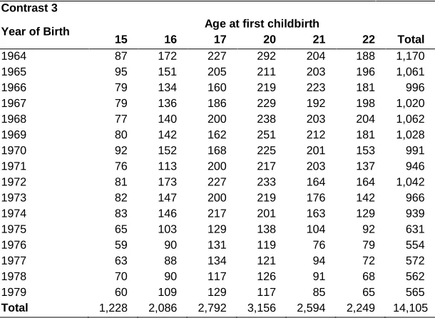
Table 1: Distribution of females in pseudo panel by cohort and age at first childbirth
Contrast 1
Year of Birth Age at first childbirth
18 19 20 21 Total
1964 226 258 292 204 980
1965 241 234 211 203 889
1966 258 224 219 223 924
1967 209 221 229 192 851
1968 249 225 238 203 915
1969 223 263 251 212 949
1970 213 234 225 201 873
1971 222 200 217 203 842
1972 248 227 233 164 872
1973 219 198 219 176 812
1974 246 200 201 163 810
1975 151 167 138 104 560
1976 127 125 119 76 447
1977 142 105 121 94 462
1978 140 118 126 91 475
1979 138 112 117 85 452
Total 3,252 3,111 3,156 2,594 12,113
Contrast 2
Year of Birth Age at first childbirth
15 16 17 18 19 Total
1964 87 172 227 226 258 970
1965 95 151 205 241 234 926
1966 79 134 160 258 224 855
1967 79 136 186 209 221 831
1968 77 140 200 249 225 891
1969 80 142 162 223 263 870
1970 92 152 168 213 234 859
1971 76 113 200 222 200 811
1972 81 173 227 248 227 956
1973 82 147 200 219 198 846
1974 83 146 217 246 200 892
1975 65 103 129 151 167 615
1976 59 90 131 127 125 532
1977 63 88 134 142 105 532
1978 70 90 117 140 118 535
1979 60 109 129 138 112 548
Table 1: (Continued)
Contrast 3
Year of Birth Age at first childbirth
15 16 17 20 21 22 Total
1964 87 172 227 292 204 188 1,170 1965 95 151 205 211 203 196 1,061
1966 79 134 160 219 223 181 996
1967 79 136 186 229 192 198 1,020 1968 77 140 200 238 203 204 1,062 1969 80 142 162 251 212 181 1,028
1970 92 152 168 225 201 153 991
1971 76 113 200 217 203 137 946
1972 81 173 227 233 164 164 1,042
1973 82 147 200 219 176 142 966
1974 83 146 217 201 163 129 939
1975 65 103 129 138 104 92 631
1976 59 90 131 119 76 79 554
1977 63 88 134 121 94 72 572
1978 70 90 117 126 91 68 562
1979 60 109 129 117 85 65 565
Total 1,228 2,086 2,792 3,156 2,594 2,249 14,105
Source: Own Calculations from DHS data
The choice of contrast groups is challenging, since the wrong control group can up-bias results. We choose these groups for two reasons: first, yearly differences are more important at early ages of life than later on, as most social characteristics are formed in the earlier years. For instance, the difference between a 16-year-old and a 17-year-old adolescent could directly translate into an extra year of education, while the difference between a 32-year-old and a 33-year-old woman does not necessarily imply a difference in educational attainment in either direction. Second, all human capital is under formation during adolescence and contrasting them with women over the age of 27 would result in an unfair comparison.
The following equation captures the reduced-form model:
(1)
for c=1, 2, …, C and t=1, 2, …, T, where
y
ct is the average of yit over all individuals, i,being i=1,2,….n; who belong to birth cohort c, at year t. Every year the average may change as it is built from different individuals and the total number of individuals, n,
ct ct ct
ct
ct
a
x
varies too. The dependent variable,
y
ct, will capture one by one the outcomes under study: quality of job, measured as informality; marriage market outcomes, measured as instability; partner’s job class; and being a victim of severe domestic violence. For children’s health outcomes we measure child mortality as defined by number per woman of children born alive who died, a rate that is also averaged across all women in each birth cohort. The termθ
a
ct indicates that a woman had her first child while in adolescence. To control for other individual characteristics, averaged by cohort, a vector x is included and an estimation will capture the results by estimators β. The disturbance term,ε
ct, includes a time-invariant individual effect,µ
c , which characterizes the pseudo panel data:(2)
For the standard linear estimation this error term is treated as an individual fixed effect, which with large numbers of observations tends to be eliminated, leaving only the random component of the equation (2). This linear estimation can be modified to a Random Effects Model (RE) by assuming that the time-invariant component of the error term,
µ
c, is identically and independently distributed, with zero mean (Baltagi 1995), which allows for inference for any representative sample. The existence of a random effect can and must be statistically tested before running the model.Estimators from pseudo panels are consistent if the original samples are large enough, and if each cell has sufficient observations, as is the case with our sample (see Table 1). Similarly, Instrumental Variable (IV) estimation statistical properties hold and are therefore feasible (see Mora 2006). Standard regression analyses are linear estimations for all continuous dependent variables. However, for those cases where endogeneity is an issue we use an Instrumental Variable (IV) as an additional regressor, presented in the following equation. The IV is chosen so it holds the property of not directly affecting the outcome with minimum correlation to unobservable characteristics (ε):
(3)
For each estimation we run the following standard algorithm to determine the best fit. First, we estimate a random effects model and test for the presence of the random effect using a Breush-Pagan test and retain the appropriate model, which could be either
ct c
ct
µ
υ
ε
=
+
ct ct ct
ct ct
ct
a
x
IV
a pooled data model – as this is more efficient in the absence of a random effect – or a random effects model. Second, we test for endogeneity of the wealth index using the first difference of this index as an instrument and running standard weak instruments and endogeneity tests based on the Durbin-Wu-Hausman statistic. If we fail to reject the exogeneity of the wealth index, a two-step least squares estimator is implemented using the previously described instrument; when the opposite is true, we use the preferred model of the previous step. For each preferred specification, first order autocorrelation tests are carried out by regressing residuals against their first lag. Finally, robust standard error estimators are implemented for each of our preferred models.7
Equations (1) and (2) include a ‘constant’ term,
α
ct, which is definitely non-constant as it varies over time and could be correlated with independent variables. Deaton (1985) has shown that whenever there are large numbers in the original sample the best estimation for this constant term is an approximation of its mean value. This value can be approximated by including a series of dummies per cohort in all cohorts included in the pseudo panel. A series of dummies is then included in all pooled data estimations, allowing for consistent and unbiased estimators as well as presenting a control for each cohort’s fixed effects.Job quality, measured as formality of the current job, is the first women’s outcome we consider. More formal jobs – technical, managerial, clerical, sales, and skilled manual workers – are considered to be of high quality, and informal jobs – independent workers with low educational levels, unremunerated family workers, domestic workers, unskilled manual workers, and agricultural jobs – are classified as being of lower quality.8 As explained above, we expect adolescent mothers to have lower-quality jobs, as they bear extra pressure for sustaining their children and therefore might accept any type of work.
Other outcomes relate to the marriage market. Stability is important for the well-being both of the children and of the women themselves, so we measure it by the number of partners a woman has had. Even if a woman is living in a stable relationship, her partner’s socioeconomic characteristics may differ by the woman’s age of childbearing (adolescent mothers versus those becoming mothers at age 20 or older). We also measure current partner’s job quality, using the same definition as for women’s job quality. In addition, we examine whether a woman has ever been physically abused
7 Women’s job quality showed first order autocorrelation for C3, multiple marriages for C2 and C3, severe
violence for C1, and child mortality for C1. The statistical significance of these estimates was unbiased.
8 Women occupied in the category of “services” were classified as holding formal jobs if they worked outside
by her current partner, and has therefore had her safety put at risk.9 Physical abuse, called severe domestic violence, includes attempted strangling or burning or threats or attacks by current partner using a weapon. Not having the full history of domestic violence for previous partners is another limitation of our analysis, but the information at hand proves a useful measure for this paper.
Finally, we measure children’s health by the proportion of children dead, derived from total live births per woman. We expect younger mothers to suffer higher mortality shares than women who postpone maternity, due to lack of knowledge of the many needs of children, as well as limited access to and use of the health care system. While having full information on each and every child’s exact dates of birth and death would be ideal, those data are unfortunately only available for babies born within the five years previous to the survey’s date, limiting the number of observations to small numbers that would not allow the application of our proposed statistical methodology.
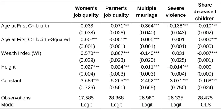
In a first attempt to account for full variability, in just one model we run standard logit estimations for the outcomes of interest − with the exception of share of deceased children, which follows an Ordinary Least Squares (OLS) estimation − using the pooled data for all cohorts under study and for women at least 30 years old by the time of the survey. Table 2 shows the results for all proposed outcomes, accounting for observable characteristics as well as age and age-squared as independent variables. For all outcomes except for partner’s job quality, age-squared is consistently positive and statistically significant, implying that age has a strong effect and supporting the construction of contrast groups that allow the estimation of a more refined effect. This also enables us to separate the impact of adolescent fertility for the youngest and oldest adolescents, as several critical socioeconomic and psychological characteristics differentiate them both intrinsically.
Although this research strategy reduces biases imposed by unobservable characteristics, both individual and familial, it is not infallible. There are complexities that prohibit the isolation of a pure effect of adolescent fertility that could still be confounded by particular familial and environmental characteristics of the studied outcomes, as happens with almost all other methodologies used to probe this question in the literature (e.g., Lee 2010). Moreover, this methodology is not able to account for women’s full retrospective information, as would be possible in a real panel. Perhaps the most significant drawback is the inability to account for adolescent mothers’ paternal household characteristics. To overcome this issue we have proxied such information using height; the following sub-section provides a detailed explanation of this choice.
9 Categorizing formal and informal jobs for women’s partners differed only in the sense that men working in
Table 2: Logit and OLS estimations for outcomes of interest. Pooled data − Colombia
Women's
job quality
Partner's job quality
Multiple marriage
Severe violence
Share deceased
children
Age at First Childbirth -0.033 0.071*** -0.364*** -0.138*** -0.010*** (0.038) (0.026) (0.040) (0.043) (0.002) Age at First Childbirth-Squared 0.002** -0.001** 0.005*** 0.001 0.000***
(0.001) (0.001) (0.001) (0.001) (0.000) Wealth Index (WI) 0.570*** 0.867*** -0.140*** 0.031 -0.007***
(0.029) (0.023) (0.020) (0.025) (0.001) Height 0.027*** 0.024*** 0.011*** -0.014*** -0.000
(0.004) (0.003) (0.003) (0.004) (0.000) Constant -3.689*** -5.265*** 2.452*** 3.071*** 0.168***
(0.726) (0.561) (0.665) (0.750) (0.024)
Observations 17,585 28,368 26,980 26,325 28,475
Model Logit Logit Logit Logit OLS
Source: Own Calculations from DHS data
*** p<0.01, ** p<0.05, * p<0.1. Robust Standard Errors in parentheses
3.1 Pre-existent socioeconomic conditions
One limitation of not having longitudinal data is the lack of retrospective information for all variables of interest, such as socio-economic conditions in the paternal household. Indeed, the only potentially relevant questions in the survey are: 1) if women recall their mothers being physically abused by their fathers, and 2) women’s mothers’ educational attainment. Neither of these questions would be suitable for this paper, as the former is not part of the 1995 DHS survey and implies a 25% loss of the sample, and the latter suffers from very low response rates (15%). Besides, domestic violence in the paternal house does not necessarily correlate with poverty (Ribero and Sánchez 2004). Similarly, maternal education could have changed between the time a woman lived in her father’s house and the date of the survey, and only 15% of women responded this question. Finally, as we are using information of respondents who are 30 years old or more, both questions may also suffer from memory recall issues, which could aggravate self-selection bias and create imperfect estimators.10
10 Mother’s educational attainment reaches only a 15% response rate, and therefore accounting for this
As presented in the previous section, adolescent motherhood is most common in socioeconomically challenged households in all countries where this unusual increase in adolescent fertility has presented, including the Colombian case. In an attempt to control for socioeconomic status of the paternal household of women in our study, we include a measure of women’s height as a proxy, assessed at the moment of the survey. This anthropometric measurement does not change over time, since women of all heights do not grow more than two centimeters after age 15 (see WHO’s universal growth charts for girls’ height11), so we can assume that a woman’s height at the time of the survey is almost identical to her height at the ages under study, 15 to 22 years.
Height is our proxy variable for pre-existing socioeconomic conditions from the paternal household, as there is sufficient evidence linking development and socioeconomic well-being with height, both at the aggregate and micro-data level. In the medical field, quality intake of nutrients has been quoted as the main determinant of fetus and early childhood development, related to birth weight and with long-term effects on adult health. These effects are empirically measured by mortality, height, weight, and brain development of children and adolescents (Adair et al. 2013; Bhutta 2013; Brozek et al. 1977; Kulin et al. 1982; Morgane et al. 1993). As expected, poor households can barely provide the necessary nutrition for pregnant women or young children to fully develop, which translates into lower heights at all ages. Child malnutrition effects are permanent. Even young children who improve nutritional conditions later in life fail to catch up at older ages (Malcolm 1970; Habicht et al. 1974; Coly et al. 2006; Victora et al. 2008).
From the economic and demographic point of view, the link between child malnutrition and adult height has been studied since Fogel et al.’s (1982) seminal paper connecting labor productivity and height in historical populations. Similar results have been found by authors using other dependent variables such as per capita income or socioeconomic strata (Steckel 1983; Kolmos 1990), and by others exploring data on subjects other than European males (Schultz 2002; Sunder and Woitek 2005; Strauss and Thomas 2007). Analysis of recent micro-data from DHS in developing countries (Subramanian et al. 2011) has also produced similar results, as has work with other micro-data information for Sri Lanka and India (Ranasinghe et al. 2011; Perkins et al. 2011) and analysis of 20th century data (Hatton and Bray 2010; Whincup et al. 2011; Hatton 2013).
These results are also supported by micro-data-level studies highlighting the role that malnutrition plays in lowering heights for individuals, when suffered either in utero or during the first years of life (Adair et al. 2013; Bhutta 2013; Brozek et al. 1977;
signs and statistical significance tend to replicate the results presented here, but the coefficients are larger in absolute terms.
Kulin et al. 1982; Morgane et al. 1993; Fogel 1994). Moreover, such effects are permanent, and cannot be counteracted even if children improve their nutritional intake later in life (Malcolm 1970; Habicht et al. 1974; Coly et al. 2006; Victora et al. 2008). Therefore, malnutrition and lower heights are more common in low-income households that fail to provide a good nutritional intake from rich and balanced diets (Behrman and Hoddinot 2001; Alderman et al. 2006), and height has proven to be a good proxy for socio-economic status in micro-data (Meisel and Vega 2006; Fogel 2000; 1997). This direct relationship between height and income has also been observed in Colombia (Meisel 2004; Ribero 2000).
We have double-checked this finding using specialized nationally representative micro-level data on health. Figure 2 shows this positive relationship between women’s height and educational attainment by age group, for each and every age group of women ages 18 to 49, using data from the 2007 National Health Survey, a nationally representative survey carried out by the Ministry of Health. When women’s heights are contrasted with their education levels (income level was not assessed), this direct correlation is clear.
Figure 2: Relationship between women’s height and socioeconomic status in Colombia, from National Health Survey (NHS), 2007
Source: Own Calculations from NHS-2007 data
Finally, there is evidence that correlates shorter height of girls to earlier onset of menarche in developed countries (Onland-Moret et al. 2005; Yousefi et al. 2013),
153
154
155
156
157
158
He
ig
h
t
Incompl. Primary Compl. Primary Compl. Secondary Compl. Tertiary
Schooling Level
18-29 30-39 40-49
which in turn may lead to longer exposure to adolescent fertility risk. However, this is not a major concern, as we limit our analysis to adolescents who became mothers at ages 15 or older. This earlier onset typically relates to access to better nutrition due to developmental advances that could even lead to obesity. However, Colombian women in this analysis include cohorts born in years when low nutritional intake was the biggest concern for children. Indeed, even if we look at the youngest cohorts in Colombia (girls born since 1993 from the 2010 DHS), as Figure 3 shows, there is no relationship between height and age at menarche in Colombia, with a correlation of just 0.072. Therefore, in this case we are not overly worried about height being strongly correlated with longer exposure to sexual activity.
Figure 3: Relationship between women’s height and age at menarche in
Colombia, 2010
Source: Own Calculations from DHS data
3.2 The data
The Colombian DHS has been designed to capture information on health programs, contraceptive use, fertility, infant and maternal mortality, and nutritional status. The DHS survey targets households, collecting information about women in their reproductive ages (12 to 50 in Colombia) and their children born in the previous five years. It also collects several anthropometric measurements – vaccination coverage and
50
10
0
15
0
20
0
He
ig
ht
in Cm
s
.
5 10 15 20
nutritional status of both mothers and their children – all of which are very relevant for this study. Colombia has run five DHS since 1990. This allows us to construct a pseudo panel and to satisfy the required statistical conditions (Deaton 1985), as the samples for each survey are sufficiently large.12
One concern may be a non-response bias for adolescent mothers, who may prefer not to answer this kind of survey. However, we are focusing on cohorts of adolescent first-time mothers aged 15–19, who had their first child between 1979 and 1994 and have been surveyed since 1995. The timing provides a lag between pregnancy and survey administration that should be long enough for women not to feel embarrassed about this issue. Also, there is no social stigma in Colombia about adolescent motherhood, and, because fertility reduction happened so fast, for older cohorts (those born before 1950) it was customary for women to marry at very young ages and to immediately have children (until 1985 the legal age for marriage without parental consent was 14 for girls and 16 for boys), while for more recent cohorts it is not an embarrassment but rather a way to stand out socially (Flórez Nieto et al. 2004). Finally, Table 3 presents evidence from vital records that the average proportion of adolescents becoming mothers for the 1998-2012 period was 21.84%, a rate very similar to DHS sample proportions of around 20.84%.
Table 3: Proportion of births to mothers aged 15 to 19 in total births in Colombia, from vital statistics and DHS data
Data from Vital Statistics DHS data
Year* Total Births (1) Births to Mothers
aged 15–19 (2)
%: 15–19/Total
(2)/(1) %: 15–19/Total
2000 752,834 160,226 21.28% 19.67%
2005 719,968 154,569 21.47% 22.22%
2010 654,627 147,307 22.50% 20.62%
*1995 is excluded, since birth records were not registered by the Vital Statistic Records at DANE that year. By then they were recorded by Registraduría Nacional del Estado Civil, with under-registration levels over 40%.
Source: Own Calculations from DHS data
12 All measurements capture the cohort’s mean measures instead of individual means. Thus, it can be assumed
3.3 Treatment and control groups
We run the exercise for two contrast groups at a time, for all econometric models proposed in Equation (1). Contrast one (C1) exploits natural discontinuity around age 20, comparing the outcomes of interest for older teenage mothers (18 to 19 years) and their children to those who became mothers between 20 and 21. Contrast two (C2) presents the differences between the youngest adolescents (15–17 years) and the slightly older ones (18–19 years). Contrast three (C3) presents the differences between the youngest and the oldest mothers with the same age difference: 15 to 17 years versus 20 to 22 years. The purpose of the three different contrasts is to have the best control group for each treatment, in an attempt to homogenize both socioeconomic and fertility characteristics.
The pseudo panel sums to a total of 12,369 observations for C1, 12,768 observations for C2, and 14,429 for C3. Cells are built from birth cohorts of women born between 1964 and 1979 who are at least 30 years old at the time of the survey, and uses age at first childbirth. All of the following econometric exercises include estimations of fixed effects by cohort, with inclusion of dummy variables for each cohort’s year of birth (following Deaton 1985), which is a valid estimator for the fixed parameter in all exercises estimating Equation (1) or (3). Including such dummies helps to reduce the bias of individual selection, transforming it into cohort selection bias, and all estimations are proven to meet the statistical needs of traditional models.
4. Results
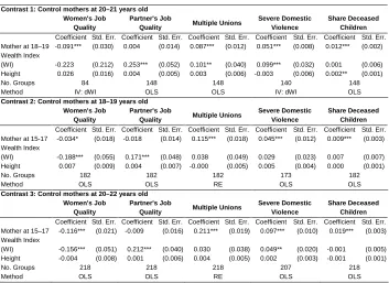
Our results are shown in Table 4, with its three panels corresponding to each contrast described above and appearing in the following order: C1, C2, and C3. Estimations with endogeneity issues include the relevant IV, when necessary. The selected IV is the household wealth index’s first difference, as poverty holds some memory (Blundell and Bond 2000).
Partners’ job quality shows the opposite results. As depicted in the second column, no contrast estimators are significant. That is, women 30 years or older who were adolescent mothers do not necessarily have higher probability of having a partner with low job quality for any contrast.
Table 4: Estimated results, contrast groups
Contrast 1: Control mothers at 20–21 years old
Women's Job Quality
Partner's Job
Quality Multiple Unions
Severe Domestic Violence
Share Deceased Children
Coefficient Std. Err. Coefficient Std. Err. Coefficient Std. Err. Coefficient Std. Err. Coefficient Std. Err. Mother at 18–19 -0.091*** (0.030) 0.004 (0.014) 0.087*** (0.012) 0.051*** (0.008) 0.012*** (0.002) Wealth Index
(WI) -0.223 (0.212) 0.253*** (0.052) 0.101** (0.040) 0.099*** (0.032) 0.001 (0.006) Height 0.026 (0.016) 0.004 (0.005) 0.003 (0.006) -0.003 (0.006) 0.002** (0.001) No. Groups 84 148 148 140 148 Method IV: dWI OLS OLS IV: dWI OLS
Contrast 2: Control mothers at 18–19 years old
Women's Job Quality
Partner's Job
Quality Multiple Unions
Severe Domestic Violence
Share Deceased Children
Coefficient Std. Err. Coefficient Std. Err. Coefficient Std. Err. Coefficient Std. Err. Coefficient Std. Err. Mother at 15-17 -0.034* (0.018) -0.018 (0.014) 0.115*** (0.018) 0.045*** (0.012) 0.009*** (0.003) Wealth Index
(WI) -0.188*** (0.055) 0.171*** (0.048) 0.038 (0.049) 0.029 (0.023) 0.007 (0.007) Height 0.007 (0.009) 0.004 (0.007) -0.000 (0.005) 0.005 (0.004) 0.000 (0.001) No. Groups 182 182 182 173 182 Method OLS OLS RE OLS OLS
Contrast 3: Control mothers at 20–22 years old
Women's Job Quality
Partner's Job
Quality Multiple Unions
Severe Domestic Violence
Share Deceased Children
Coefficient Std. Err. Coefficient Std. Err. Coefficient Std. Err. Coefficient Std. Err. Coefficient Std. Err. Mother at 15–17 -0.116*** (0.021) -0.009 (0.016) 0.211*** (0.019) 0.097*** (0.010) 0.019*** (0.003) Wealth Index
(WI) -0.156*** (0.051) 0.212*** (0.040) 0.030 (0.038) 0.049** (0.020) -0.001 (0.005) Height -0.004 (0.008) 0.001 (0.006) 0.004 (0.005) 0.002 (0.003) -0.001 (0.001) No. Groups 218 218 218 207 218 Method OLS OLS RE OLS OLS
*p<0.05; ** p<0.01; *** p<0.001. Robust Standard Errors in parentheses
Source: Own Calculations from DHS data
Column 3 presents long-term effects in the marriage market. As stated before, there is no stigma attached to adolescent motherhood when it comes to the marriage market in Colombia: instead we choose to observe relationship instability, measured by whether a woman has more than one union (including both marriages and consensual unions) rather than the probability of being part of a union.13 For all contrasts the results are positive and statistically significant, meaning that all adolescent mothers have a
13 In Colombia most couples have preferred consensual unions to marriages since the mid-1990s. Consensual
higher probability of being in more unstable partnerships as opposed to their controls. The range of percentage differences are large and statistically significant: 0.087, 0.115, and 0.211 for C1, C2, and C3, respectively. Part of the explanation may be that becoming a mother at a young age increases the likelihood of a woman becoming involved in unstable relationships, as having a baby may pressure a young couple to stay together when they would not have chosen to do so in the absence of the baby. Or, in the case of the mother who never formed a union with the baby’s father, as time passes and she re-enters the marriage market, having a baby is probably not a desirable trait for most potential mates, and might cause the relationship to be brief.
Another variable that helps us to measure the effect of partners’ characteristics on adolescent mothers is the probability of being a victim of severe domestic violence at the hands of their partner. As was the case with the analysis of women’s job quality, the first contrast is better measured with an IV model, and again all contrasts are statistically significant. For C1 the chances of being a victim of severe domestic violence increases by 0.051 percentage points for girls who became mothers at the age of 18 or 19 as opposed to those who postponed first childbirth to the ages of 20 or 21. For C2 these chances increase by 0.045 percentage points for adolescents who became mothers at ages 15–17 compared to older teenagers who delayed motherhood to ages 18 or 19, and for C3 the result is a staggering 0.097-percentage increase for adolescents who became mothers at ages 15–17 as opposed to women who postponed motherhood to ages 20–22. Therefore, adolescent motherhood reveals a higher vulnerability to very intense domestic violence, along with all the social and personal consequences this implies for women and their children. This result has not previously been highlighted in the literature and clearly indicates that public health policies cannot focus solely on the physical health of adolescent mothers and their children but should also provide psychological help. Their becoming mothers at a very early age may impact their individual self-perception in a negative way, leading them into more vulnerable situations and to the very risky behavior of coupling with abusive partners.
attained by females, while providing sanitary services for homes, including clean piped water, sewerage, and access to toilets. (See medical literature review in Miller and Urdinola 2010.)
These last two results – share of deceased children and domestic violence victimization – reveal the damaging impact on human capital for both these mothers and their children, along with a perpetuation of the poverty cycle in Colombia, a cycle in desperate need of being broken.
4.1 Internal Validity Test
In order to address possible confounding issues, we have run the same regression analysis for women born in the same cohorts, also restricted to those of at least 30 years of age at the time of the survey, but who became mothers at older ages, beginning at age 25. Under our proposed methodology, the main concern would be that we might confound differences in the outcomes due to adolescent motherhood and differences in just postponing motherhood at any age. Table 5 shows evidence suggesting that this issue is of no serious concern. For instance, women who became mothers at 25 or 26 years are contrasted with women who became mothers at ages 27 or 28 (top panel), as are first-time mothers at ages 25–27 with those who had their first babies at ages 28–30 (bottom panel). The results show no significant effects in any of these cases, and reassure that the impacts can be attributed to adolescent motherhood.
Table 5: Internal validity test
Validity Test A: Control Mothers at 25–26 years Women's Job
Quality
Partner's Job
Quality Multiple Unions
Severe Domestic Violence
Share Deceased Children
Coefficient Std.Err. Coefficient Std.Err. Coefficient Std.Err. Coefficient Std. Err. Coefficient Std. Err. Mother at 27–28 -0.018 (0.027) -0.008 (0.020) 0.015 (0.010) 0.016 (0.011) 0.003 (0.003) Wealth Index 0.419*** (0.121) 0.283*** (0.047) 0.005 (0.025) 0.006 (0.027) -0.002 (0.006) Height -0.010 (0.016) 0.004 (0.008) -0.006* (0.003) -0.004 (0.003) -0.001 (0.001) No. Groups 84 148 148 140 187 Method IV: dWI OLS OLS OLS OLS
Validity Test B: Control Mothers at 25–27 years Women's Job
Quality
Partner's Job
Quality Multiple Partners
Severe Domestic Violence
Share Deceased Children
Coefficient Std.Err. Coefficient Std.Err. Coefficient Std.Err. Coefficient Std. Err. Coefficient Std. Err. Mother at 28–30 -0.025 (0.018) 0.016 (0.019) 0.001 (0.010) 0.011 (0.009) 0.000 (0.004) Wealth Index 0.067 (0.064) 0.273*** (0.033) -0.019 (0.022) 0.009 (0.019) -0.009 (0.014) Height 0.010 (0.006) 0.009* (0.005) -0.002 (0.003) -0.001 (0.003) -0.001 (0.001) No. Groups 218 220 220 208 124 Method OLS OLS RE OLS IV: dWI
*p<0.05; ** p<0.01; *** p<0.001. Robust Standard Errors in parentheses
5. Conclusions
Our results show that women who gave birth during adolescence fared worse than women who postponed motherhood for only a couple of years in the following outcomes: women’s job quality, partner’s job quality, marriage market instability, severe domestic violence victimization, and share of deceased children.
We would like to highlight two important methodological issues. First, building a pseudo panel proves a reliable option for the study of long-term consequences of adolescent motherhood in developing countries that have access to more than one household survey with adequate data, such as the DHS, when longitudinal surveys are not available. Second, our intuition regarding the correct definition of both treatment and control group in each proposed contrast of this issue has been proven right. The parametric estimators show small differences when the treatment group is changed only slightly from older adolescent mothers (ages 18–19) to younger adolescent mothers (15–17 years). In order to have a clear perspective on this matter, we recommend that researchers and users of these statistics always be aware of the socio-economic and psychological differences between older and younger adolescents, as well as the implications of using slightly or much older women as control groups.
The main limitation of the use of a pseudo panel is its lack of longitudinal information that takes into account pre-existing conditions. For this reason, we use as a proxy women’s height to account for paternal household’s socioeconomic status. This variable may not be perfect, but it offers a good approximation of the issues at hand, as statistical exercises have shown that it performs well and helps to reduce biases introduced by unobservable individual characteristics.
challenge, therefore, is not to attract these young women into the educational system, but to retain them as they get older.
The diffusion of family planning services targeting these particular young women might help to improve school retention, but focusing on adolescents before the coming of age, around 18 in LAC, could become a social and legal battle. Instead, sexual education, mandatory in Argentina, Colombia, and Chile (among other LAC), could easily be reinforced and could reduce the probability of becoming a teen mother, as suggested by evidence from different studies in LAC and North America (Rodríguez 2008; Levine and Painter 2003; Pantelides 2002; di Cesare and Rodríguez Vignoli 2006; Azevedo et al. 2012). Most studies argue that providing access to sexual education and modern contraceptive methods, either by parents or in school, reduces the probability of becoming pregnant (Flórez Nieto 2005; di Cesare and Rodríguez Vignoli 2006; Rodríguez 2008), while other studies highlight the lack of available information about sexuality and reproduction, as earlier ages at first sexual intercourse and family environment are the leading risk factors for early motherhood in Latin America (Pantelides 2002; Flórez Nieto et al. 2004), as well as in the United States (Levine and Painter 2003).
Sex education should include teaching what is required to raise a baby. This means offering practical lessons that expose adolescents to the great demands of newborns in terms of time, healthcare, and money. Revealing all or most of the costs involved in having and raising a baby may help prevent adolescents from engaging in risky behavior, since teenagers are less prone than adults to fully consider the long-run consequences (Rabin and O'Donoghue 2000). This kind of ‘exaggerated’ education could provide a minimum knowledge of raising a baby, and teach adolescents when to look for medical help during pregnancy and the first year of life in order to reduce infant mortality.
psychological support for these women. It may be that certain behaviors related to early motherhood status also influence decisions in the marriage market, leading these women to choose abusive partners.
6. Acknowledgments
References
Adair, L.S., Fall, C., Osmond, C., Stein, A., Martorell, R., Ramirez-Zea, M., Sachdev, H., Dahly, D., Bas, I., Norris, S., Micklesfield, L., Hallal, P., and Victora, C. (2013). Associations of linear growth and relative weight gain during early life with adult health and human capital in countries of low and middle income: findings from five birth cohort studies. The Lancet 382 (9891): 525-534.
doi:10.1016/S0140-6736(13)60103-8.
Alderman, H., Hoddinot, J., and Kinsey, B. (2006). Long term consequences of early childhood malnutrition. Oxford Economic Papers 58(3): 450–474. doi:10.1093/ oep/gpl008.
An, C.B., Haveman, R., and Wolfe, B. (1993). Teen out-of-wedlock births and welfare receipt: The role of childhood events and economic circumstances. Review of Economics and Statistics 75(2): 195–208. doi:10.2307/2109424.
Auchter, M., Galeano, H., Balbuena, M., Zacarías, M., and Huespe, S. (2005). Riesgo al nacer en el hijo de madre adolescente. Corrientes. Argentina: Facultad de Medicina. Cátedras Enfermería Maternoinfantil y Pediatría II
Azevedo, J.P., Favara, M., Haddock, S.E., Lopez-Calva, L.F., Müller, M., and Perova, E. (2012). Embarazo adolescente resumen 2013. Washington, DC: World Bank Group. URL: http://documents.worldbank.org/curated/en/2013/01/18612719/ teenage-pregnancy-opportunities-latin-america-caribbean-early-child-bearing-poverty-economic-achievement-vol-1-2-embarazo-adolescente-resumen-2013
Baltagi, B. (1995). Econometric analysis of panel data. New York: John Wiley & Sons. Barrera, F. and Higuera, L. (2003). Embarazo y Fecundidad Adolescente. Análisis de
Encuesta de Coyuntura Social. (Working papers series No.24)
Behrman, J.R. and Hoddinott, J. (2001). An Evaluation of the Impact of PROGRESA on Preschool Child Height. Washington, D.C.: International Food Policy Research Institute (IFPRI). (FCND discussion paper104)
Berquo, E. and Cavenaghi, S. (2005). Increasing Adolescent and Youth Fertility in Brazil: A New Trend or a One-Time Event?. Paper presented at the Annual Meeting of the Population Association of America. Philadelphia, Pennsylvania: March 30 to April 2.
Blundell, R. and Bond, S. (2000). GMM Estimation with Persistent Panel Data: An Application to Production Functions. Econometric Reviews 19(3): 321–340.
doi:10.1080/07474930008800475.
Brozek, J., Coursin, D.B., and Read M.S. (1977). Longitudinal studies on the effects of malnutrition, nutritional supplementation, and behavioral stimulation. Bulletin of the Pan American Health Organization. 11(3): 237–249.
Burgos, L. and Carreño, S. (1997). Comparación de los factores de riesgo en dos poblaciones de embarazadas adolescentes nulíparas Revista Hospital materno-infantil Ramón Sorda. XVI(3): 104–111.
Buvinic, M. (1998). Costs of Adolescent Childbearing: A Review of Evidence from Chile, Barbados, Guatemala and Mexico. Studies in Family Planning. 29(2): 201–209. doi:10.2307/172159.
Coly, A.N., Milet, J., Diallo, A., Ndiaye, T., Bénéfice, E., Simondon, F., Wade, S., and Simondon, K.B. (2006). Preschool Stunting, Adolescent Migration, Catch-Up Growth, and Adult Height in Young Senegalese Men and Women of Rural Origin. Journal of Nutrition 136(9): 2412–2420.
Deaton, A. (1985). Panel data from time series of cross-sections. Journal of Econometrics. 30(1-2): 109–126. doi:10.1016/0304-4076(85)90134-4.
di Cesare, M. and Rodríguez Vignoli, J. (2006). Análisis micro de los determinantes de la fecundidad adolescente en Brasil y Colombia. Papeles de Población 48:107-140.
Driscoll, A. (2014). Adult outcomes of teen mothers. Demographic Research. 30(44): 1277–1292. doi:10.4054/DemRes.2014.30.44.
Ermisch, J. and Pevalin; D. (2003). Does a ‘Teen-birth’ have Longer-term Impacts on the Mother? Evidence from the 1970 British Cohort Study. Institute for Social and Economic Research. (ISER Working Paper Series. 2003-28).
Fernández, L.S., Carro, E., Oses Ferrera, D., and Pérez Piñero, J. (2004). Caracterización del recién nacido en una muestra de gestantes adolescentes.
Revista Cubana de Obstetricia Ginecología 30(2):
Flórez Nieto, C.E. (2000). Las Transformaciones Sociodemográficas en Colombia Durante el Siglo XX. Bogotá, Colombia: Banco de la Republica.
Flórez Nieto, C.E. and Núñez, J. (2002). Teenage Childbearing in Latin American Countries. Washington, D.C.: Inter-American Development Bank. (Documento CEDE 2002-01).
Flórez Nieto., C.E .Vargas, E., Henao, J., González, C., Soto, V., and Kassem, D. (2004). Fecundidad Adolescente en Colombia: Incidencia, Tendencias y Determinantes. Un Enfoque de Historia de Vida. Washington, D.C.: Inter-American Development Bank. (Documento CEDE, 2004-31).
Fogel, R.W. (2000). The Extension of Life in Developed Countries and Its Implications for Social Policy in the Twenty-first Century. Population and Development Review. 26(Supplement: Population and Economic Change in East Asia): 291– 317.
Fogel, R.W. (1997). New Findings on Secular Trends in Nutrition and Mortality: Some Implications for Population Theory. In: Rosenzweig; M.R. and Stark, O. (eds.)
Handbook of Population and Family Economics. Amsterdam: Elsevier: 433–481
doi:10.1016/S1574-003X(97)80026-8.
Fogel, R.W. (1994). Economic Growth, Population Theory, and Physiology: The Bearing of Long-Term Processes on the Making of Economic Policy. American Economic Review 84(3): 369–395
Fogel, R.W, Engerman S.L., Floud, R., Steckel, R.H., Trussell, J., Wachter, K., Sokoloff, K., Villaflor, G., and Margo, R.A. (1982). Changes in American and British Stature since the Mid-Eighteenth Century: a Preliminary Report on the Usefulness of Data on Height for the Analysis of Secular Trends in Nutrition, Labor Productivity, and Labor Welfare. National Bureau of Economic Research. (NBER Working Paper #890)
Gaviria, A. (2000). Decisiones: sexo y embarazo entre las jóvenes colombianas.
Coyuntura Social 84: 83–95.
Geronimus, A. and Koreman, S. (1992). The Socioeconomic Consequences of Teen Childbearing Reconsidered. The Quarterly Journal of Economics. 107(4): 1187– 1214. doi:10.2307/2118385.
Geronimus, A, Korenman, S., and Hillemeir, M.M. (1994).Does young maternal age adversely affect child development? Evidence from cousin comparisons in the United States. Population and Development Review 20(3): 585–609.
Gerstenblüth, M., Ferre, Z., Rossi, M., and Triunfo, P. (2009). Impacto de la maternidad adolescente en los logros educativos. Documentos de Trabajo Impacto 5(9): 1– 19.
Habicht, J-P., Yarbrough, C., Martorell, R., Malina, R.M., and Klein, R. (1974). Height, and Weight Standards for Preschool Children: How Relevant are Ethnic Differences in Growth Potential?. The Lancet. 303(7858): 611–615 doi:10.2307/ 2137602.
Hatton, T.J. (2013). How have Europeans grown so tall? Oxford Economic Papers 66 (2):349-372: doi:10.1093/oep/gpt030.
Hatton, T.J. and Bray, B.E. (2010). Long run trends in the heights of European men, 19th–20th centuries. Economics & Human Biology8(3): 405–413. doi:10.1016/ j.ehb.2010.03.001.
Hofferth, S. and Hayes, C. (1987). Risking the Future. Washington, DC: National Academy Press
Hogan, D.P., Sun, R., and Cornwell, G.T. (2000). Sexual and Fertility Behaviors of American Females aged 15–19 years: 1985, 1990 and 1995. American Journal of Public Health 90(9): 1421–1425. doi:10.2105/AJPH.90.9.1421.
Hotz, V.J., McElroy, S., and Sanders, S.G. (2005). Teenage Childbearing and Its Life Cycle Consequences: Exploiting a Natural Experiment. Journal of Human Resources 40(3): 683–715.
Hotz, V.J, Mullins, C.H., and Sanders, S.G. (1997). Bounding Causal Effects Using Data from a Contaminated Natural Experiment: Analyzing the Effects of Teenage Childbearing. Review of Economic Studies. 64(4): 575–603.
doi:10.2307/2971732.
Klepinger, D., Lundberg, S., and Plotnick, R.D. (1999). How Does Adolescent Fertility Affect the Human Capital and Wages of Young Women? The Journal of Human Resources 34(3): 421–448. doi:10.2307/146375.
Klepinger, D., Lundberg, S., and Plotnick, R.D. (1995). Adolescent Fertility and the Educational Attainment of Young Women. Family Planning Perspectives 27(1): 23–28. doi:10.2307/2135973.
Kulin, H.E., Bwibo, N., Mutie, D., and Santner, S.J. (1982). The effect of chronic childhood malnutrition on pubertal growth and development. The American Journal of Clinical Nutrition 36(3): 527–536
Lee, D. (2010). The early socioeconomic effects of teenage childbearing: A propensity score matching approach. Demographic Research 23(25): 697–736.
doi:10.4054/DemRes.2010.23.25.
Levine, D.I. and Painter, G. (2003). The Schooling Costs of Teenage Out-Of-Wedlock Childbearing: Analysis with a within-School Propensity-Score-Matching Estimator. The Review of Economics and Statistics 85(4): 884–900. doi:10.1162/ 003465303772815790.
Malcolm, L.A. (1970). Growth and Development of the Bundi Child of the New Guinea Highlands. Human Biology 42(2): 293–328
Martin, J.A., Hamilton, B.E., Sutton, P.D., Ventura, S.J., Menacker, F., and Kirmeyer, S. (2006). Births: Final data for 2004. National Vital Statistics Reports 55(1): Meisel, A. and Vega, M. (2006). Los orígenes de la antropometría histórica y su estado
actual. Bogotá, Colombia: Banco de la República.
Meisel, A. (2004). A tropical success story: a century of improvements in the biological standard of living, Colombia 1910–2002. Bogotá, Colombia: Centro de Estudios Económicos Regionales (CEER).
Miller, G. (2010). Contraception as Development? New Evidence from Family Planning in Colombia. Economic Journal 120(545): 709–736. doi:10.1111/j. 1468-0297.2009.02306.x.
Miller, G. and Urdinola, B.P. (2010). Cyclicality, Mortality, and the Value of Time: The Case of Coffee Price Fluctuations and Child Survival in Colombia. Journal of Political Economy 118(1): 113–155. doi:10.1086/651673.
Mora, J.J. (2006). El efecto de los títulos, la segmentación y el funcionamiento del mercado de trabajo: un análisis cuantitativo [Doctoral Thesis]. Alcalá, Spain: Universidad de Alcalá de Henares.
Morgane, P.J., Austin-LaFrance, R., Bronzino, J., Tonkiss, J., Díaz-Cintra, S., Cintra, L., Kemper, T., and Galler, J.R. (1993). Prenatal malnutrition and development of the brain. Neuroscience & Biobehavioral Reviews 17(1): 91–128 doi:10.1016/ S0149-7634(05)80234-9.
Onland-Moret, N.C., Peeters, P.H.M, van Gils, C.H., Clavel-Chapelon, F., Key, T., Tjønneland, A., Trichopoulou, A., Kaaks, R., Manjer, J., Panico, S., Palli, D., Tehard, B., Stoikidou, M., Bueno-De-Mesquita, H.B., Boeing, H., Overvad, K., Lenner, P., Quirós, J.R., Chirlaque, M.D., Miller, A.B., Khaw, K.T., and Riboli, E. (2005). Age at Menarche in Relation to Adult Height. The EPIC Study.
American Journal of Epidemiology 162(7): 623–632. doi:10.1093/aje/kwi260. Pantelindes, E. (2004). Aspectos sociales del embarazo y la fecundidad adolescente en
América Latina. Notas de Población 78:7–33 .
Perdomo, R., Álvarez, C., and Mejía, G. (2005). Evaluación nutricional en un grupo de adolescentes embarazadas en Cartagena, Colombia. Revista colombiana de Obstetricia y Ginecología 56(4): 281–287.
Perkins, J.M., Khan, K.T., Smith, G.D., and Subramanian, S.V. (2011). Patterns and trends of adult height in India in 2005–2006. Economics & Human Biology 9(2): 184–193. doi:10.1016/j.ehb.2010.10.001.
Rabin, M. and O'Donoghue, T. (2000). Risky Behavior Among Youths: Some Issues from Behavioral Economics. In: Gruber, J. (ed:). Risky Behavior among Youths: An Economic Analysis. Chicago: University of Chicago Press and NBER. Ranasinghe, P., Jayawardana, M.N.A., Constantine, G.R., Sheriff, M.R., Matthews,
D.R., and Katulanda, P. (2011). Patterns and correlates of adult height in Sri Lanka. Economics & human biology 9(1): 23–29. doi:10.1016/j.ehb.2010.09. 005.
Ribar, D. (1994). Teenage Fertility and High School Completion. The Review of Economics and Statistic 76(3): 413–424. doi:10.2307/2109967.
Ribero, R. (2000). Salud y productividad laboral en Colombia. Revista Desarrollo y Sociedad 45: 1–30.
Ribero, R. and Sánchez, F. (2004). Determinantes, efectos y costos de la violencia intrafamiliar en Colombia: Universidad de los Andes-CEDE. (Documento CEDE #002331).
Rodríguez, J. (2008). Reproducción en la Adolescencia en América Latina y el Caribe:
¿Una Anomalía a Escala Mundial?. Paper presented at Congreso de la
Asociación Latinoamericana de Población-2008. Córdova, Argentina.
Schultz, T.P. (2002). Wage gains associated with height as a form of health human capital. The American Economic Review 92(2): 349–353
Steckel, R.H. (1983). Height and per capita income. Historical Methods: A Journal of Quantitative and Interdisciplinary History 16(1): 1–7.
Strauss, J. and Thomas, D. (2007). Health over the life course. In: Schultz, T.P. and Strauss, J. (eds.). Handbook of development economics. Amsterdam: Elsevier: 3375–3474. doi:10.1016/S1573-4471(07)04054-5.
Subramanian, S.V., Özaltin, E., and Finlay, J.E. (2011). Height of nations: a socioeconomic analysis of cohort differences and patterns among women in 54 low-to middle-income countries. PLoS One 6(4): e18962. doi:10.1371/journal. pone.0018962.
Sunder, M. and Woitek, U. (2005). Boom, bust, and the human body: further evidence on the relationship between height and business cycles. Economics & Human Biology 3(3): 450–466. doi:10.1016/j.ehb.2005.03.003.
Upchurch, D.M. and McCarthy, J. (1990). The Timing of a First Birth and High School Completion. American Sociological Review 55(2): 224–234. doi:10.2307/ 2095628.
Victora, C.G., Adair, L., Fall, C., Hallal, P. Martorell, R., Richter, L., and Sachdev, H.S. (2008). Maternal and child undernutrition: consequences for adult health and human capital. The Lancet 371(9609): 340–357. doi:10.1016/S0140-6736(07)61692-4.
Whincup, P.H., Cook, D.G., and Shaper, A.G. (1988). Social class and height. British Medical Journal 297(6654): 980–981. doi:10.1136/bmj.297.6654.980-c.
WHO (2009). WHO Child Growth Standards: Methods and development. URL:
http://www.who.int/childgrowth/standards/velocity/technical_report/en/index.ht ml
Yousefi, M., Karmaus, W., Zhang, H., Roberts, G., Matthews, S., Clayton, B., and Arshad, S.H. (2013). Relationships between age of puberty onset and height at age 18 years in girls and boys. World Journal of Pediatrics 9(3): 230–238.