Patron: Her Majesty The Queen Rothamsted Research Harpenden, Herts, AL5 2JQ Telephone: +44 (0)1582 763133 Web: http://www.rothamsted.ac.uk/
Rothamsted Research is a Company Limited by Guarantee Registered Office: as above. Registered in England No. 2393175. Registered Charity No. 802038. VAT No. 197 4201 51. Founded in 1843 by John Bennet Lawes.
Rothamsted Repository Download
A - Papers appearing in refereed journals
Gower, J. C. and Payne, R. W. 1975. A comparison of different criteria for
selecting binary tests in diagnostic keys. Biometrika. 62 (3), pp. 665-672.
The publisher's version can be accessed at:
•
https://dx.doi.org/10.2307/2335526
The output can be accessed at:
https://repository.rothamsted.ac.uk/item/8v7v4
.
© Please contact [email protected] for copyright queries.
With 3 text-figures Printed in Great Britain
A comparison of different criteria for selecting
binary tests in diagnostic keys
B Y J. C. GOWER AND R. W. PAYNE
Rothamsted Experimental Station, Harpenden, Hertfordshire
SUMMARY
The problem of selecting tests to be used in nonprobabilistic binary diagnostic keys is discussed. Five selection criteria are compared and it is shown that all except a new criterion suffer from some deficiency. This criterion cannot be extended easily to cope with multi-response tests but another criterion, which behaves satisfactorily with binary tests, can be extended in some circumstances. The only criterion which can always be used with multi-response tests is least satisfactory for binary tests.
Some key words: Diagnostic keys; Error rates; Test selection.
1. INTRODUCTION
Consider n populations characterized by p binary characters. An individual sample from one of the populations may be assigned to its population of origin, or identified, by observing the values of its characters. In the following this process of observation will be termed testing and, unless otherwise stated, each test will be assumed to have two possible responses, termed positive and negative. A binary diagnostic key is a device for identifying samples, by applying the tests sequentially in a hierarchical manner. A sequence of test responses leading to an identification is termed a branch of the key. In general, branches will differ in length and the tests they use, although the same test can occur on several branches.
VOSB (1952) gives an interesting review of the historical development of keys.
To construct a key one requires a table giving the responses to thep tests for every popula-tion. There are four possible entries in this table: the response may be known to be positive for the whole population, or to be negative, or to be variable within the population, or the response may be unknown, there being no information available about the population value of the character concerned. Clearly, in the latter case, samples from the population may give either positive responses or negative responses and different samples need not give the same response. The first two types of response enable populations to be separated with certainty and when sufficient of these so-called fixed responses occur, all n populations can be identi-fied uniquely. Even when there are insufficient fixed responses to give complete separation of the populations, one may identify a sample to within a group of populations with certainty. Such groups may be further separated, either by using a probabilistic key (Good, 1970) or better by discriminant methods. In this paper we are concerned solely with certain identi-fication and therefore regard variable and unknown responses as equally uninformative, referring to both as unknown responses.
An optimum key may be denned as that with minimum average number of tests for identification. Alternative formulations include keys with minimum cost per identification or minimum number of different tests used (Gower & Barnett, 1971; Willcox & Lapage,
666 J. C. GOWEB AND R. W. PAYNE
1972). Except for dynamic programming algorithms, which effectively enumerate all possible keys (Garey, 1972), no exact algorithm is known for finding optimum keys. These are impracticable for most real data which may be concerned with several hundred populations and up to about one hundred characters (Bamett & Pankhurst, 1974). Several authors (Pankhurst, 1970; Hall, 1970; Morse, 1971; Payne, 1974) present algorithms giving approximate solutions. These all operate by selecting first the test that best divides all the populations into two sets. Various criteria, some of which are described below, have been used to define what is meant by the best test. After the first division, the chosen criterion is used to select the next test to be used with each subset of populations, and so on. Garey & Graham (1974) give examples showing that selecting tests in this way, without examining their later consequences, can lead to inefficient keys, but most authors claim that their algorithms work well in practice and certainly give keys as good as, if not better than, those prepared by intuitive methods.
This paper compares and contrasts three criteria used to determine the best test and also discusses two farther criteria, one of which is new. When all responses are fixed, these criteria all select the test that most nearly divides the populations into two equal groups. When some populations have unknown responses to a test, the populations concerned must be allocated to both groups. The criteria then differ but aim to select tests with few unknown responses while keeping the group sizes comparable.
We shall define pt to be the proportion of populations giving positive responses to
the ith test, qt to be the proportion of populations giving negative responses to the ith
test, and ri to be the proportion of populations giving unknown responses to the ith test.
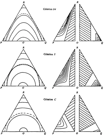
Thus, pi + q{ + rt = 1 and the ith test may be represented as a point Ti in barycentric
coordinates (Gower, 1967, p. 23). Thus in Fig. 1, the midpoint of PQ, labelled 0, represents the best possible test and R the worst possible test. Generally the better tests are those in the region of 0.
It may sometimes be preferable to identify some populations more readily than others, either because they occur frequently or because they are more important in some sense. In these circumstances one may ascribe a weight to each population and redefine pit qt and ri
as weighted proportions. In particular these weights might be prior probabilities for the populations.
2. T H E CRITERIA AND SOME PROPERTIES
We considered three criteria in detail: DV (Morse, 1971), S (Seshu, 1965; Gower & Barnett, 1971), and C (Gower & Bamett, 1971).
DV< = - 2ptqt - \rt{pt + qt), (1)
rt) log (pt + rt) + (qt + rt) log {qt + ri), (2)
(3)
To ensure that all three criteria are to be minimized, DV is here defined as the negative of the criterion proposed by Morse (1971). The left-hand side of Fig. 1 shows contours at equal intervals for each criterion. Tests lying on the same contour are regarded as equivalent. Gower & Barnett (1971) suggests that tests lying within a band around a contour might also be regarded as equivalent. When selecting one from several equivalent teste, additional considerations can be taken into account. For example, one can select the test with least
Selecting binary tests in diagnostic keys
667
cost, or the test that has been most used on other partially, orwholly, constructed branches of the key, or the test with fewest unknownresponses. The band is merely the region between contours with criterion values differing by a small constant, similar to the wider bands shown on the left-hand side of Fig. 1. The bandwidth is governed by the rate of change of the criterion.
The criterion DV has parabolic contours and C has circular contours. All three have roughly circular contours near 0. On the line PQ, where r = 0; DV = 2{p — £)8 — £ and
Criterion DV
Criterion 5
O
R
Criterion C
O
Fig. 1. Left-hand column: triangles show contours at equal intervals for each criterion. Right-hand column: triangles on the left, contours of type I error at intervals of 0-005; triangles, on the right, contours of type H error at intervals of 0-03. Shaded areas: regions with no error. Dotted line: contours tangential to PR and QR.
668 J. C. GOWEB AND R. W. PAYNE
C = 2(p — J)a differ only by a constant, and 8 behaves similarly to DV but its value initially increases less steeply from the minimum at 0. On the lines p — q = k, that is lines perpendicular to PQ, DV increases linearly with r and C = ^jfc2 + 3r2); 8 behaves similarly to C increasing less steeply from p = \.
Definite separation of populations cannot be guaranteed when either p or q is zero, and therefore such tests, termed indefinite below, should only be used when there are no alterna-tives. Yet the contours for all three criteria cut the lines Pi? and QR. The bigger the areas of the contours that touch the lines PR and QR the fewer indefinite tests will be selected in preference to tests giving definite separation. Tangential contours are shown as dotted lines in Fig. 1. When p = 0 the contour for C touches QR at q = 0-75, r = 0-25, the contour for DV at q = 0-5, r = 0-3 and the contour for S at q = 1 - 1/e = 0-6321, r = 1/e = 0-3679. It is clear that DV encloses the greatest area and that 8 encloses slightly more than C. This implies that DV is less susceptible to accepting indefinite tests than are 8 and C. The criteria could be modified to reject tests lying on the boundaries, but tests near the boundaries should also be excluded because they are inferior to tests near P and Q with greater criterion value; see the discussion of type I error below.
3. EBBOBS ASSOCIATED WITH THE OBTTEBIA
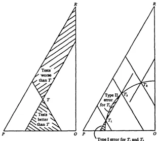
In some situations it is clear that one test is better or worse than another. If for two tests Ttand Ty
max {pt,qt) > m a x ( ^ , ^ ) , m i n ^ . f t ) > m i n i f y ) , (4)
then T< is certainly a better test than Tjt because more samples will be assigned definitely
to both the positive and the negative response groups. Conversely if
max (pt, qt) < max (pp q,), min (pit qt) < min (pp qt), (5)
then Ti is certainly a poorer test than Tj. Equations (4) and (5) are expressed in terms of
max (pit q{) and min (pt, qj because for any test, an equivalent test can be defined which
interchanges the definitions of positive and negative responses. In the following we assume that this relabelling has been done to make pi ^ qt and pj ^ q^. Thus we only consider the
region to the left of OR. Regions containing tests better and worse than a given test T are shown on the left-hand side of Fig. 2. Tests in the unshaded regions are not clearly better or worse than T.
Using any of the criteria to compare T with other tests, two types of error may arise. A type I error occurs when the criterion defines a test to be poorer than T, though (4) shows that it is better, hence it is possible for T to be selected in preference to other, better, tests. A type I I error occurs when the criterion defines a test to be better than T though (5) shows that it is worse. Thus, if there were no better tests available, the criterion might select a test worse than T in preference to T. No criterion with convex contours can have tests with type I I errors only, except on the boundary PQ or if they contain sections parallel to PR; see criterion BP, below. On the right-hand side of Fig. 2, tests Tj, T2 ^ d Tz are, respectively,
tests with both type I and type I I errors, type I error only, and no errors. For the criteria DV, 8 and C the areas associated with both errors have been calculated for a range of tests. As these errors are symmetric about 0.R, contours of equal error have been shown for both types in the pairs of triangles on the right-hand side of Fig. 1. The left-hand triangle gives the type I errors and the right-hand triangle the type I I errors. The contours are at the same
Selecting binary tests in diagnostic keys
669
intervals for the three criteria; for type I errors at step lengths of 0- 005 and for type II errors
at step lengths of 003, taking the area of PQR as ^3. The circle criterion C is least prone to
both types of error followed by DV, while S is poorest in both respects. Although DV and S
have zero type I and type II errors near 0, the most useful region, C has only negligible error
in this region.
O P
Type I error for 7i and Tt
Fig. 2. Left-hand triangle: regions containing tests definitely better and definitely worse than T. Right-hand triangle: test T1 has both type I and type II errors, test Tt type I error
only and test Ts no error.
Fig. 3. Left-hand triangle: contours of BP through p = J, q = J for k = 0, 1 and 2. Right-hand triangle: contours at equal intervals of GP with d = \.
670 J . C. G O W E B AND R. W . P A Y N E
Criteria with no type I or type I I errors can be defined. Barnett & Pankhurst (1974) use
where k = n, but we shall consider other nonnegative integer values of k. Figure 3 shows contours through the pointy = \, q = J for k = 0, 1 and 2. When k < 1 type I and II errors occur; when k = 1 a test T on Ax C has vestigial type II error on the line ArT. When k > 1
neither type I nor type I I errors occur. However, tests on any of the lines A^Bj (j = 0, 1,2) are considered equivalent, whereas tests on OR are clearly the best of such groups.
Contours which are isosceles triangles based on PQ avoid this deficiency and will have zero type I and type I I error, provided their base angles are less than 277/3. By increasing the base angle as the triangles increase in size, contours may be prevented from cutting the lines PR and QR, so avoiding indefinite tests. The following criterion fulfils all these con-ditions:
i,qi)}], (6)
where 0 < 6 < 1. As the triangular contours increase in size their slopes increase from to .^3 as shown on the right-hand side of Fig. 3. Choice of 6 governs how heavily one wishes to guard against using unknown responses. High values of 6 give contours which include more unknown responses than those for low values of 6. Values of 6 near zero will not dis-tinguish very well between tests on PQ, culminating in regarding all these as equivalent when 6 = 0. If 0 = 1 were allowed, (6) would become av{ = — min (pit q{), which gives nested
equilateral triangle contours, corresponding to (4) and (5), which have type II errors.
4. TESTS WITH MORE THAN TWO RESPONSES
It is always possible to recode a test with m responses as m — 1 binary pseudotests. This is often sufficient but may be unsatisfactory when, costs of tests are significant. For example, suppose the n populations can be separated by a single test with n responses. When this test is regarded as (n — 1) pseudoteste the criteria discussed above are unlikely to select just from the pseudotests and will therefore generally produce a more costly key. Thus methods are needed to assess multiresponse tests directly.
To compare a test with m^ responses to one with m2 > m^ responses we note that they both may be regarded as dividing the populations into mi classes, but that with the former m2 — w^ of the classes are empty. When all responses are fixed we can choose M = max (m{) and
amend S{ and C4 to become
m(
ST
= S
where p^ is the proportion of populations in the jth. class of the tth test. Thus both S? and Cf rank the tests independently of the choice of M. It might seem that BP extends similarly to give
1 M
BPf= £
1-1 Pa- M
However, even with M = 3 the two sets of tests responses (J, \, 0) and (J, f, 0) both give BP* = J which does not preserve the ranking for M = 2. Thus this method of extension is
Table 1. Performance of the five criteria
Criterion
671
Characteristic Computation Type I errors \ Type II errors/ Prevention of
in-definite tests Performance for
r constant Weighting of
un-known responses Multiresponse ex-tension • Provided ** Worsens DV Efficient Intermediate Good Perfect Fixed No
k > 1.
with increasing S Inefficient Largest errors Satisfactory Perfect Fixed Yes k. C Efficient Errors smaller
than DV or S Satisfactory Perfect Fixed
Only when all responses fixed BP Efficient None* Poor** Poor Control-lable*** Unsatisfactory GP Efficient None Perfect Perfect Controllable No
*** The choice of k = n (Barnett & Pankhurst, 1974) seems excessively restrictive.
unacceptable. Pankhurst (1970) has an alternative method of extension which biases against tests with more than two responses.
With unknown responses we define
i-i
and #* remains independent of M. However we have been unable to find any similar exten-sion for Cf or BP? . It might seem that a suitable extenexten-sion of Cf would be
M
With M = 3, this would regard the two-response test (plt p2, r) as equivalent to the
three-response test {p1,P2> 0, r) although the former separates the populations into groups with
sizes proportional to (j>i + r, pz + r,0) compared with (px+r, p% + r,r) for the latter. Thus
the three-response test is better because it offers the possibility of separation, should samples actually occur with the third level of response.
Neither DV nor GP seem to extend simply to include tests with more than two responses.
5. CONCLUSION
Criteria for selecting binary tests with unknown responses, have been shown to have the following possible deficiencies: (i) they may produce type II and/or type I errors; (ii) they may select indefinite tests in preference to definite tests; (iii) for constant r, they may regard tests for which p =(= q, to be as good as a test with p = q. Apart from such clear deficiencies, there is the more subjective question of deciding how much weight should be given to un-known responses. The possibility of extending a criterion to deal with multiresponse tests is important for some applications. Finally, as the calculation of selection criteria occurs in the innermost loops of computer programs for generating diagnostic keys, their
672 J. C. GOWEB AND R. W. PAYNE
tional efficiency is important. Table 1 sete out the performance of the criteria in these respects.
For tests with only two responses GP is best on all counts, but C and DV are satisfactory. In the multiresponse case, only S seems to be suitable unless all responses are fixed.
REFERENCES
BABNETT, J. A. & PANKHUBST, R. J. (1974). A New Key to the Yeasts. Amsterdam: North Holland.
GABBY, M. R. (1972). Optimal binary identification procedures. S.I.A.M. J. Appl. Math. 23, 173-86.
GABBY, M. R. and GRAHAM, R. L. (1974). Performance bounds on the splitting algorithm for binary testing. Ada Informatica 3, 347-65.
GOOD, I. J. (1970). Some statistical methods in machine intelligence research. Math. Biosci. 6, 186-208.
GOWEB, J. C. (1967). Multivariate analysis and multidimensional geometry. Statistician 17, 13-28. GOWEB, J. C. & BABNBTT, J. A. (1971). Selecting tests in diagnostic keys with unknown responses.
Nature 232, 491-3.
TTAT.T., A. V. (1970). A computer-based system for forming identincation keys. Taxon. 19, 12-8.
MOBSB, L. E. (1971). Specimen identification and key construction with time sharing computers.
Taxon 20, 269-82.
PANKHUBST, R. J. (1970). A computer program for generating diagnostic keys. Computer J. 13, 145-51.
PAYNE, R. W. (1974). Genkey: a program for constructing diagnostic keys. In Biological Identification
with Computers, Ed. R. J. Pankhurst, pp. 65-72. London: Academic Press.
SESKU, S. (1965). On an improved diagnosis program. I.EM. Trans. Electronic Computers. EC-14, 76-9.
Voss, E. G. (1952). The history of keys and phylogenetic trees in systematic biology. J. Sci. Labs.
Denison Univ. 43, 1-25.
WTLCOX, W. R. <fe LAPAGE, S. P. (1972). Automatic construction of diagnostic tables. Computer J. 15, 263-7:
[Received August 1974. Revised March 1975]