DEMOGRAPHIC RESEARCH
VOLUME 31, ARTICLE 6, PAGES 137–160
PUBLISHED 9 JULY 2014
http://www.demographic-research.org/Volumes/Vol31/6/ DOI: 10.4054/DemRes.2014.31.6
Research Article
Male fertility in Greece: Trends and differentials
by education level and employment status
Alexandra Tragaki
Christos Bagavos
© 2014 Alexandra Tragaki and Christos Bagavos.
This open-access work is published under the terms of the Creative Commons Attribution NonCommercial License 2.0 Germany, which permits use, reproduction & distribution in any medium for non-commercial purposes, provided the original author(s) and source are given credit.
1 Introduction 138
2 Data and methods 140
3 Results 142
3.1 The male side of fertility 142
3.2 Male fertility differentials by education level and employment
status 146
3.3 Decomposition of trends in male fertility 148
4 Conclusion 152
5 Acknowledgments 153
References 154
Appendix A 158
Appendix B − Construction of educational level variable 159
Male fertility in Greece: Trends and differentials
by education level and employment status
Alexandra Tragaki1
Christos Bagavos2
Abstract
BACKROUND
More than downplayed, the role of men in the demographic analysis of reproduction has been entirely neglected. However, male fertility can be an important issue for exploring how economic and employment uncertainties relate to fertility and family dynamics.
OBJECTIVE
This paper intends to study fertility variations over time, relying solely on data referring to father’s socio-demographic characteristics; in particular, their age, education level, and employment status.
METHODS
We use a combination of Labor Force Survey and Demographic Statistics data on population and Vital Statistics on births to estimate male fertility indicators and fertility differentials by education level and employment status, for the period 1992–2011 in Greece. In addition, over-time developments in male TFR are separated into structural (education-specific and employment-specific distributions) and behavioral (fertility, per se) changes.
RESULTS
We find that the male fertility level is declining, the fertility pattern is moving into higher ages, and the reproduction period for men is getting shorter. From 1992 up to 2008, changes in male fertility were mostly driven by behavioral rather than compositional factors. However, the decline of male fertility over the period of economic recession (2008–2011) is largely attributed to the continuous decrease in the proportions of employed men.
CONCLUSIONS
The study suggests that male fertility merits further exploration. In particular, years of economic downturn and countries where household living standards are mostly associated with male employment, a father’s employability is likely to emerge as an increasingly important factor of fertility outcomes.
1. Introduction
When it comes to fertility research, demographic analysis is conventionally female-oriented. Most theories developed to detect and explain changes in human fertility are not gender-specific, for they rarely, if ever, examine male and female behavior separately, as is the case in mortality and migration research. Fertility analysis focuses largely on mother’s socio-demographic characteristics, such as age, race, marital and employment status or level of education, in order to identify explanatory factors behind differing fertility rates and overtime variations. Significantly less attention has been given to men; a father’s income has for long been the only male feature involved in relevant analysis. Consequently, all fertility indicators are female-dominated: fertility rates, whether general, total or age-specific, relate living births to the age-sex group at risk. Therefore, all main fertility measures are in fact female fertility measures. More than downplayed, the role of men in the demographic analysis of reproduction has been entirely neglected.
Zhang 2011: 3–6). For countries with poor statistical records and high infant mortality, this is a serious weakness. Surveys conducted in developed countries are not spared such shortcomings, either. Unlikely though it may seem, discrepancy in numbers of children reported by male and female respondents is found to be larger for children spending less than six months per year with their father (Juby and Le Bourdais 1999).
During the recent decades, demographic interest in changing family attitudes and new fertility patterns have provided some good reasons why males should be involved in the investigation of fertility determinants. With marriages becoming less stable and anything but a prerequisite for childbearing, men and women do not necessarily share the same fertility experiences any more. When couples’ stability ceases to be the norm, variations in the intensity of fertility across gender may be more significant than mortality or nuptiality differentiations would justify. Increasing divergence in reproductive experiences between men and women revalidates the importance of men’s involvement in fertility research, and argues in favor of charting male fertility as meticulously as that of females.
Within the last couple of decades, scientists of different disciplines, such as biology, medicine, pharmacology, sociology, and demography have found interest in the male side of human reproduction. A slowly developing literature is currently being built on two unevenly growing pillars: one of a medical and one of a sociological orientation.
The main body of male fertility literature is made up of studies with a purely biological and medical interest, with the aim of investigating mechanisms responsible for male infertility and sterility. A variety of factors – physical, behavioral, and environmental – have been examined as plausible determinants of semen quality or as hormone disruptors capable of influencing the fertility of men. According to Poston and Chang (2005), studies of medical orientation count for no less than two-thirds of all studies on male fertility. Despite their numerical importance, those studies are out of the scope of this research and will not be further discussed in this paper.
In more developed countries, interest in male fertility is very recent, though the lack of relevant studies has been repeatedly mentioned (Brouard 1977; Forste 2002; Poston and Chang 2005). The most common approach compares male age-patterns with female ones, and evaluates gender differentiations across factors affecting fertility levels (Ravanera and Fernando 2003; Bianchi 1998). The main common finding suggests that male and female fertility differentials exist in almost all societies: age-specific fertility patters (Bachu 1996; Paget and Timæus 1994; Kiernan and Diamond 1983) and dynamics (Ventura et al. 2000; Coleman 2000) differ between men and women. A few more focused studies highlight some generally overlooked issues. Bronte-Tinkew et al. (2009) examine social factors associated with higher-order fertility among males; Guzzo and Hayford (2010) provide sufficient evidence for men and women being subject to different selection forces of unmarried first-time parenthood, as well as to divergent subsequent fertility behavior; Lappegård and Rønsen (2013) examine socioeconomic differences in multi-partner male fertility in Norway. Lately, male fertility has been incorporated in studies exploring the way economic and employment uncertainties relate to fertility and family dynamics in the developed world (Kreyenfeld et al. 2012; Sobotka et al. 2011).
This paper intends to study fertility variations over time, relying solely on data referring to father’s socio-demographic characteristics. Based on aggregated birth data annually supplied by the Hellenic Statistic Authority (EL.STAT.), this work aspires to clarify the patterns, levels and changes of male fertility in Greece during the last two decades; to our knowledge this aspect has not been addressed before. The most common measures of fertility used in demographic analysis will be recalculated on the basis of male population so as to provide the age pattern of male fertility. Additionally, we investigate fertility differentials by education level and employment status. Moreover, using a decomposition method, we examine the distributional effect of a father’s education level and employment status on fertility. Over-time developments in TFRM are therefore decomposed into structural (education-specific and employment-specific distributions) and behavioral (fertility alone) changes. Our analysis covers a twenty-year period, going from 1992 to 2011; within this time period notable fertility variations occurred against a rapidly changing social and economic environment.
2. Data and methods
fathers’ demographic and socio-economic attributes, such as age, education level and employment status as compiled for the National Vital Statistics, and provided at aggregate level on an annual basis by the Hellenic Statistical Authority (EL.STAT). Births supplied by EL.STAT. (2013) are tabulated by five-year age groups, by six different categories of employment status, and by five different educational groups3. The average male population by age, education level and employment status is deduced from two different sources: demographic statistics (Eurostat 2013a) and LFS (Eurostat 2013b; 2013c). The age, education and employment distribution, as issued by the annual results of the Labor Force Survey4, is applied to the average population provided by demographic statistics (for more details see Appendix). Male fertility indicators, i.e. the age-specific fertility rates and the total fertility rate (TFR), are therefore calculated using birth data tabulated by father’s age, education level, and employment status. The high quality of male fertility data offers a great advantage to this study, since the robustness of the results is not affected by simplistic assumptions, which are otherwise necessary.
Age-specific fertility rates, total fertility rate and mean age at fatherhood are estimated for every year over the period 1992‒2011 to describe trends in male fertility. The examined period is divided into three distinct sub-periods conditioned by fertility developments. Broken down by level of education and employment status, those measures highlight some noteworthy differences across distinct population subgroups, along with overtime variations.
Thereafter, we aim to explore fertility differentials in relation to two wide-range socio-economic developments the Greek population has gone through within the recent decades: the increasing educational attainment and varying employment rates of the male population. While the influence of shifting educational and occupational distributions of the female population on childbearing decisions has been visited (Rindfuss et al. 1996) and revisited (Kögel 2004; Engelhardt and Prskawetz 2004; Adserà 2004), the relevant effect of changing male distributions remains under-studied. A decomposition method is therefore applied to dissociate the impact of compositional effects (education differentials and employment status variations) from behavioral effects (fluctuations in fertility) on the above-mentioned variations of TFR.
As repeatedly mentioned by previous works (Joyner et al. 2012; Zhang 2011; Greene and Biddlecom 2000; Rendall, et al. 1999; Poston and Chang 2005), under-count is one major issue to deal with when focusing on male-related birth data. The number of births tabulated by father’s information falls behind the total number of
3 A detailed description of tabulated data provided by El.STAT, as well as the construction of the education
level and the employment status variables, for the purpose of this work, are explained in the Appendix.
4 For detailed information on technical issues concerning the Labor Force Surveys, please see Eurostat
births annually registered. In Greece, the percentage of birth data suffering from missing information about fathers goes from less than 3% in 1992 up to almost 7% in 2011. Far from being a simple coincidence, percentages rise in line with the non-marital birth ratios; yet neither all certificates of non-marital births lack information about father nor does all missing information refer to non-marital births. Not surprisingly, the risk of incomplete registrations is not equally distributed across the Greek population. In 2011, data about father’s age, education level and employment-status were under-reported for more than half of babies born to mothers less than 20 years old, and for one out of five babies born to mothers of low education level. A methodological assumption about missing data was therefore necessary. The procedure here decided upon was to exclude any incomplete birth registration from our analysis, rather than to proportionately distribute unknown births to various age or education groups. This opted choice might slightly underestimate the total fertility rate, while the alternative would inevitably bias fertility of various sub-groups, in that the risk of underreporting varies with parents’ demographic characteristics. In spite of this shortcoming, information about father’s demographic profile at time of birth is available for almost 95% of all births in Greece. This is considered sufficient to efficiently chart and adequately understand male fertility patterns and their variations. Measuring male fertility is expected to offer interesting as well as meaningful insights into the dynamics and determinants of human reproduction and family formation behavior.
3. Results
3.1 The male side of fertility
Male fertility is hereafter described by the two most widely used indicators, the male total fertility rate (TFRM) and the male age-specific fertility rates (ASFRM). These are the same indicators applied in female fertility research, slightly modified only in respect to the upper age-limit, which is pushed up to 64 years of age in order to capture the longer fertile period in a man’s life. Ten ASFRs (15‒19, 20‒24, … 55‒59 and 60‒64) are used in the calculation of TFRM. The very limited numbers of births to fathers below 15 or above 65 years of age are included in the first (15‒19) and the last (60‒64) age groups, respectively.
first one goes from 1992‒1999, when fertility follows an uninterrupted declining trend; the already low levels of TFRM further shrank down to 1.18 children per man by 1999. The second period covers the years 2000‒2008 when TFRM slowly rebounds to reach 1.28 children per man by 2008. The third period, started in 2009, is marked by a new (and more abrupt) fertility decline, as TFRM plummeted down to 1.15; this period coincides with the currently unfolding economic recession. Beneath the wavy surface of TFRM variations, interesting structural and compositional changes have been occurring. Those aggregate fluctuations reflect broad changes in male fertility patterns in respect to age, education and labor force participation.
Figure 1: Male total fertility rate and mean age at fatherhood, Greece, 1992‒2011
Note: Left axis refers to male TFR (in columns); right axis refers to the mean age at fatherhood (line).
Source: Own calculations based on EL.STAT.: National Vital Statistics, Eurostat: Demographic Statistics and Labor Force Surveys, 1992‒2011.
Despite the fact that it steadily peaks at the same age-class (30‒34 years), the shape of ASFRM curve has gone through some modifications during the years examined: the curve shifted slowly to the right, got shorter and slightly narrower (Figure 2). Each of those movements graphically illustrates a noteworthy fertility development. First, the male fertility pattern shows ageing, as the curve shifts to older ages; second, the level of total male fertility is declining, as the peak gets lower; and, third, the reproduction period is getting shorter, as the width of the curve narrows.
Figure 2: Age specific fertility rates for males, for selected years
Source: Own calculations based on EL.STAT.: National Vital Statistics, Eurostat: Demographic Statistics and Labor Force Surveys, 1992–2011.
increases. Only men falling in the middle age group (between 30 and 34 years of age) have they experienced smooth fertility changes.
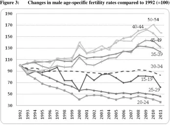
Important differences in age-specific rates, as well as changing relative impact of each age group on total rate, are masked under similar fertility levels. In both 1995 and 2009 total male fertility was estimated at 1.27 children per man. Within this fourteen-year interval, the age-specific fertility rates decreased for all ages below 30: the rate of change varied from -7% for the ages 15‒19 down to -33% for 25‒29. Age-specific fertility rates remained almost stable for men in their early 30s while all age groups above 35 years experienced remarkable increases: the rate of change reached 63% for 50‒54 followed by 57% for 40‒44. Shifts in the effect of each age group on total fertility rate are equally notable. In 1995 men below the age of 30 accounted for almost 31% of total fertility, compared with roughly 20% in 2009.
Figure 3: Changes in male age-specific fertility rates compared to 1992 (=100)
Note: The values plotted are the ratio of a given age-specific fertility rate in year t to the same rate in 1992. Changes here plotted have different effects on rates of overall change, subject to the fertility level of each age group.
It is also worth mentioning that in the last couple of years, all age groups register a clear and, in certain cases, steep decline in their fertility rates. The concomitant fall in fertility across ages explains the abrupt fall in total male fertility since 2009.
3.2 Male fertility differentials by education level and employment status
Educational groups are supposed to have different fertility experiences and follow separate trends. Research findings suggest persisting differences in fertility regarding mother’s education: higher fertility is confined to the less educated (Lewis and Ventura 1990; Yang and Morgan 2003; Bagavos 2010; Rendall et al. 2010). As the level of educational attainment rises, childbearing is postponed to later ages, and TFR declines. Though there is a general scientific consensus regarding education’s direct effect on women’s fertility, hardly anything is known about educational differentials of fertility across men.
Based on the highest education level attained, age-specific fertility rates have been calculated for three discrete education groups: Level 1 comprises men with the so-called “basic education” that requires 9 years of schooling; Level 2 comprises men who have completed the secondary education, in other words 12 years of schooling; and Level 3 comprises men that have received a university degree. Regarding employment status, two different groups are hereafter identified: employed and non-employed. The latter comprises all categories of inactive male population; namely, students, retirees, and the unemployed. Four years are displayed: 1992, 2000, 2008, and 2011 (Figures 4).
Our findings show that decreases in fertility rates have occurred disproportionately for the less educated men. During the 1990s, lower educational attainment is linked with a younger fertility pattern and higher fertility rates; the latter is under question since the turn of the millennium. From 2000 onwards, fertility curves for the highly educated men (Level 3) peak substantially higher than those for the least educated (Level 1) and are close enough to those with 12 year schooling. It needs to be mentioned that since fertility rates here estimated are period TFRs, their levels are subject to relative age-distribution across fertile years, as well as to population shares of each education group. As Level 1 registers the fastest diminishing population shares, its contribution to the calculation of total TFR lessens as time goes by; the opposite happens to the impact of Level 3.
off-set the drops during the years 1992‒2000 and 2008‒2011: Level 2 experienced the most important fall during the 90s while Level 3 was mostly affected during the last three years. The period 2008‒2011, the years of recession for the Greek economy, has a crucial effect on fertility dynamics. Within only three years, TFRM dropped 10% and reached the lowest low level of 1.15. Moreover, the childbearing pattern is moving further into higher ages, and this is not due to educational increases alone. Shifts towards older ages are common to all three education clusters, as shown in the way the mean age at fatherhood evolutes over time; such shifts are, however, stronger for better educated men — a trend that implies the strong association between education level and delayed childbearing.
Table 1: Male total fertility rate and mean age at fatherhood by education and employment status, 1992‒2011
1992 2000 2008 2011 Change within the period 1992‒2000 2000‒2008 2008‒2011
TFR 1.39 1.20 1.28 1.15 -13.6% 6.7% -9.9%
Level 1 1.45 1.25 1.13 1.0 -14.3% -9.7% -12.2%
Level 2 1.47 1.21 1.44 1.32 -17.8% 18.7% -8.5%
Level 3 1.29 1.21 1.28 1.15 -5.7% 5.3% -10.2%
Employed 1.62 1.38 1.48 1.49 -15.1% 7.3% 0.7%
Non-Employed 0.06 0.11 0.12 0.19 92.9% 10.5% 52.3%
Mean Age 31.8 33.2 34.4 34.8 1.4 1.2 0.4
Level 1 31.3 32.2 32.9 33.5 0.9 0.7 0.6
Level 2 31.5 33.0 34.3 34.7 1.5 1.3 0.4
Level 3 33.8 35.3 36.3 36.3 1.6 1.0 0.4
Employed 31.8 33.6 34.4 34.9 1.8 0.8 0.5
Non-employed 31.1 32.7 32.6 33.1 1.6 -0.1 0.5
Source: Own calculations based on EL.STAT.: National Vital Statistics, Eurostat: Demographic Statistics and Labor Force Surveys, 1992–2011.
those stereotypes are re-examined. Our findings suggest that, despite its marginal effect on overall fertility levels and rate of change, TFR for non-employed men has been steadily increasing lately. This implies an increase in the relative importance of unemployment in total male fertility.
Figure 4: Male TFR by education level in Greece for selected years 1992‒2000
2008 2011
Note: For definitions of different education levels see Appendix.
Source: Own calculations based on EL.STAT. National Vital Statistics, Eurostat: Demographic Statistics and LFS for the years 1992, 2000, 2008, 2011.
3.3 Decomposition of trends in male fertility
is applied in three time periods (1992‒2000, 2000‒2008 and 2008‒2011); standardized rates are calculated for the beginning and end year of each period.
Table 2: Proportion of men aged 15‒64 by education groups and by employment status (%)
1992 2000 2008 2011
Employed
Level 1 0.58 0.45 0.38 0.34
Level 2 0.28 0.37 0.39 0.39
Level 3 0.14 0.18 0.23 0.26
Non-employed
Level 1 0.59 0.54 0.50 0.47
Level 2 0.34 0.38 0.40 0.40
Level 3 0.08 0.07 0.10 0.13
Source: EUROSTAT. Labor Force Surveys for the years 1992‒2011.
The standardization and decomposition method relies on the following equations of male fertility:
𝑇𝐹𝑅𝑀=∑64𝑥=15𝐴𝑆𝐹𝑅𝑀,𝑥 (1)
𝐴𝑆𝐹𝑅𝑀,𝑥(𝑡) =∑3𝑖=1𝑎𝑥,𝑖(𝑡)𝐴𝑆𝐹𝑅𝑀,𝑥,𝑖(𝑡) (2)
where ASFRM,x,i(t): fertility rate for men of age x and education level i (i=1,2,3) at year
t𝑎x,i(t): relative frequency of education group i (i=1,2,3) at age x for year t. ASFRMx,i(t) is further decomposed into fertility rate of employed and non-employed:
ASFRMx,i(t) =�pMx,i,EASFRMx,i,E(t)�+�pMx,i,UASFRMx,i,U(t)� (3)
where:
♦ ASFRMx,i,E(t): age-specific fertility rate for employed men of age x and education level i (i=1,2,3) at year t
♦ ASFRMx,i,U(t): age-specific fertility rate for non-employed men of age x and education level i (i=1,2,3) at year t
♦ pMx,i,U(t): proportion of non-employed in education group i (i=1,2,3) for age x at year t.
Total fertility is, therefore, expressed in relation to education and employment specific fertility rates, as well as to the proportion of male population across education and employment clusters. One component per time is kept constant between the beginning and the end of each period, so as to evaluate its net influence of TFRM. The method here applied borrows from Bagavos (2003) and European Commission (1998). Decomposition analysis estimates the impact that broad shifts in educational and employment status distribution of male population had on TFRM, and examines differences across periods.
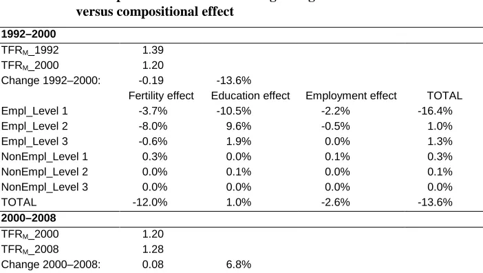
Table 3 is divided in three parts, one for each period examined. Each part can be read as follows: In 1992 the male TFR was 1.39, in 2000 it was 1.2, a change of -0.19 or -13.6%. During those years, the educational attainment was increasing, placing a growing number of men at higher education levels; the percentage of non-employed men also varied, influencing fertility decisions. All other things being equal, changes in educational patterns should have increased TFRM by 1%. Similarly, changes in employability should have lowered the fertility indicator by -2.6%. Thus, changes in TFRM during 1992–2000 are mostly behavioral rather than compositional, as they result from shifts in fertility rates, rather than variations by education level or employment status.
Table 3: Decomposition of factors affecting changes in TFR: behavioral versus compositional effect
1992–2000
TFRM_1992 1.39
TFRM_2000 1.20
Change 1992–2000: -0.19 -13.6%
Fertility effect Education effect Employment effect TOTAL
Empl_Level 1 -3.7% -10.5% -2.2% -16.4%
Empl_Level 2 -8.0% 9.6% -0.5% 1.0%
Empl_Level 3 -0.6% 1.9% 0.0% 1.3%
NonEmpl_Level 1 0.3% 0.0% 0.1% 0.3%
NonEmpl_Level 2 0.0% 0.1% 0.0% 0.1%
NonEmpl_Level 3 0.0% 0.0% 0.0% 0.0%
TOTAL -12.0% 1.0% -2.6% -13.6%
2000–2008
TFRM_2000 1.20
TFRM_2008 1.28
Table 3: (Continued)
2000–2008
Fertility effect Education effect Employment effect TOTAL
Empl_Level 1 -4.0% -2.7% 0.8% -5.9%
Empl_Level 2 7.5% 1.3% 0.5% 9.3%
Empl_Level 3 1.2% 2.0% 0.1% 3.4%
NonEmpl_Level 1 0.2% 0.0% -0.1% 0.0%
NonEmpl_Level 2 0.1% 0.0% -0.1% 0.0%
NonEmpl_Level 3 0.0% 0.0% 0.0% 0.0%
TOTAL 4.9% 0.6% 1.3% 6.8%
2008‒2011
TFRM_2008 1.28
TFRM_2011 1.15
Change 2008–2011: -0.13 -9.9%
Fertility effect Education effect Employment effect TOTAL
Empl_Level 1 0.4% -1.7% -4.7% -6.1%
Empl_Level 2 1.2% -0.2% -6.0% -5.0%
Empl_Level 3 -1.0% 2.0% -1.6% -0.6%
NonEmpl_Level 1 0.3% 0.0% 0.6% 0.9%
NonEmpl_Level 2 0.2% 0.0% 0.5% 0.7%
NonEmpl_Level 3 0.0% 0.0% 0.1% 0.1%
TOTAL 1.1% 0.0% -11.0% -9.9%
Moreover, the effect of each component can be further decomposed so as to estimate its impact on different educational groups (Level 1, 2 and 3) and the impact of employment status (employed, non-employed). Thus, in contrast to the overall TFR of the previously mentioned period (1992‒2000), fertility variations across less-educated employed men were driven mainly by compositional rather than behavioral changes. For this group (Empl_Level 1), TFR changed by -16.4%; this trend resulted mostly from distributional changes in educational levels and employability, -10.5% and -2.2% respectively, while fertility variations per se are limited to -3.7%.
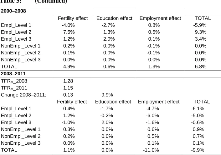
When read by columns, Table 3 shows the separate effect of fertility, education and employability on each and every population group per period. In certain cases, differentiations across population groups are noteworthy. For instance, despite being positive overall (1.1%), the fertility effect is negative (-1%) for highly educated employed men during the period 2008‒2011.
employed men falling in middle and upper education groups. Changes in employment rates had a positive effect on fertility for men of all education levels. During the years 2008 to 2011, decreasing employment was the chief factor to influence male fertility; this development exerted substantial downward pressure on TFRM (-11%) especially for men of low or middle level of education (-4.7% and -6.0% respectively).
4. Conclusion
In this study we investigated levels, trends, and differentials in male fertility, an issue scarcely addressed in the demographic literature. Based on Greek birth registrations for the years 1992 to 2011, we estimated male fertility rates and studied differences in fertility levels by education level and employment status. Moreover, using a decomposition method, we explored the distributional effect of educational attainment and employability on fertility outcomes.
Our findings indicate that, over the study period, the male fertility level is declining, the fertility pattern is ageing, and the reproduction period for men is getting shorter. Even though overall fertility declines for all educational groups, the decrease was by far more important among less educated men. As a consequence, and in sharp contrast to what was the norm until very recently, in 2011, the total fertility rate of well-educated men was by around 15% higher than that of men with a low education level. As for employment status, the fertility behavior of employed men is unquestionably the main component of the variations, over time, of total fertility. Nevertheless, it should not pass unnoticed that fertility among unemployed men is on the rise during the last years.
From 1992 up to 2008, changes in male fertility were mostly driven by behavioral rather than compositional factors (i.e., the variations over time in the distribution of male population by educational level and employment status). However, the role of the latter has become predominant since 2008: the decline of male fertility over the period 2008‒2011 is largely attributed to compositional effect, and in particular to the continuous decrease in the proportions of employed men. It could be assumed that this development reflects the impact of the economic recession and skyrocketing unemployment rates on fertility.
The lack of population data categorized by multiple characteristics is an essential limitation in demographic research. This simple approach, as described in the Appendix, suggests a way to overcome this shortcoming.
There are also some limitations. The most important one comes from the LFS itself; the sampling design, sample size and response rate are determinants that may undermine the reliability of produced data. The sample may suffer as we move away from the census years (used as basis for the sampling design), as concepts and definitions change with time, and as response rate varies. Certain population groups risk being under-represented, in the sample and the consistency of the results becomes questionable.
It would also be interesting to create a distinct category for the unemployed, instead of grouping them under the ‘non-employed’ label. In the context of economic downturn, shedding light on fertility outcomes of unemployed men would provide significant insights about how economic crisis and fertility are associated. Despite the availability of birth and population data on the unemployed, the choice made was not to proceed to such an exercise. Such a decision was dictated by the inconsistency in unemployment definition between vital statistics on births and LFS data. The former relies on self-declaration while the later attributes the status of “unemployed” under more specific time and duration criteria.
Findings suggest that male fertility is an important topic in the study of human reproduction that merits further exploration. Especially for years of economic downturn, and in countries where household living standards are mostly associated with male employment, fathers’ employment conditions are of increasing importance in shaping fertility outcomes. Further analysis of fertility seen from the male side would shed light on aspects that currently remain understudied, providing, for instance, more couple-level evidence on how employment uncertainties relate to fertility behavior, as well as to the timing and quantum of parenthood.
5. Acknowledgements
References
Adserà, A. (2004). Changing fertility rates in developed countries. The impact of labor market institutions. Journal of Population Economics 17: 17‒43. doi:10.1007/ s00148-003-0166-x.
Bachu, A. (1996). Fertility of American Men. Working Paper No 14. Washington, D.C.: Population Division.
Bagavos, C. (2003). Demographic Shifts, Labour Market and Pensions in Greece and in the European Union. Athens: Gutenberg: 406.
Bagavos, C. (2010). Education and childlessness: the relationship between educational field, educational level, employment and childlessness among Greek women born in 1955–1959. Vienna Yearbook of Population Research 8: 51‒75. doi:10.1553/populationyearbook2010s51.
Becker, S. (1999). Measuring unmet need: Wives, husbands or couples? International Family Planning Perspectives 25(4): 172‒180. doi:10.2307/2991881.
Bianchi, S.M. (1998). Introduction to the special issue: Men in families. Demography 36: 195‒203. doi:10.2307/2648108.
Bronte-Tinkew, J., Ryan, S., Franzetta, K., Manlove J., and Lilja, E. (2009). Higher-Order fertility Among Urban Fathers: An Overlooked Issue for a Neglected Population. Journal of Family Issues 30(7): 968‒1000. doi:10.1177/0192513X 08330947.
Brouard, N. (1977). Evolution de la fécondité masculine depuis le début du siècle. Population 32(6): 1123‒1158. doi:10.2307/1531392.
Coleman, D. (2000). Male fertility trends in industrial countries: Theories in search of some evidence. In: C. Bledsoe, J. Guyer, and S. Lerner (eds.). Fertility and male life-cycle in the era of fertility decline. New York: Oxford University Press: 1‒26.
Dodoo, N.-A. (1998). Men matter: Additive and interactive gendered preferences and reproductive behavior in Kenya. Demography 35(2): 229‒242. doi:10.2307/ 3004054.
Engelhardt, H. and Prskawetz, A. (2004). On the changing correlation between fertility and female employment over space and time. European Journal of Population 20: 35‒62. doi:10.1023/B:EUJP.0000014543.95571.3b.
European, Commission (1998). Demographic Report 1997. Annex B. Luxembourg: Office for Official Publications of the European Communities.
European, Commission (2012). Report from the Commission to the European Parliament and the Council on the implementation of Council Regulation (EC) No 577/98. COM(2012) 701 final.
Eurostat (2013a). Demography/Population on 1 January by age and sex. http://epp.eurostat.ec.europa.eu/portal/page/portal/statistics/search_database. Eurostat (2013b). LFS series-Detailed annual survey results, Population, aged 15 to 74
years, by sex, age and highest level of education attained (1000). http://epp.eurostat.ec.europa.eu/portal/page/portal/statistics/search_database. Eurostat (2013c). LFS series-Detailed annual survey results, Employment by sex, age
and highest level of education attained (1000). http://epp.eurostat.ec.europa.eu/ portal/page/portal/statistics/search_database.
Eurostat (2013d). Quality Report of the European Union Labour Force Survey. http://epp.eurostat.ec.europa.eu/cache/ITY_OFFPUB/KS-RA-13-008/EN/KS-RA-13-008-EN.PDF.
Fikree, F., Gray, R.H., and Shah, F. (1993). Can Men Be Trusted? A Comparison of Pregnancy Histories Reported by Husbands and Wives. American Journal of Epidemiology 138(4): 237‒242.
Forste, R. (2002). Where are all the men: a conceptual analysis of the role of men in family formation. Journal of Family Issues 23(5): 579‒600. doi:10.1177/0192 513X02023005001.
Greene, M.E. and Biddlecom, A.E. (2000). Absent and problematic men: demographic accounts of male reproductive roles.Population and Development Review 26(1): 81‒115. doi:10.1111/j.1728-4457.2000.00081.x.
Guzzo, K.B and Hayford, S.R. (2010). Single Mothers, Single Fathers: Gender Differences in Fertility After a Nonmarital Birth. Journal of Family Issues 3(7): 906‒933. doi:10.1177/0192513X09351508.
Juby, H. and Le Bourdais, C. (1999). Where have all the Children Gone? – Comparing Mothers’ and Fathers’ Declarations in Retrospective Surveys. Canadian Studies in Population 26(1): 1‒20.
Karanikoli, I. (2009). Issues related to the comparability of sampling surveys. The case of the LFS, 1998–2009. Panteion University, Departement of Social Policy. Kiernan, K.E. and Diamond, I. (1983). The age at which childbearing starts –a
longitudinal study. Population Studies 37(3): 363‒380. doi:10.2307/2174504. Kögel, T. (2004). Did the association between fertility and female employment within
OECD countries really change its sign? Journal of Population Economics 17: 45‒65. doi:10.1007/s00148-003-0180-z.
Kreyenfeld, M., Andersson, G., and Pailhé, A. (2012). Economic uncertainty and family dynamics in Europe. Special Collection 12. Demographic Research 27(28). 835‒852. doi:10.4054/DemRes.2012.27.28.
Lewis, C. and Ventura, S.J. (1990). Births and fertility rates by education. National Center for Health Statistics. Vital Health Statistics 21.
Lappegård, T. and Rønsen, M. (2013). Socioeconomic Differences in Multipartner Fertility Among Norwegian Men. Demography 50(3): 1135‒1153. doi:10.1007/s13524-012-0165-1.
Marciano, T.D. (1979). Male influences on fertility: Needs for research. The Family Coordination 28(4): 561‒568. doi:10.2307/583519.
Mott, F.L. and Mott, S.H. (1985). Household fertility decisions in West Africa: a comparison of male and female survey results. Studies in Family Planning 16(2): 88‒99. doi:10.2307/1965574.
Paget, W.J. and Timæus, I.M. (1994). A relational Compertz model of male fertility: development and assessment. Population Studies 48(2): 333‒340. doi:10.1080/ 0032472031000147826.
Poston, D.L.J. and Chang, C.-F. (2005). Bringing males in: A critical demographic plea for incorporating males in methodological and theoretical analyses of human fertility. Critical Demography 1(1): 1‒15.
Ravanera, Z. and Fernando, R. (2003). Fertility of Canadian Men: Levels, trends and correlates. PSC Discussion Papers Series 17(6): Article 1.
Rendall, M.S., Clarke, L., Peters, E., Rajnit, N., and Verropoulou, G. (1999). Incomplete reporting of men’s fertility in the United States and Britain: A research note. Demography 36(1): 135‒144. doi:10.2307/2648139.
Rendall, M., Aracil, E., Bagavos, C., Couet, C., Derose, A., Diqiulio, P., Lappegard T., Robert-Bobée, I., Rønsen, M., Smallwood, S., and Verropoulou, G. (2010). Increasingly heterogeneous ages at first birth by education in Southern European and Anglo-American family-policy regimes: A seven country comparison by birth control. Population Studies 64(3): 209‒227. doi:10.1080/00324728. 2010.512392.
Rindfuss, R., Morgan, P., and Offutt, K. (1996). Education and the changing age pattern of American fertility: 1963–1989. Demography 33(3): 227‒290. doi:10.2307/ 2061761.
Sobotka, T., Skirbekk, V., and Philipov, D. (2011). Economic Recession and Fertility in the Developed World. Population and Development Review 37(2): 267‒306. doi:10.1111/j.1728-4457.2011.00411.x.
Ventura, S.J., Martin, J.A., Curtin, S.C., Mathews, T.J., and Park, M.M. (2000). Births: Final data for 1998. National Vital Statistics Reports 48.
Yang, Y. and Morgan, S.P. (2003). How big are educational and racial differentials in the U.S.? Biodemography and Social Biology 50(3–4): 167‒187. doi:10.1080/ 19485565.2003.9989070.
Appendix A
Methodology used to estimate the male population by five-year age group, education level and employment status for non-census years. The approach uses annual EUROSTAT data on Demographic Statistics and Labor Force Surveys.
First Step:
♦ Data used in this step are from Eurostat-Demographic Statistics (2013a)
♦ Estimation of the average annual male population 𝑃�𝑥(t) per age
group (x) using the male population of the specific age group on January 1st of two consecutive years 𝑃
𝑥(𝑡) and 𝑃𝑥(𝑡+ 1): ♦ where,
♦ t: year (1992,…2011)
♦ x: five-year age group (0‒4, 5‒9, … , 80‒84, 85+)
Second Step:
♦ Data used in this step are from Eurostat-LFS (2013b)
♦ Calculation of proportion of male population 𝑎𝑥,𝑖 with
educational level (i) in each age group (x) per year:
♦ 𝑎𝑥,𝑖(𝑡) = 𝑃�𝑥,𝑖(𝑡)
∑ 𝑃�𝑖 𝑥,𝑖(𝑡)
♦ where,
♦ t: year (1992,…2011)
♦ i: educational level (i=1,2,3)
♦ x: five-year age group (0–4, 5–9, … , 80–84, 85+)
♦ 𝑃�𝑥,𝑖(𝑡): number of men of age x falling in educational level i.
Third Step:
♦ Estimation of the average male population by level of education at each age group (𝑃���𝑥,𝑖) per year, applying the proportions
calculated in step 2 (𝑎𝑥,𝑖) to the average population (𝑃�𝑥) as
estimated in step 1:
♦ 𝑃�𝑥,𝑖(𝑡) =𝑎𝑥,𝑖(𝑡)∗ 𝑃�𝑥(𝑡)
Fourth Step:
♦ Data used in this step are from Eurostat-LFS (2013c)
♦ Calculation of the employment rates (𝑝𝐸,𝑥,𝑖(𝑡)) for educational
♦ 𝑝𝐸,𝑥,𝑖(𝑡) =𝑃�𝐸,𝑥,𝑖(𝑡)
𝑃�𝑥,𝑖(𝑡)
Fifth Step:
♦ Estimation of the average employed 𝑃�𝐸,𝑥,𝑖(𝑡) and unemployed 𝑃�𝑁𝐸,𝑥,𝑖(𝑡) male population by age and level of education at year
t, applying the proportions calculated in step 4 (𝑝𝐸,𝑥,𝑖) to the average population (𝑃�𝑥,𝑖) by age and education level as
estimated in step 3:
♦ 𝑃�𝐸,𝑥,𝑖(𝑡) =𝑝𝐸,𝑥,𝑖(𝑡)∗ 𝑃�𝑥(𝑡)
♦ 𝑃�𝑁𝐸,𝑥,𝑖(𝑡) = (1− 𝑝𝐸,𝑥,𝑖(𝑡))∗ 𝑃�𝑥(𝑡)
Appendix B
− Construction of educational level variable
On the basis of the international standard classification of education (ISCED classification of 1997) three educational levels were used to describe this variable:
♦ Level 1: pre-primary, primary and lower secondary education (levels 0‒2),
♦ Level 2: upper secondary and post-secondary non-tertiary education (levels 3 and 4),
♦ Level 3: first and second stage of tertiary education (levels 5 and 6).
More precisely, in this work, Level 1 includes illiterates, those who know writing and reading, and persons with lower secondary education; Level 2 comprises all individuals with upper secondary education (post-secondary non-tertiary education is included at that level); Level 3 refers to people with a “diploma” which corresponds to first and second stage of tertiary education.