DEMOGRAPHIC RESEARCH
VOLUME 30, ARTICLE 65, PAGES 1769
−
1792
PUBLISHED 5 JUNE 2014
http://www.demographic-research.org/Volumes/Vol30/65/ DOI: 10.4054/DemRes.2014.30.65
Research Article
Homogamy in socio-economic background and
education, and the dissolution of cohabiting unions
Elina Mäenpää
Marika Jalovaara
©2014 Elina Mäenpää & Marika Jalovaara.
This open-access work is published under the terms of the Creative Commons Attribution NonCommercial License 2.0 Germany, which permits use, reproduction & distribution in any medium for non-commercial purposes, provided the original author(s) and source are given credit.
1 Introduction 1770
2 Background 1771
2.1 Hypotheses concerning the effects of homogamy on union stability 1771
2.2 Previous findings 1774
2.3 Measuring the effects of homogamy and heterogamy 1775
3 Data and method 1776
3.1 Data and study population 1776
3.2 Covariates 1777
3.3 Method and analytical strategy 1778
4 Results 1779
4.1 Homogamy in socio-economic background and cohabitation dissolution
1779
4.2 Homogamy in educational level and cohabitation dissolution 1781 4.3 The effects of the control variables 1783
5 Discussion 1784
6 Acknowledgements 1787
References 1788
Homogamy in socio-economic background and education, and the
dissolution of cohabiting unions
Elina Mäenpää1
Marika Jalovaara2
Abstract
BACKGROUND
Despite the increasing prevalence of cohabitation, knowledge of how socio-economic homogamy affects the stability of cohabiting unions is scant. Few studies have compared the effects of homogamy in both ascribed and achieved socio-economic status on union dissolution.
OBJECTIVE
Our aim is to determine how homogamy and heterogamy in educational level and parental social class affect the risk of cohabitation dissolution in Finland.
METHODS
We use unique Finnish register data that includes information on non-marital cohabitation. Cox regression is used to analyse the risk of dissolution in 20,452 cohabitations. We examine the dissolution rates in all possible combinations of partner status, and analyse how these estimates deviate from the main effects of each partner’s status.
RESULTS
According to the findings, homogamy in parental social class is of little consequence in cohabitation dissolution, although cohabitations between people from upper-white-collar and farmer families are disproportionately likely to dissolve. Educational differences between partners are more significant determinants of cohabitation stability: extreme heterogamy is associated with an increased separation risk, and homogamy decreases the separation risk among cohabitors with a higher university degree.
CONCLUSIONS
In line with the perception that personal achievement is more significant than social origins in contemporary union dynamics, similarity in educational level increases cohabitation stability more than similarity in socio-economic origin. Although previous Nordic studies report little or no association between educational homogamy or heterogamy and marriage dissolution, our study shows that educational differences do matter in cohabiting unions.
1. Introduction
The extent to which socio-economic homogamy – in other words, similarity in partner status – guides union formation and dissolution is considered an indicator of barriers between status groups in a society. A strong homogamy tendency in partner selection and a disproportionate likelihood of union disruption among heterogamous couples may point to large social and cultural gaps between socio-economic groups. This study explores the effects of homogamy and heterogamy in educational level and parental social class on union dissolution in Finland. The aim is to assess the significance of status differences for union stability, and to determine whether similarity in childhood socio-economic circumstances or the achieved position of the partners is more decisive in contemporary union dynamics. Few studies thus far compare the effects of homogamy in ascribed and achieved socio-economic position on union stability. Research on partner selection nevertheless indicates that homogamy in achieved status is more prominent than in ascribed status (Kalmijn 1991, 1998; Hansen 1995). However, tendencies in partner selection result not only from people’s preferences but also from the structural opportunities to meet and interact with potential partners of a similar status. One means of eliminating the effect of these structural factors is to examine the decisions the partners make after they have formed the union, such as to separate (see Hansen 1995; Müller 2003). Examining the effects of homogamy and heterogamy on union dissolution may thus facilitate assessment of whether people actually prefer partners who share similar socio-economic characteristics.
it is estimated that within ten years of formation, less than 40% of cohabitations have been converted to marriages, and over 50% are dissolved (Jalovaara 2013). Given that separation rates in Finland are known to be higher in cohabiting unions than in marriages (Liefbroer and Dourleijn 2006; Jalovaara 2013), dissolving unions are highly likely to be cohabitations. However, even in the Nordic countries research on union dissolution has focused mainly on marriages, and therefore little is known about the antecedents of cohabitation dissolution. The excellent Finnish register data enables us to fill this gap in knowledge regarding how socio-economic homogamy affects the stability of non-marital cohabitations.
Our study extends previous research on the effects of homogamy and heterogamy on union stability in several other ways as well. First, we examine the effects of homogamy in both parental social class (ascribed status) and individual educational attainment (achieved status). Numerous studies have investigated the effects of educational differences between partners on divorce risk, but less is known about the effects of homogamy in socio-economic origins on union stability. Second, given that homogamy is normative in unions, heterogamous couples tend to be rare, and studying them requires extensive data. The large number of observations in the register data at our disposal enables us to examine the probability of union dissolution in each combination of partner status, and thus to analyse the infrequent but theoretically interesting heterogamous couples, as well as different kinds of homogamous couples. These analyses produce exceptionally detailed knowledge about the effects of social boundaries on union stability. Finally, the use of register data allows us to avoid many of the problems encountered in studies based on survey data, such as biased samples due to the self-selection of respondents, and the misreporting of partner characteristics.
2. Background
2.1 Hypotheses concerning the effects of homogamy on union stability
Janssen 2005). We thus expect homogamy in socio-economic background and educational level to increase, and heterogamy to decrease union stability (H1).
Individuals’ values, tastes, and lifestyles are shaped both within the parental family environment and in contexts outside it, such as in educational institutions and peer groups (Kalmijn 1991; Hansen 1995). If early socialization is particularly significant in the formation of cultural resources, homogamy in ascribed characteristics such as parental social class and ethnic background should diminish the risk of union dissolution (Hansen 1995). Social support from parental families and social networks may further increase union stability (Janssen 2002; Kalmijn, de Graaf, and Janssen 2005). On the other hand, if orientations and influences later in life (e.g., educational institutions and peer groups) strongly shape values and lifestyles, homogamy in achieved characteristics such as educational level and occupation should be decisive in terms of union stability (Hansen 1995). Existing literature postulates that as intergenerational social mobility has increased and young adults have become increasingly independent of their parents, social origin has become less important than achieved status in partner-selection decisions (Kalmijn 1991, 1998; Hansen 1995). Education in particular is considered to have a strong effect on the cultural resources of individuals, and hence on their partner preferences (Kalmijn 1991, 1998; Hansen 1995; Blossfeld 2009). On these grounds we posit that educational homogamy is more important than homogamy in socio-economic background in maintaining union stability (H2).
Given that the unions investigated in this study are cohabitations rather than marriages, similarity in achieved status is all the more likely to be of greater significance for their stability than similarity in ascribed status. The level of commitment among cohabiting couples is perceived as being lower than among married couples, indicated for instance in the higher dissolution rates (Liefbroer and Dourleijn 2006; Jalovaara 2013), lower childbearing intensity (Oláh and Bernhardt 2008), and more frequent break-up plans (Wiik, Bernhardt, and Noack 2009) among cohabitors. It has been suggested that cohabitors are therefore less concerned with kinship issues and more loosely bound to the wider family network than married partners (Schoen and Weinick 1993). This implies that homogamy in ascribed characteristics, such as social origins, is less relevant for cohabiting than for married couples (ibid.).
which the male partner is more highly educated than the female partner) compared with homogamous couples. A union-stabilizing effect of educational hypergamy is unlikely to appear in the current study, however, for at least two reasons. First, given the high level of education and labour-force-participation rate among women in Finland, and the fact that the dual-earner family has become the social standard, economic dependence between partners is likely to be relatively symmetrical. Second, as noted in the literature, cohabiting partners in particular are likely to stay together under conditions of equality. Because cohabitation is often short-lived, and cohabiting partners have no legal marriage contract to secure them in case of a break-up (Brines and Joyner 1999), and also because there are fewer norms regarding the roles and behaviour of cohabiting rather than marriage partners (Baxter 2005), cohabitors tend to be more averse than married couples to the gendered division of household labour. Empirical evidence has shown that both attitudes and the actual division of housework are indeed more gender-egalitarian among cohabitors than among married couples (Smock 2000; Baxter 2005; Davis, Greenstein, and Gerteisen Marks 2007; Domínguez-Folgueras 2013). Accordingly, it has been suggested that socio-economic equality rather than specialization promotes cohabitation stability (Brines and Joyner 1999; Kalmijn, Loeve, and Manting 2007; Jalovaara 2013).
Given that our data enables us to examine the risks of union dissolution in each partner combination, we extend the general heterogamy hypothesis and posit that the effects of homogamy and heterogamy may depend on the social stratum. In accordance with the notion that homogamy in social origins is a means of maintaining class cultures and keeping distances between social groups, it has been argued that in-group union formation is particularly important for the upper classes of a society because it helps them to retain their privileged position (Hansen 1995). We thus assume that
2.2 Previous findings
Few studies examine how educational differences between cohabiting partners affect their probability of separating. Nevertheless, those that have been conducted indicate that educational heterogamy does play a role in cohabitation stability: Brown (2000) found that heterogamous couples in the U.S. faced an increased separation risk relative to homogamous couples, although the effect was not statistically significant, and Smock and Manning (1997) reported an elevated risk among clearly hypergamous couples. Moreover, educational hypogamy has been reported to increase the probability of cohabitation dissolution in West Germany (Müller 2003). The effects of educational differences on cohabitation stability have not been examined in the Nordic countries so far, but results concerning marriage dissolution in these countries are not supportive of the general heterogamy hypothesis: educational heterogamy has been reported to have only a minor (Jalovaara 2003) or no impact on divorce risk (Hansen 1995; Finnäs 1997; Lyngstad 2004, 2006). More clearly evident divorce-promoting effects of educational heterogamy have been observed in the U.S. and Western Europe, however (Bumpass, Castro Martin, and Sweet 1991; Tzeng 1992; Heaton 2002; Schoen 2002; Schoen et al. 2002; Kalmijn 2003; Müller 2003).
Studies examining the effects of homogamy in socio-economic family background on union dissolution are few and far between, which is probably due to the lack of data on both partners’ parental family characteristics. Contradicting the hypothesis that homogamy in achieved socio-economic status is more important for union stability than homogamy in socio-economic origin, a Norwegian study (Hansen 1995) found that homogamy with respect to paternal occupational class rather than educational homogamy decreased divorce risk. Distinguishing between the economic and cultural aspects of paternal occupational status, Janssen (2002) found that homogamy in economic social origin, but not in cultural social origin, decreased the probability of divorce in the Netherlands. To the best of our knowledge, there have been no studies on the effects of homogamy in socio-economic family background on cohabitation dissolution.
more strongly than the formation of a cohabiting union (Jalovaara 2012), and some of the union-stabilizing effects of greater socio-economic resources were stronger in marriages than in cohabitations (Jalovaara 2013). The female partner’s higher contribution to household income was found to encourage separation in both union types: in the case of cohabitation this only happened when the woman’s income clearly exceeded that of her partner, whereas the effect was stronger and more consistent in marriages (Jalovaara 2013). A previous paper based on the same study population as the current study shows how homogamy and heterogamy in socio-economic origin and educational level affect the probability that a cohabiting couple will proceed from cohabitation to marriage (Mäenpää and Jalovaara 2013). The results indicate that homogamous couples are not selected from cohabitation to marriage to any great extent in Finland: homogamy increased the marriage rate only among people who grew up in farmer families and those with no more than a basic level of education. Another significant finding was that the effects of educational heterogamy on the transition to marriage were not unequivocal, but varied across educational combinations of partners. What has not yet been studied is how similarity and dissimilarity in cohabiting partners’ educational attainments and socio-economic family background influence their propensity to separate. This is the aspect we focus on in this paper.
2.3 Measuring the effects of homogamy and heterogamy
3. Data and method
3.1 Data and study population
The data are extracted from the so-called Palapeli research register compiled at Statistics Finland. The register covers all individuals who belonged to the population of Finland on 31 December in at least one of the years between 1970 and 2000, and was formed by linking data from the population register and census and employment statistics, for instance, by means of personal identity codes. Palapeli comprises information on individuals and all their unions, partners, and children up to December 2003. Data on the partners’ demographic and socio-economic characteristics are symmetrical, which is a major advantage in the study of homogamy. The extract analysed here is an 11% sample of individuals born before 1986.
Exceptionally, Palapeli includes detailed data on cohabiting unions from 1987 onwards. Unlike registers in Sweden and Norway, which identify cohabiting unions only when the couple has shared children, the Finnish registration system enables the inference of all cohabitations because a person’s place of residence is known to the precision of a dwelling. Cohabiting couples are defined in Palapeli as a male and a female who have been domiciled in the same dwelling for over 90 days, who are not married to each other, who have no more than a 20-year age difference (this rule does not apply if the couple has shared children), and who are not siblings, or a parent and a child. The dates of union formation and dissolution are precise within one month.
We analysed cohabiting unions formed by women born in 1960–1977 during the period from January 1995 to December 2002. During this period 24,823 women entered a cohabiting union. Among those who had formed more than one such union the first one was included in the analysis. Only unions in which both partners were born in Finland were included in the study because much of the data on individuals born abroad are deficient with regard to the time preceding immigration. This condition excluded 1,921 cohabitations. Women whose partner was born before 1956 were also excluded (n
= 1,039) because parental occupational class can be inferred only for birth cohorts from 1956 onwards. Furthermore, because many people under 20 years of age are still in education, unions formed when the women were under the age of 20 were excluded (n
= 1,615). The final number of cohabiting unions was 20,452.
observation period ended (December 2003). During the follow-up, cohabitations contributed 674,316 months at risk. In total 7,463 cohabiting couples (36.5%) separated, 6,448 (31.5%) married, 76 (0.4%) were censored through migration or death, and 6,465 (31.6%) were still cohabiting in December 2003.
3.2 Covariates
We measured socio-economic background in terms of parental occupational class.3 This can be inferred from data on each person below the age of 15, when the household’s reference person determines the occupational class. The reference person is the individual who is interpreted as having the primary responsibility for the subsistence of the household. In practice it is the parent with the higher income, and hence in most two-parent families it is the father. Occupational class is given in the register for every fifth year since 1970, and the measures were taken when the partners were 8–14 years old, depending on their year of birth. The first three categories distinguish people from (1) upper-white-collar employee families, (2) lower-white-collar employee families and (3) blue-collar families. The fourth group comprises people who grew up in farmer families (4). This category is qualitatively important in the case of Finland, which industrialized relatively late. The country is geographically and also socio-culturally quite strongly divided into urban areas on the one hand and sparsely populated countryside on the other. ‘Farmer’ here refers to self-employed people and employers in agriculture, forestry, and fishing, workers in these fields being classified as blue-collar workers. 15% of the Finnish labour force worked in agriculture, forestry, and fishing in 1975, and around half of them were self-employed workers without employees (Statistics Finland 1981). The last category is the residual group ‘Other’ (5), and includes individuals whose parental occupational status is student or pensioner, as well as those for whom data is missing. Individuals originating from families of self-employed people and employers (other than farmers) are also placed in this category: the data does not distinguish between small entrepreneurs and owners of large companies; thus the group would not constitute a meaningful category in itself. Self-employed people and employers comprise about half of the category, on account of which it is heterogeneous, and the results are not easy to interpret. Appendix Table 1 shows the months at risk by the partners’ parental occupational classes.
3 Using parental education instead of occupational class would yield a more symmetrical measurement of
Given that Palapeli provides month-level data on the completion of educational qualifications, we constructed monthly updated time-varying covariates depicting the partners’ educational levels (lagged one month). Individuals with no registered post-comprehensive, non-compulsory education are interpreted as having a basic-level qualification (1), which means at most nine years of education. Education up to the upper-secondary level (2) lasts 11–12 years and includes the matriculation examination (i.e., the final examination at the end of upper-secondary school that yields eligibility for higher education) and vocational qualifications obtained in one to three years. Lower-tertiary education (3) includes the lowest level of tertiary study (2–3 years following the upper-secondary level) and the lower-degree level (3–4 years following the upper-secondary level, e.g., polytechnic degrees and Bachelor’s degrees from universities). Upper-tertiary education (4) includes the higher-degree level (5–6 years following upper-secondary education, e.g., Master’s degrees from universities), as well as doctorates or equivalent education. Appendix Table 2 shows months at risk by the partners’ educational levels.
We controlled for four basic factors that could have distorted our analysis of the association between socio-economic homogamy and union dissolution. Seven categories of age homogamy are distinguished: (1) female 8 or more years older, (2) female 4–<8 years older, (3) female >0–<4 years older, (4) male 0–<4 years older, (5) male 4–<8 years older, (6) male 8–<12 years older, and (7) male 12 or more years older. The female partner’s age at cohabitation entry is classified in five categories: (1) 20–24, (2) 25–29, (3) 30–34, (4) 35–39, and (5) 40–42. A couple’s place of residence is a time-varying covariate indicating where they resided at the end of the previous calendar year, updated yearly and categorized as follows: (1) Helsinki metropolitan area, (2) other urban, (3) semi-urban, and (4) rural. Parental status is a time-varying covariate, updated monthly and lagged one month. We formed seven categories (see Table 5) according to whether the couple had shared children, whether the child was the couple’s first or a later child, whether the woman was pregnant, and whether the child was 0–12 months old or older. Pregnancy was deduced from the registered birth dates, and defined as seven months preceding a birth. The months at risk according to the control variables are shown in Table 5.
3.3 Method and analytical strategy
effects of the male and the female partners’ statuses on the risk of cohabitation dissolution. In the joint-effects model the full interaction of the partners’ statuses is considered. For both socio-economic background and educational level the full interaction models produced a statistically significant improvement in fit. We then examined the parameter estimates in each cell and compared them with the estimates of the main-effects model to identify the forms of homogamy and heterogamy that decrease or increase the risk of dissolution.
When we analysed the main effects and the joint effects of the partners’ parental occupational classes we controlled for the joint effects of their educational levels, and vice versa, in order to determine the independent effects of these two dimensions of homogamy. The control variables introduced above are also included in all the models.
4. Results
4.1 Homogamy in socio-economic background and cohabitation dissolution
Table 1 gives the main effects of parental occupational class on the risk of cohabitation dissolution. Among the women, separation risk is somewhat lower among those from farmer families than among other groups. No marked differences by socio-economic background are observable among the men.
The estimates in Table 2 are from fully adjusted models. The same interactive effects nevertheless emerge without adjusting for the four control variables as well (results not shown). In addition, the estimates from the joint-effects model of parental occupational class are practically the same regardless of whether we control only for the main effects of the partners’ educational levels, or also their joint effects. Similarly, the effects of educational differences (Table 4) are robust to the inclusion of the interaction of the partners’ parental occupational classes in the model. Homogamy in educational level and parental social class thus affect the likelihood of dissolving a cohabiting union independently of one another.
Table 1: The main effects of parental occupational class on the risk of
cohabitation dissolution, hazard ratios (HR) from a Cox regression model
Parental occupational class Female partner Male partner
Upper white collara 1.00 1.00
Lower white collar 0.97 0.95
Blue-collar worker 0.93* 0.98
Farmer 0.86** 0.97
Other 1.00 1.05
Note: The hazard ratios are adjusted for the control variables in Table 5 and the joint effects of educational level. *p < .05. **p < .01. ***p < .001.
a
Reference category.
Source: Palapeli register data, cohabitations formed during 1995–2002 involving women born in 1960–1977.
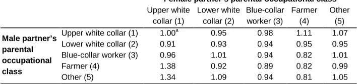
Table 2: The joint effects of parental occupational class on the risk of
cohabitation dissolution, hazard ratios (HR) from a Cox regression model
Female partner’s parental occupational class
Upper white collar (1)
Lower white collar (2)
Blue-collar worker (3)
Farmer (4)
Other (5)
Male partner’s parental occupational class
Upper white collar (1) 1.00a 0.95 0.98 1.11 1.07 Lower white collar (2) 0.91 0.93 0.94 0.95 0.95 Blue-collar worker (3) 0.96 1.01 0.94 0.82 1.01
Farmer (4) 1.38 0.92 0.89 0.82 0.99
Other (5) 1.34 1.09 0.94 0.81 1.05
Note: The hazard ratios are adjusted for the control variables in Table 5, and the joint effects of educational level.
a
Reference category.
4.2 Homogamy in educational level and cohabitation dissolution
Table 3 presents the main effects of educational level. Among both women and men, higher educational attainment is associated with a reduced probability of cohabitation dissolution: individuals with only a basic-level education stand out as being at the highest risk of separation, whereas the risk is lowest among those with a tertiary-level education. A negative educational gradient has also been reported for both sexes in previous Nordic studies on cohabitation dissolution (Jalovaara 2013) and divorce from marriage (e.g., Finnäs 1997; Jalovaara 2001, 2003, 2013; Lyngstad 2004, 2006, 2011).
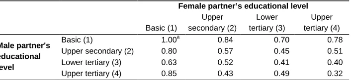
Model fit comparison indicates that the full interaction between the partners’ educational levels is statistically significant (p = 0.004). As Table 4 shows, the hazard ratios from the joint-effects model often diverge from the main effects given in Table 3. Apparent deviations are found among couples in which one partner has a basic-level education (column 1 and row 1 in Table 4). A large educational difference increases the probability of cohabitation dissolution: the main-effects model predicts men with an upper-tertiary education to have a 43% lower separation risk than men with a basic-level education across all educational basic-levels of the woman, while the joint-effects model estimates that if the female partner is educated to the basic level (column 1) the reduction is only 15%. While the main-effects model predicts upper-tertiary educated women to have a 38% lower separation risk than basic-level educated women across all levels of partner’s education, if the male partner has no education beyond the basic level (row 1) the advantage in stability is only 22%.
Less extreme forms of educational heterogamy do not appear to substantially elevate the separation risk. Among people with an upper-secondary level education (column 2 and row 2) differences in separation risks by the partner’s educational attainment are not very different from the estimates of the main-effects model. One interactive effect emerges among those with a lower-tertiary education (column 3 and row 3): while the main-effects model predicts upper-tertiary educated men to have a 43% lower separation risk than men with a basic-level education across all levels of the woman’s education, if the female partner is educated to the lower-tertiary level (column 3) the reduction is only 30% (1-(0.49/0.70)).
separation rate by 38%, 19% (1-(0.62/0.77)), and 2% (1-(0.62/0.63)) compared with basic, upper-secondary, and lower-tertiary education, respectively, but if the male partner is educated to the upper-tertiary level (row 4) the reductions are as much as 62% (1-(0.32/0.85)), 26% (1-(0.32/0.43)), and 35% (1-(0.32/0.49)).
The results concerning the effects of educational differences on cohabitation dissolution are also very robust to the adjustment of the four control variables (results not shown). However, among couples who are extremely hypogamous with respect to education (those in which the male is educated to the basic and the female to the upper-tertiary level), there is some ‘excess’ risk of separation that is attributable to age heterogamy: if we did not control for age homogamy, the dissolution-promoting effect of educational hypogamy would be even greater than in the fully adjusted model displayed above.
Table 3: The main effects of educational level on the risk of cohabitation
dissolution, hazard ratios (HR) from a Cox regression model
Educational level Female partner Male partner
Basica 1.00 1.00
Upper secondary 0.77*** 0.70***
Lower tertiary 0.63*** 0.61***
Upper tertiary 0.62*** 0.57***
Notes: Educational levels are time-varying covariates. The hazard ratios are adjusted for the control variables in Table 5 and the joint effects of parental occupational class.
*p < .05. **p < .01. ***p < .001.
a
Reference category.
Source: As for Table 1.
Table 4: The joint effects of educational level on the risk of cohabitation
dissolution, hazard ratios (HR) from a Cox regression model
Female partner’s educational level
Basic (1)
Upper secondary (2)
Lower tertiary (3)
Upper tertiary (4)
Male partner's educational level
Basic (1) 1.00a 0.84 0.70 0.78
Upper secondary (2) 0.80 0.57 0.45 0.51
Lower tertiary (3) 0.63 0.52 0.41 0.40
Upper tertiary (4) 0.85 0.43 0.49 0.32
Notes: The combined variable is a time-varying covariate. The hazard ratios are adjusted for the control variables in Table 5 and the joint effects of parental occupational class.
a
Reference category.
4.3 The effects of the control variables
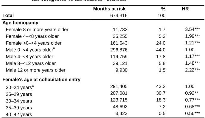
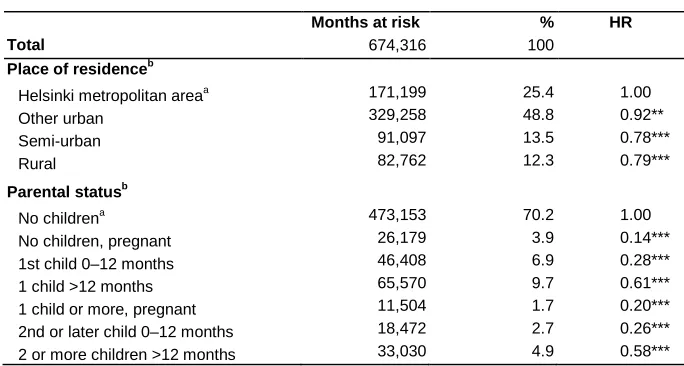
Table 5 shows the effects of the control variables on the risk of cohabitation dissolution. The greater the difference between the partners’ ages the higher the probability of separation. The gradient is steeper when the female partner is older, which conforms with previous Nordic findings that age heterogamy increases divorce risk especially when the wife is older (Hansen 1995; Finnäs 1997; Lyngstad 2004). The female partner’s age at cohabitation entry is negatively associated with the risk of dissolution. This could indicate that cohabitations formed at younger ages are more likely to be ‘trial marriages’ or less serious relationships that might be comparable to going steady rather than marriage, whereas those formed at later ages are more likely to be social substitutes for marriage. The separation rate is lower among couples residing in semi-urban and rural municipalities than among those residing in semi-urban areas. Not surprisingly, pregnancy and parenthood are associated with a reduced risk of cohabitation dissolution. Dissolutions are very rare during pregnancy and the child’s first year, but the risk increases as the children grow. Overall, the effects of the control variables correspond with the findings of previous studies on union dissolution (see Lyngstad and Jalovaara 2010).
Table 5: Months at risk and hazard ratios of cohabitation dissolution (HR) in
the categories of the control variables
Months at risk % HR
Total 674,316 100
Age homogamy
Female 8 or more years older 11,732 1.7 3.54***
Female 4–<8 years older 35,255 5.2 1.99***
Female >0–<4 years older 161,643 24.0 1.21***
Male 0–<4 years oldera 296,876 44.0 1.00
Male 4–<8 years older 119,759 17.8 1.17***
Male 8–<12 years older 39,121 5.8 1.48***
Male 12 or more years older 9,930 1.5 2.22***
Female's age at cohabitation entry
20–24 yearsa 291,405 43.2 1.00
25–29 years 207,081 30.7 0.92**
30–34 years 123,715 18.3 0.77***
35–39 years 48,692 7.2 0.68***
Table 5: (Continued)
Months at risk % HR
Total 674,316 100
Place of residenceb
Helsinki metropolitan areaa 171,199 25.4 1.00
Other urban 329,258 48.8 0.92**
Semi-urban 91,097 13.5 0.78***
Rural 82,762 12.3 0.79***
Parental statusb
No childrena 473,153 70.2 1.00
No children, pregnant 26,179 3.9 0.14***
1st child 0–12 months 46,408 6.9 0.28***
1 child >12 months 65,570 9.7 0.61***
1 child or more, pregnant 11,504 1.7 0.20***
2nd or later child 0–12 months 18,472 2.7 0.26***
2 or more children >12 months 33,030 4.9 0.58***
Notes: The hazard ratios are adjusted for other covariates in the table, the joint effects of parental occupational class, and the joint effects of educational level.
*p < .05. **p < .01. ***p < .001.
a
Reference category.
b
Time-varying covariate.
Source: As for Table 1.
5. Discussion
The purpose of this study was to examine the effects of homogamy and heterogamy in socio-economic background and educational attainment on the risk of cohabitation dissolution. We used unique Finnish register data offering a large number of observations that enabled the analysis of dissolution risks in all possible combinations of partner status. After confirming the statistical significance of the full interaction between the partners’ statuses, we identified the forms of homogamy and heterogamy that influenced the propensity to separate by examining in which cases the estimates from the joint-effects model deviated from the main effects of the female and the male partners’ statuses.
and the other came from an upper-white-collar family. Hence, our hypothesis that homogamy would contribute to union stability among people from upper-white-collar families in particular (H3) is only weakly supported. The increased dissolution risk of unions between people from upper-white-collar families and farmer families is nevertheless consistent with the assumption that heterogamy is more likely to undermine union stability when the cultural distance between the groups is large (H4). The dissolution rate of cohabitations in which the female came from an upper-white-collar family and the male from the residual category ‘Other’ was also higher than might be expected on the basis of the main effects, but this effect did not apply when the genders were reversed.
Educational homogamy turned out to be relatively more important for cohabitation stability than homogamy in socio-economic family background. Extreme educational heterogamy – one partner having no education beyond the basic level and the other having a higher university degree – was clearly associated with an increased propensity to separate. This is in line with the hypothesis that a large educational difference in particular decreases cohabitation stability (H4). The separation risk of heterogamous couples in which the female was educated to the lower-tertiary level and the male to the upper-tertiary level was also higher than implied by the main effects. The general heterogamy hypothesis thus seems to apply particularly to the highest educated cohabitors: all the dissolution-promoting effects of heterogamy involve cohabitors with a higher university degree, and homogamy substantially reduced the dissolution risk among this group. This finding could suggest that the highest educated are most distinct from other groups in terms of values and lifestyles. As we expected, educational hypergamy did not reduce the risk of cohabitation dissolution: on the contrary, the dissolution-promoting effect of extreme hypergamy was even more notable than the respective effect of extreme hypogamy. The results are thus in accordance with the view that equal socio-economic contributions rather than male socio-economic dominance enhance cohabitation stability. Overall, we can say that educational differences between cohabiting partners affect the probability of separation more consistently than they affect the probability of proceeding to marriage (cf. Mäenpää and Jalovaara 2013).
they might not be willing to marry. Heterogamous cohabiting couples in particular might be less seriously involved in the relationship, which could explain their increased propensity to split up. On the other hand, heterogamous couples that marry might be especially committed to the relationship and have very serious intentions, which relates to a low probability of breaking up. Other kinds of processes behind selection from cohabitation to marriage may also play a role. Although educationally heterogamous couples are not ‘weeded out’ to any significant extent in the transition from cohabitation to marriage in Finland (Mäenpää and Jalovaara 2013), which could attenuate the effects of educational differences in marriages, it could be that the couples who marry have certain unobserved characteristics (such as personality traits or socio-economic attributes other than educational level) that render educational differences between them inconsequential in terms of marital stability. The extent to which the difference in the effects of educational heterogamy on cohabitation and marriage stability is attributable to union type per se as opposed to selection effects is a question for future research.
In line with hypothesis H2, our findings show that similarity with respect to individual educational attainment is a more important factor in cohabitation stability than similarity with respect to socio-economic family background. The scant effects of parental social class and the greater significance of education found here – in terms of both the main effects and the interactions between the partners’ statuses – comply with the general conception that in modern, individualized societies one’s own orientations and achievements influence one’s life course more strongly than one’s ascribed socio-economic status (Treiman and Yip 1989; Hansen 1995). The effects of social origin on life-course outcomes may be particularly weak in a country such as Finland, in which several state policies (such as tuition-free education up to the university level) aim at providing equal opportunities for citizens irrespective of their social background. Accordingly, the association between ascribed and achieved socio-economic status is reported to be comparatively weak in the Nordic countries (Breen and Jonsson 2005; Pfeffer 2008; Katrňák, Fučík, and Luijkx 2012).
6. Acknowledgements
References
Baxter, J. (2005). To marry or not to marry: marital status and the household division of labor. Journal of Family Issues 26(3): 300–321. doi:10.1177/0192513X0427 0473.
Becker, G.S., Landes, E.M., and Michael, R.T. (1977). An economic analysis of marital instability. Journal of Political Economy 85(6): 1141–1187. doi:10.1086/ 260631.
Blossfeld, H.-P. (2009). Educational assortative marriage in comparative perspective.
Annual Review of Sociology 35: 513–530. doi:10.1146/annurev-soc-070308-11 5913.
Breen, R. and Jonsson, J.O. (2005). Inequality of opportunity in comparative perspective: Recent research on educational attainment and social mobility.
Annual Review of Sociology 31: 223–243. doi:10.1146/annurev.soc.31.041304. 122232.
Brines, J. and Joyner, K. (1999). The ties that bind: principles of cohesion in cohabitation and marriage. American Sociological Review 64(3): 333–355.
doi:10.2307/2657490.
Brown, S.L. (2000). Union transitions among cohabitors: the significance of relationship assessments and expectations. Journal of Marriage and the Family
62(3): 833–846. doi:10.1111/j.1741-3737.2000.00833.x.
Bumpass, L.L., Castro Martin, T., and Sweet, J.A. (1991). The impact of family background and early marital factors on marital disruption. Journal of Family Issues 12(1): 22–42. doi:10.1177/019251391012001003.
Bumpass, L.L. and Sweet, J.A. (1972). Differentials in marital instability: 1970.
American Sociological Review 37(6): 754–766. doi:10.2307/2093585.
Davis, S.N., Greenstein, T.N., and Gerteisen Marks, J.P. (2007). Effects of union type on division of household labor. Do cohabiting men really perform more housework? Journal of Family Issues 28(9): 1246–1272. doi:10.1177/ 0192513X07300968.
Eeckhaut, M.C.W., Van de Putte, B., Gerris, J.R.M., and Vermulst, A.A. (2013). Analysing the effect of educational differences between partners: a methodological/theoretical comparison. European Sociological Review 29(1): 60–73. doi:10.1093/esr/jcr040.
Finnäs, F. (1997). Social integration, heterogeneity, and divorce: the case of the Swedish-speaking population in Finland. Acta Sociologica 40(3): 263–277. Hansen, M.N. (1995). Class and Inequality in Norway. The Impact of Social Class
Origin on Education, Occupational Success, Marriage and Divorce in the Post-War Generation. Oslo: Institute for Social Research.
Heaton, T.B. (2002). Factors contributing to increasing marital stability in the United States. Journal of Family Issues 23(3): 392–409. doi:10.1177/0192513X02023 003004.
Heuveline, P. and Timberlake, J.M. (2004). The role of cohabitation in family formation: the United States in comparative perspective. Journal of Marriage and Family 66(5): 1214–1230. doi:10.1111/j.0022-2445.2004.00088.x.
Jalovaara, M. (2001). Socio-economic status and divorce in first marriages in Finland 1991–93. Population Studies 55(2): 119–133. doi:10.1080/00324720127685. Jalovaara, M. (2003). The joint effects of marriage partners’ socio-economic positions
on the risk of divorce. Demography 40(1): 67–81. doi:10.1353/dem.2003.0004. Jalovaara, M. (2012). Socio-economic resources and first-union formation in Finland,
cohorts born 1969–81. Population Studies 66(1): 69–85. doi:10.1080/ 00324728.2011.641720.
Jalovaara, M. (2013). Socioeconomic resources and the dissolution of cohabitations and marriages. European Journal of Population 29(2): 167–193. doi:10.1007/ s10680-012-9280-3.
Janssen, J.P.G. (2002). Do Opposites Attract Divorce? Dimensions of Mixed Marriage and the Risk of Divorce in the Netherlands. Nijmegen: ICS-dissertation.
Kalmijn, M. (1991). Status homogamy in the United States. American Journal of Sociology 97(2): 496–523. doi:10.1086/229786.
Kalmijn, M. (2003). Union disruption in the Netherlands: opposing influences of task specialization and assortative mating? International Journal of Sociology 33(2): 36–64.
Kalmijn, M., de Graaf, P.M., and Janssen, J.P.G. (2005). Intermarriage and the risk of divorce in the Netherlands: the effects of differences in religion and in nationality, 1974–94. Population Studies 59(1): 71–85. doi:10.1080/ 0032472052000332719.
Kalmijn, M., Loeve, A., and Manting, D. (2007). Income dynamics in couples and the dissolution of marriage and cohabitation. Demography 44(1): 159–179.
doi:10.1353/dem.2007.0005.
Katrňák, T., Fučík, P. and Luijkx, R. (2012). The relationship between educational homogamy and educational mobility in 29 European countries. International Sociology 27(4): 551–573. doi:10.1177/0268580911423061.
Kiernan, K. (2001). The rise of cohabitation and childbearing outside marriage in Western Europe. International Journal of Law, Policy and the Family 15(1): 1– 21. doi:10.1093/lawfam/15.1.1.
Liefbroer, A.C. and Dourleijn, E. (2006). Unmarried cohabitation and union stability: testing the role of diffusion using data from 16 European countries. Demography
43(2): 203–221. doi:10.1353/dem.2006.0018.
Lyngstad, T.H. (2004). The impact of parents’ and spouses’ education on divorce rates in Norway. Demographic Research 10(5): 121–142. doi:10.4054/DemRes.2004. 10.5.
Lyngstad, T.H. (2006). Why do couples with highly educated parents have higher divorce rates? European Sociological Review 22(1): 49–60. doi:10.1093/esr/ jci041.
Lyngstad, T.H. (2011). Does community context have an important impact on divorce risk? A fixed-effects study of twenty Norwegian first-marriage cohorts.
European Journal of Population 27(1): 57–77. doi:10.1007/s10680-010-9226-6. Lyngstad, T.H. and Jalovaara, M. (2010). A review of the antecedents of union
dissolution. Demographic Research 23(10): 257–291. doi:10.4054/DemRes. 2010.23.10.
Mäenpää, E. and Jalovaara, M. (2013). The effects of homogamy in socio-economic background and education on the transition from cohabitation to marriage. Acta Sociologica 56(3): 247–263. doi:10.1177/0001699312474385.
Oláh, L.Sz. and Bernhardt, E.M. (2008). Sweden: combining childbearing and gender equality. Demographic Research 19(28): 1105–1144. doi:10.4054/DemRes. 2008.19.28.
Pfeffer, F.T. (2008). Persistent inequality in educational attainment and its institutional context. European Sociological Review 24(5): 543–565. doi:10.1093/esr/jcn026. Schoen, R. (2002). Union disruption in the United States. International Journal of
Sociology 32(4): 36–50. doi:10.2307/20628665.
Schoen, R., Astone, N.M., Rothert, K., Standish, N.J., and Kim, Y.J. (2002). Women’s employment, marital happiness, and divorce. Social Forces 81(2): 634–662.
doi:10.1353/sof.2003.0019.
Schoen, R. and Weinick, R.M. (1993). Partner choice in marriages and cohabitations.
Journal of Marriage and the Family 55(2): 408–414. doi:10.2307/352811. Smock, P.J. (2000). Cohabitation in the United States: an appraisal of research themes,
findings, and implications. Annual Review of Sociology 26: 1–20. doi:10.1146/ annurev.soc.26.1.1.
Smock, P.J. and Manning, W.D. (1997). Cohabiting partners’ economic circumstances and marriage. Demography 34(3): 331–341. doi:10.2307/3038287.
Statistics Finland (1981). Statistical Yearbook of Finland 1980. Helsinki: Central Statistical Office.
Treiman, D.J. and Yip, K.-B. (1989). Educational and occupational attainment in 21 countries. In: Kohn, M.L. (ed.). Cross-national Research in Sociology. Newbury Park: Sage: 373–394.
Tzeng, M.-S. (1992). The effects of socio-economic heterogamy and changes on marital dissolution for first marriages. Journal of Marriage and the Family 54(3): 609– 619. doi:10.2307/353246.
Wiik, K.A., Bernhardt, E., and Noack, T. (2009). A study of commitment and relationship quality in Sweden and Norway. Journal of Marriage and Family
Appendix Table 1: Months at risk by the cohabiting partners’
parental occupational classes (percentage of the total in parentheses)
Female partner's parental occupational class
Upper white collar Lower white collar Blue-collar
worker Farmer Other Total
Male partner's parental occupational class Upper white collar 28,613 (4.2) 26,061 (3.9) 34,553 (5.1) 5,309 (0.8) 10,817 (1.6) 105,353 (15.6) Lower white collar 26,605 (3.9) 37,783 (5.6) 61,289 (9.1) 8,352 (1.2) 17,852 (2.6) 151,881 (22.5) Blue-collar worker 32,346 (4.8) 58,798 (8.7) 129,804 (19.2) 21,735 (3.2) 35,422 (5.3) 278,105 (41.2) Farmer 3,404
(0.5) 8,133 (1.2) 23,286 (3.5) 7,750 (1.1) 7,163 (1.1) 49,736 (7.4) Other 11,665
(1.7) 17,420 (2.6) 39,959 (5.9) 8,035 (1.2) 12,162 (1.8) 89,241 (13.2) Total 102,633
(15.2) 148,195 (22.0) 288,891 (42.8) 51,181 (7.6) 83,416 (12.4) 674,316 (100)
Source: Palapeli register data, cohabitations formed during 1995–2002 involving women born in 1960–1977.
Appendix Table 2: Months at risk by the cohabiting partners’
educational levels (percentage of the total in parentheses)
Female partner’s educational level
Basic Upper secondary Lower tertiary Upper
tertiary Total
Male partner’s educational level
Basic 25,561
(3.8) 58,541 (8.7) 27,747 (4.1) 2,224 (0.3) 114,073 (16.9) Upper secondary 40,293 (6.0) 197,650 (29.3) 111,119 (16.5) 18,690 (2.8) 367,752 (54.5) Lower tertiary 8,632
(1.3) 56,012 (8.3) 61,185 (9.1) 15,960 (2.4) 141,789 (21.0) Upper tertiary 928
(0.1) 14,230 (2.1) 14,145 (2.1) 21,399 (3.2) 50,702 (7.5)
Total 75,414
(11.2) 326,433 (48.4) 214,196 (31.8) 58,273 (8.6) 674,316 (100)