Analytical solutions of one-dimensional Advection equation with Dispersion coefficient as function of Space in a semi-infinite porous media

Print ISSN: 2383-451X Online ISSN: 2383-4501 Web Page: https://jpoll.ut.ac.ir, Email: [email protected]

745

Analytical Solutions of One-dimensional Advection Equation with

Dispersion Coefficient as Function of Space in a Semi-infinite

Porous Media

Yadav, R. R.* and Kumar, L. K.

Department of Mathematics & Astronomy, Lucknow University, Lucknow-226007, U.P, India

Received: 24.02.2018 Accepted: 27.05.2018

ABSTRACT: The aim of this study is to develop analytical solutions for one-dimensional advection-dispersion equation in a semi-infinite heterogeneous porous medium. The geological formation is initially not solute free. The nature of pollutants and porous medium are considered non-reactive. Dispersion coefficient is considered squarely proportional to the seepage velocity where as seepage velocity is considered linearly spatially dependent. Varying type input condition for multiple point sources of arbitrary time-dependent emission rate pattern is considered at origin. Concentration gradient is considered zero at infinity. A new space variable is introduced by a transformation to reduce the variable coefficients of the advection-dispersion equation into constant coefficients. Laplace Transform Technique is applied to obtain the analytical solutions of governing transport equation. Obtain results are shown graphically for various parameter and value on the dispersion coefficient and seepage velocity. The developed analytical solutions may help as a useful tool for evaluating the aquifer concentration at any position and time.

Keywords: Advection, Dispersion, Unit step function, Point Source, Heterogeneous medium.

INTRODUCTION

Advection dispersion equation (ADE) is broadly used as governing equation to predict the transport phenomena in aquifer and groundwater (Bear, 1972). In order to deal aquifer contamination, it is necessary to infer the mechanism of mass transport in porous media. A large number of literatures are present to investigate solute transport in porous media. Most of the researchers have focused the solute transport distribution with point source pollutant in aquifer either in heterogeneous or homogeneous medium. Ogata and Banks (1961) obtained analytical solution

* Corresponding Author, Email: [email protected]

Cherry (1979) demonstrate that the dispersion enhance with distance from the solute source. Flury et al. (1998) obtained the analytical solution of the one-dimensional advection-dispersion equation

with depth-dependent adsorption

coefficients. Huang et al. (1996) obtained an analytical solution to conservative solute transport in heterogeneous porous media assuming dispersivity increases linearly with distance up to some distance after that it achieve asymptotic value.

Volocchi (1989) studied solute transport where sorption reactions directly related to an arbitrary function in upward direction. Guerrero et al. (2009) provided an exact solution of the advection-dispersion equation with constant coefficients using generalized integral Laplace transform technique. Chen et al. (2003) used a Laplace-transformed power series technique to solve a two-dimensional advection-dispersion equation in cylindrical coordinates and compared the solution with a numerical solution. Chen et al. (2008) obtained an analytical solution with an asymptotic hyperbolic dispersion coefficient. Singh et al. (2013) derived an analytical solution of the two-dimensional solute transport in a homogeneous porous medium using the Hankel transforms technique. Pang and Hunt (2001) obtained analytical solutions for advection dispersion equation with scale-dependent dispersion. Sanskrityayn et al. (2016) obtained analytical solution of advection dispersion equation with spatially and temporally dependent dispersion using Green’s function while Longitudinal solute transport from a pulse type source along temporally and spatially dependent flow was discussed by Yadav et at. (2012). Kumar and Yadav (2015) obtained analytical solution of one-dimensional solute transport for uniform and varying pulse type input point source through heterogeneous porous medium. Das et al. (2017) presents mathematical modeling of groundwater contamination with varying velocity field while Moghaddam et al. (2017)

developed a numerical model for one dimensional solute transport in rivers.

Aral and Liao (1996) obtained analytical solutions of the two-dimensional advection-dispersion equation with time-dependent dispersion coefficient. Massabo et al. (2006) developed analytical solutions for two-dimensional advection-dispersion equation with anisotropic dispersion. In the subsurface, flow and transport processes are mainly depending on spatial heterogeneity and temporal variability which occurs due to seasonal and variations in water levels (Elfeki et al., 2011).

The above literature review shows that the majority of the analytical solutions were mainly related to hypothesis in one and two dimensional ground-water flow in aquifers with common assumptions like constant porosity, steady and unsteady pore-water velocity with or without retardation factor. Almost all analytical solutions to any physical problem of subsurface involve complex boundary conditions to find the corresponding analytical solutions. Due to heterogeneity plumes moves at different rates because it generates variability in the

fluid velocity. Most of the

analytical/numerical solutions derived by pervious workers considered a point source of constant nature or time dependent.

747 simpler. The developed solutions may help to measure the contaminant concentration in an aquifer at any position and time.

MATERIAL & METHODS

The problem formulated mathematically as a multiple point source of one-dimensional semi-infinite geological formation which is initially not solute free. One-dimensional advection-dispersion equation (ADE) is used to formulate the present model which is mathematically written as follows:

   



 _

  

   

uC x C D x t C

(1)

In which C[ML3] is the solute concentration of the pollutant, transporting along the flow field through the medium at a position x

 

L and timet[T]. D[L2T1] and

] [LT1

u are the dispersion coefficient and

unsteady uniform pore seepage velocity respectively. The first term of the left hand side of the Eq.(1) is represents change in concentration with time in liquid phase. The first term on the right-hand side of the Eq.(1) describes the influence of the dispersion on the concentration distribution while the second term is the change of the concentration due to advective transport. The medium is supposed to have a uniform solute concentrationC_ibefore an injection of pollutant in the domain. The input condition is considered of varying type. The concentration gradient is assumed zero at right boundary. This type phenomenon mathematically may be written as:

0 , 0 ; )

,

(xt C t x

C i (2)







 



2 0

1 2 0 0



    



    

 

 

C

D uC uC pt qt r

x

u t t u t t ; x ,t

(3)

   

 

x t x

t x C

, 0 ; 0 ) , (

(4)

where, C0 is the initial concentration, p,q

and r are the parameters of the quadratic pulse boundary conditions atx0 , t₁ and

2

t are the outset and terminating times of the source activation, respectively, where



t ti



u  is the shifted Heaviside function, which is 0 for tti and 1 for tti. The

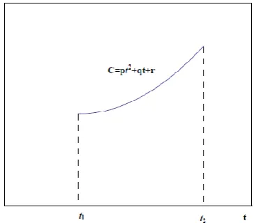
geometry of the input boundary condition is shown in Figure (a).

Fig. (a). Geometry of the input boundary condition

Freeze and Cherry (1979) proposed that dispersion is directly proportional to nth power of the seepage velocity where nth power varies from 1 to 2. In the present case, dispersion due to heterogeneity is considered directly proportional to the square of seepage velocity where as seepage velocity is considered as a linear function of space variable.



ax



u

u 0 1 and





2 0

2

1 ax D D u

D    (5)

where D0 and u0 are initial dispersion

coefficient and seepage velocity respectively.

] [L-1

Substituting values from Eq.(5) in Eq.(1), we have









      _{ }         C x a u x C x a D x t C 1

1 2 ₀

0 (6)

Eqs.(2-4) may be written as:

0 , 0 ; ) ,

(xt C t x

C i (7)







 



2

0 0 0 0

1 2 0 0

                C

D u C u C pt qt r

x

u t t u t t ; x ,t

(8)       x t x t x C , 0 ; 0 ) , ( (9)

Let us introduce a new independent space variable X by a transformation (Kumar et al., (2010)) defined as:







ax



dx dX a x a log X      1 1 1 (10)

Applying the transformation of Eq. (10) on Eqs. (6-9), we have

C X C U X C D t C 0 0 2 2

0 _ 

       (11)

where U₀



u₀aD₀



and 0au0.

0 , 0 ; ) ,

(X t C t X

C i (12)







 



2

0 0 0 0

1 2 0 0

                C

D u C u C pt qt r

X

u t t u t t ; X ,t

(13)       X t X t X C , 0 ; 0 ) , ( (14)

Applying the Laplace transformation on above initial and boundary value problem, it reduces into an ordinary differential equation of second order, which comprises of following three equations:



s



C Ci dX C d U dX C d

D  ₀   ₀ 

2 2

0  (15)

where 



 

0 C(X,t)e dt

C st







 

 











exp



 

2

 

exp



2 exp





; 0

exp 2 exp 2 exp 3 2 2 2 2 2 2 2 2 3 1 2 1 1 1 1 2 1 0 0 0 0                          X s t s p s t s q pt s t s r qt pt s t s p s t s q pt s t s r qt pt C u C u dX C d D (16)    X dX C d ; 0 (17)

where s _{is a Laplace parameter.}

Thus the general solution of ordinary differential equation (15) may be written as:













_

_

1 2 0         i

C X ,s c exp X s

C

c exp X s

s        (18) where 0 0 0 0 0 2 0 2 0 2 1 4 D X U , D , D D U         . Now, using boundary conditions Eq. (16) and (17) in general solution Eq. (18) to eliminate arbitrary constants c1 and c2,

we get the particular solution to the above boundary value problem as:

   

















  

  

 







_{ }

_{ }













s





s



s X C u s t s p s t s q pt s t s r qt pt s t s p s t s q pt s t s r qt pt s s s X C u s C s X

C i i

                                                      0 0 0 3 2 2 2 2 2 2 2 2 3 1 2 1 1 1 1 2 1 0 0 0 exp exp 2 exp 2 exp exp 2 exp 2 exp exp , (19)

Apply Inverse Laplace transformation on Eq.(19) and using the result given by Van

750 back transformations Eq.(10)., the analytical solutions of advection-dispersion equation

for varying type input point source may be written in terms of C x,t as:

 x,t Cexp 0t u0C F X,t ; 0 t t1

C  _i   _i   ₍₂₀₎

   







 1  1   1  1 1 2

1 2 1 0 0 0 0 0 0 ; , 2 , 2 , 2 exp ) , ( exp , t t t t t X J p t t X H q pt t t X G r qt pt D X U C u t X F C u t C t x

C _{i i}

                       (21)    







       





 2  2   2  2 2

2 2 2 1 1 1 1 1 2 1 0 0 0 0 0 0 2 2 2 2 2 t t ; t t , X J p t t , X H q pt t t , X G r qt pt t t , X J p t t , X H q pt t t , X G r qt pt D X U exp C u ) t , X ( F C u t exp C t , x

C i i

                               (22) where

 



_

_





_

_



_

 

_

_       _           _            _     t t X erfc X t t X erfc t X t t X erfc t X t X F                      2 2 exp 2 2 2 exp 2 2 2 exp , 2 0 0 ,

 





 

_       _       _{ }          _              t t X erfc X t X t t X erfc X t X t t t X G                   2 2 exp 4 2 1 4 1 2 2 exp 4 1 4 4 exp . , 2 2 2 ,

 









 

_       _                     _                   _           t t X erfc X t t X t t X erfc X t X t X t t t X t t X H                                 2 2 exp 4 2 2 1 16 2 2 exp 4 2 1 16 4 4 exp 2 1 4 , 2 2 2 2 2 ,

 

 

 





 





 





 

_{ }

 

_{ }

 

X _J

_{ }

_{X t}

t X J X t X J X X t X J X t X J X t X J t X J X t X J , 8 exp , 16 exp , 4 exp exp , 16 2 1 , 4 exp , 2 1 , 4 1 , 7 6 5 4 3 2 1                                  ,  





 





  

            _           _           _    t t X erfc X exp X t t X erfc X exp X t X t exp t t , X J                    2 2 1 2 2 1 4 4

4 2 2 2

 



  





_       _          _                  _                         _        _{ }  t t X erfc t t t X erfc X X t t X erfc X X t X t t X t t X J                            2 2 2 2 2 2 4 3 16 1 2 2 2 exp 2 3 16 1 2 2 1 exp 2 3 4 , 2 2 2 2 2 3 ,  





_       _          _                            _   t t X erfc X t t X erfc X t t X t t t X J                   2 2 2 exp 4 2 2 4 2 2 2 1 exp , 2 4 ,

 







 







_       _                  _                  _                  _      t t X erfc X X t t X erfc X X t t X erfc t t X t t X t t X J                            2 2 3 2 4 4 2 2 2 exp 2 3 4 2 2 2 2 2 1 exp 2 3 4 1 , 2 2 2 2 2 5 ,

 









_       _           _                   _           _  t t X erfc X t t X erfc X t X t t t t X erfc t t X J                     2 2 1 2 4 2 2 2 exp 4 2 2 1 exp 2 2 , 2 6 ,

 

























_       _            _             _                    _         t t X erfc X X t t X erfc X X X t t X erfc t X t X t t X t X t t X X t t X J                                    2 2 9 15 2 2 2 2 exp 12 21 15 12 2 2 4 6 3 3 2 2 1 exp 2 5 2 4 6 15 3 1 , 3 2 2 3 2 2 2 2 2 2 2 2 2 2 7 ,



0



2 _{ }

   ,





a x a log

X  1 ,U0u0aD0,0au0.

RESULTS AND DISCUSSIONS

The analytical solutions obtained as in Eq. (20), Eq.(21) and Eq. (22) are demonstrated with the help of input data to understand the solute concentration distribution behaviour in a finite domain



meter



15 x

0  . The chosen sets of data are taken from the experimental and theoretical published literatures (Todd, 1980; Jaiswal et.al., 2009; Bharati et al., 2015; Singh et al., 2014). The domain is considered

semi-infinite but the solute concentration increases with position in the time domain

day) 2 (

0tt1 and decreases with position

in the time domain tt1(2day) in a finite domain at different values of time.

751 of parameters such as time, dispersion coefficient and heterogeneous parameter. In this study the input parameters values and the ranges of these parameters in which they are varied taken either from published literature or empirical relationship. The concentration values

0

C /

C are evaluated assuming the reference

concentration as C₀ 1.0 , C_i 0.10 . The

common input values are taken as )

(day 01 .

0 -2



p , q0.02(day-1) , r0.03 ,

day 2

1

t _and t2 5day for all cases. The

medium is supposed heterogeneous. In this study source contamination is considered multiple instead of point source contamination.

Case-I: Figures (1-3) demonstrate the concentration behaviour in the time domain



0tt12day



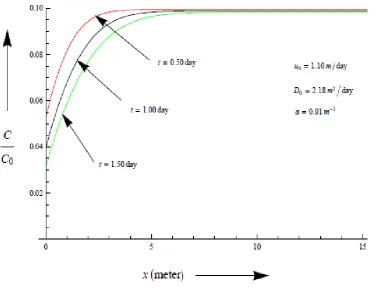
for the analytical solution obtained in Eq. (20).

Figure (1) illustrates the dimensionless concentration profiles at various time

0 . 1 , 5 . 0 (days)

t and 1.5 with common

parameters u₀ 1.10(m/day), D₀2.18(m2/day) , a0.01(m-1). This figure exhibits that the input concentration that is the concentration at the origin of the domain are

054 . 0 , 040 . 0 , 033 .

0 at time t(days)0.5, 1.0

and 1.5, respectively. Concentration level at the source boundary is higher for smaller time and lower for larger time. It attenuates with position and time. It’s also clear that the rate of change in concentration on longitudinal direction is higher for lower time and attains a stationary position after a certain distance travelled onwards.

Fig. 2. Dimensionless concentration distribution evaluated by analytical solution presented in Eq. (20) at various dispersion parameter and velocity for 0tt₁.

The contaminant concentration profile computed with various dispersion coefficient and corresponding seepage velocity D₀ 1.30(m2/day), u₀0.85(m/day) ,

/day) (m 18 .

2 2

0 

D , u₀1.10(m/day) , and /day)

(m 28 .

3 2

0 

D , u₀ 1.35(m/day) with common parameters t1.0(day) and

) (m 01 0. -1

a along longitudinal direction is shown in Figure (2). It is observed from

that the input contaminant concentration on source boundary x0 is 0.040 for different dispersion coefficients. It attenuates with position and time. Enhance in the dispersion of the effluent would cause to its attenuation in the geological formation. The concentration pattern decreases to time, whereas increases to space and after a certain distance travelled it attains a stationary position.

753

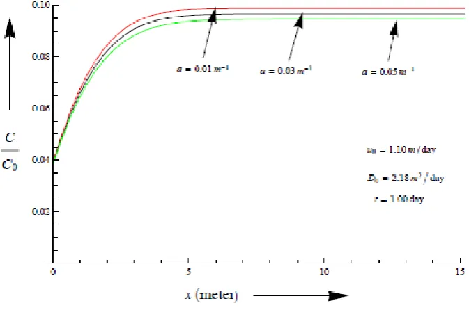
Figure (3) demonstrate the

dimensionless concentration distribution pattern computed at various heterogeneity parameters a(m-1)0.01, 0.03, 0.05 with common parameters t1.0(day) ,

/day) (m 18 .

2 2

0 

D and u01.10(m/day) . It attenuates with position and time. At particular position the concentration level is lower for larger heterogeneous parameter and higher for the smaller heterogeneous parameter. The concentration pattern decreases with respect to heterogeneous parameter, whereas it increases with respect to the space and after a certain distance travelled it becomes constant for all time and space.

Case-II: Figures (4-6) demonstrate the concentration behaviour in the time domain

) day 5 ( )

day 2

( ₂

1 t t

t   for the analytical

solution obtained in Eq. (21).

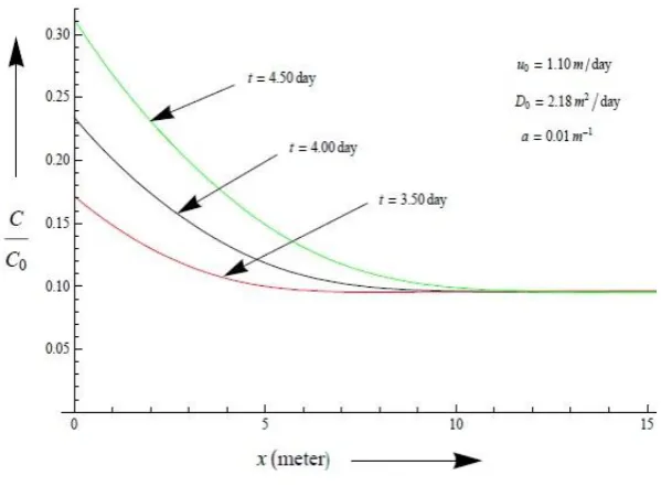
Figure (4) illustrated the dimensionless concentration distribution predicted by the present solution in Eq.(21) with different time t(days)3.5,4.0 and 4.5 computed for the common parameter u₀1.10(m/day) ,

/day) (m 18 .

2 2

0 

D and a0.01(m-1) . The

input concentration C/C0 at the origin (x0)

are respectively 0.170, 0.235, 0.310 at the time t(days)3.5,4.0 and 4.5 , respectively. It attenuates with position and time. At particular position the concentration level is lower for smaller time and higher for larger time. The concentration pattern decreases with respect to space and after a certain distance travelled it becomes constant for all time and space.

Figure (5) represents the dimensionless concentration distribution predicted by the present solution in Eq.(21) at various dispersion parameter and corresponding seepage velocity D01.30(m2/day) ,

(m/day) 85 0

0 .

u  , D0 2.18(m2/day) , (m/day)

10 1

0 .

u  , and D0 3.28(m2/day) , (m/day)

35 1

0 .

u  computed for the common

parameter t4.0(day) , a0.01(m-1) . It attenuates with position and time. At particular position the concentration level is lower for smaller dispersion parameter and higher for larger dispersion parameter. The concentration pattern decreases with respect to space and after a certain distance travelled it becomes constant for all time and space.

Fig. 5. Dimensionless concentration distribution evaluated by analytical solution presented in Eq. (21) at various dispersion parameter and velocity for t₁t t₂.

Fig. 6. Dimensionless concentration distribution evaluated by analytical solution presented in Eq. (21) for various heterogeneous parameter for t₁ t  t₂.

Figure (6) demonstrate the

dimensionless concentration distribution pattern predicted by the present solution in Eq.(21) at various heterogeneous

parameter a(m-1)0.01, 0.03, 0.05, computed for the common parameter t4.0(day) ,

/day) (m 18

2 2

0 .

D  , u01.10(m/day) . It attenuates with position and time. At particular position the concentration level is lower for higher heterogeneous

parameter and higher for the lower

heterogeneous parameter. The

concentration pattern decreases with respect to heterogeneous parameter and space but after certain distance travelled it becomes constant.

755

Fig. 7. Dimensionless concentration distribution evaluated by analytical solution presented in Eq. (22) at various time for tt₂.

Figure (7) illustrated the dimensionless concentration distribution described by the analytical solution in Eq.(22) at different time t(days)6.5,7.0 and 7.5computed for the common parameter u01.10(m/day) ,

/day) (m 18 .

2 2

0 

D , a0.01(m-1) . It attenuates with position and time. At particular position the concentration level

is lower for smaller time and higher for larger time. The input concentration, C/C0

at the origin (x0) are different at each time. The concentration pattern increases with respect to time and decreases with respect to space and after a certain distance travelled it becomes constant for all time and space.

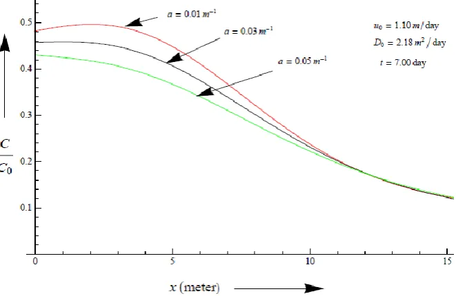
Fig. 9. Dimensionless concentration distribution evaluated by analytical solution presented in Eq. (22) for various heterogeneous parameter for tt₂.

Figure (8) illustrates the solute transport from the point source along the longitudinal direction of the medium, presented in Eq.(22) at various dispersion coefficient and seepage velocity

/day) (m 30

1 2

0 .

D  , u00.85(m/day) ,

/day) (m 18

2 2

0 .

D  , u₀1.10(m/day) and /day)

(m 28

3 2

0 .

D  , u₀1.35(m/day) at time

(day) 0 7.

t and a0.01(m-1). It attenuates with position and time. At particular position the concentration level is lower for smaller dispersion parameter and higher for a larger dispersion parameter. The concentration pattern decreases with space and after a certain distance it attains a stationary position.

Figure (9) illustrates the solute transport described by the solution in Eq.(22), in the time domain tt₂ at various heterogeneity parameters a(m-1)0.01, 0.03, and 0.05 ,

computed at t7.0(day), D₀ 2.18(m2/day), (m/day)

10 . 1

0

u . It attenuates with position and time. At particular position the concentration level is lower for larger heterogeneous parameter and higher for the smaller heterogeneous parameter. The

concentration pattern decreases with respect to heterogeneous parameter and space, but after a certain distance travelled it becomes constant.

CONCLUSIONS

757 dispersion problem. Derived solution can be extended for any time-dependent boundary conditions. The analytical model presented here provides better information about various physical transport parameters.

ACKNOWLEDGEMENT

This research did not receive any specific grant from funding agencies in the public, commercial, or not-for-profit sectors.

REFERENCES

Abramowitz, M. and Stegun, I. A. (1970). Handbook of mathematical functions. First Edition, Dover Publications Inc., New York, 1019.

Aral, M. M. and Liao, B. (1996). Analytical solutions for two-dimensional transport equation with time-dependent dispersion coefficients. J. of Hydrol. Eng., 1(1); 20-32.

Bear, J. (1972). Dynamics of fluids in porous media. New York: Amr. Elsev. Co.

Bharati, V. K., Sanskrityayn, A. and Kumar, N. (2015). Analytical solution of ADE with linear spatial dependence of dispersion coefficient and velocity using GITT. J. of Groundwater Res., 3(4); 13-26.

Chen, J. S., Ni, C. F., Liang, C. P. and Chiang, C. C. (2008). Analytical power series solution for contaminant transport with hyperbolic asymptotic distance-dependent dispersivity. J. of Hydrology, 362(1-2); 142-149.

Chen, J. S., Liu, C. W. and Liao, C. M. (2003). Two-dimensional Laplace-transformed power series solution for solute transport in a radially convergent flow field. Advances in Water Resources, 26; 1113-1124.

Das, P., Begam, S. and Singh, M. K. (2017). Mathematical modeling of groundwater contamination with varying velocity field. J. of Hydrology and Hydromechanics, 65 (2); 192-204.

DeSmedt, F. and Wierenga, P. J. (1978). Solute transport through soil with non-uniform water content. Soil Sci. Soc. Am. J., 42(1); 7-10.

Elfeki, A. M. M., Uffink, G. and Lebreton, S. (2011). Influence of temporal fluctuations and spatial heterogeneity on pollution transport in porous media. Hydrogeology Journal, 20; 283-297.

Flury, M., Wu, Q. J., Wu, L. and Xu, L. (1998). Analytical solution for solute transport with

depth-dependent transformation or sorption coefficient. Water Resour. Res., 34(11); 2931-2937.

Freeze, R. A. and Cherry, J. A. (1979). Groundwater. Prentice-Hall, New Jersey.

Guerrero, J. S. P., Pimentel, L. C. G., Skaggs, T. H. and Van Genuchten, M.Th., (2009). Analytical solution of the advection-diffusion transport equation using a change-of- variable and integral transform technique. Int. J. of Heat and Mass Transfer, 52; 3297-3304.

Harleman, D. R. F. and Rumer, R. R. (1963). Longitudinal and lateral dispersion in an isotropic porous medium. J. of Fluid Mechanics, 16(3); 385-394.

Huang, K., Van Genuchten, M. Th. and Zhang, R. (1996). Exact solutions for one dimensional transport with asymptotic scale-dependent dispersion. Applied Mathematical Modeling, 20; 298-308.

Jaiswal, D. K., Kumar, A., Kumar, N. and Yadav, R. R., (2009). Analytical solutions for temporally and spatially dependent solute dispersion of pulse type input concentration in one-dimensional semi-infinite media. J. of Hydro-environment Research, 2; 254-263.

Kumar, A. and Yadav, R. R. (2015). One-dimensional solute transport for uniform and varying pulse type input point source through heterogeneous medium. Environmental Technology, 36(4); 487-495.

Kumar, A., Jaiswal, D. K. and Kumar, N. (2010). Analytical solutions to one-dimensional advection-diffusion equation with variable coefficients in semi-infinite media. J. of Hydrology, 380; 330-337.

Massabo, M., Cianci, R. and Paladino, O. (2006). Some analytical solutions for two- dimensional Convection-dispersion equation in cylindrical geometry. Environmental Modelling and Software, 21; 681-688.

Moghaddam, M. B., Mazaheri, M. and Vali Samani, J. M. (2017). A comprehensive onedimensional numerical model for solute transport in rivers, Hydrol. Earth Syst. Sci, 21; 99-116.

Ogata, A. and Bank, R. B. (1961). A solution of differential equation of longitudinal dispersion in porous media. U. S. Geol. Surv. Prof. Pap. 411, A1-A7.

Pollution is licensed under a" Creative Commons Attribution 4.0 International (CC-BY 4.0)" Pickens, J. F. and Grisak, G. E. (1981).

Scale-dependent dispersion in a stratified granular aquifer. Water Resources Res., 17(4); 1191-1211.

Rumer, R. R. (1962). Longitudinal dispersion in steady and unsteady flow. J. of Hydraulic Division, 88; 147-173.

Sanskrityayn, A., Bharati, V. K. and Kumar, N. (2016). Analytical solution of ADE with spatiotemporal dependence of dispersion coefficient and velocity using green’s function method, Journal of Groundwater Research, 5(1); 24-31.

Sauty, J. P. (1980). An analysis of hydro-dispersive transfer in aquifers. Water Resources Research, 16(1); 145-158.

Singh, M. K., Ahamad, S. and Singh, V. P., (2014). One-dimensional uniform and time varying solute dispersion along transient groundwater flow in a semi-infinite aquifer. Acta geophysica, 62 (4); 872-892.

Singh, M. K., Kumari, P. and Mahato, N. K. (2013). Two-dimensional solute transport in finite homogeneous porous formations. Int. J. of Geology, Earth & Environmental Sciences, 3(2); 35-48.

Sudicky, E.A. and Cherry, J.A. (1979). Field observations of tracer dispersion under natural flow

conditions in an unconfined sandy aquifer. Fourteenth Canadian Symposium on Water Pollution Research, University of Toronto, Feb. 22, Water Pollution Research, Canada, 14, 1-17.

Todd, D. K., (1980). Groundwater Hydrology. 2nd edn., John Wiley & Sons.

Van Genuchten, M. Th. and Alves, W. J. (1982). Analytical solutions of the one-dimensional convective-dispersive solute transport equation. Technical Bulletin No 1661, US Department of Agriculture.

Volocchi, A. J. (1989). Spatial movement analysis of the transport of kinetically adsorbing solute through stratified aquifers. Water Resources Res., 25; 273-279.

Wierenga, P. J. (1977). Solute distribution profiles computed with steady state and transient. Water Movement Models. Soil Sci. Soc. Amer. J., 41; 1050-1055.