The Short and Long Run Causality between Agglomeration and Productivity

(1)

The Short and Long Run Causality between

Agglomeration and Productivity

Zahra Dehghan Shabani1, Rouhollah Shahnazi2*

Received: December 3, 2016 Accepted: September 28, 2016

Abstract

his study is to investigate the short- and long-run causal relationship between agglomeration (localization and urbanization) economies and labor productivity in the manufacturing sector of 28 Iranian provinces over an 11-year period, 2001–2011. Fully Modified Ordinary Least Squares (FMOLS) method was used to estimate our long-run panel data model. The empirical findings suggested that localization and urbanization economies had a positive and statistically significant effect on labor productivity in the long-run equilibrium. Then, the Generalized Method of Moments (GMM) was employed to examine Granger Causality between each pair of variables. The results revealed a bidirectional short-run Granger causality between localization economies and labor productivity. Additionally, a bidirectional short-run causal relationship was found between urbanization economies and labor productivity for all the manufacturing industries. In the long run, however, there seemed to be bidirectional causality between localization economies and productivity and also between urbanization economies and labor productivity in each manufacturing industry.

Keywords: Agglomeration Economies, Labor Productivity, Granger Causality, Cross-Section Dependence, Iranian Manufacturing Industries.

JEL Classification: C23, R12, L61, L62, L63, L64, L65, L66, L76, L68, L69.

1.Introduction

Agglomeration economies are the benefits that come when firms locate near one another together in cities and industrial clusters. They can be categorized into localization and urbanization economies.

1. Department of Economics, Shiraz University, Shiraz, Iran ([email protected]). 2. Department of Economics, Shiraz University, Shiraz, Iran (Corresponding Author: [email protected]).

(2)

Localization economies exist when the average costs of firms' production in a particular industry shift down due to the expansion in size of the industry. Urbanization economies occur when costs of firms go down because they produce in a densely populated area. So, expansion in an urban area involves benefits to firms from a variety of industries.

Marshall (1920) has proposed three sources of agglomeration economies, namely input sharing, labor market pooling, and knowledge spillovers. Labor market pooling occurs when workers can easily move between firms in an industry. It leads to better skill ‘matches’ between workers and employers. Input sharing includes scale economies in input production that enable firms with greater purchased input intensity will benefit more from being located near the input suppliers.

Knowledge spillovers entail interactions among entrepreneurs and workers in close proximity. It is proportional to the number of firms and while each firm engages in some type of knowledge creation, all the nearby firms can benefit from its outcome (Hu et al., 2015).

The localization economies indicate that productivity is affected by firm clustering productivity. There are some channels through which localization economies affect productivity. First, proximity of the same firms may increase the quantity or improve the quality of the labor pool so that hiring can be done with more exact matches or lower risk and reduce frictional unemployment. Proximity of suppliers can also lead to easier access to or lower costs of material inputs. Second, geographical concentration of firms makes knowledge and skill sharing through formal and informal interactions among firms or individuals possible. The shared knowledge may not be confined to advanced technologies but can also include management skills and business knowledge (Hu et al., 2015). Third, concentration of an industry enables production of specialized intermediate inputs to the optimal level for exploiting scale economies which, in turn, allows firms to outsource higher shares of their intermediate inputs and to specialize in the most profitable activities (Holmes, 1999).

(3)

traffic, causes pollution, and increases the probability of losing some key workers due to the sever competition between plants which, in turn will have a negative impact on productivity.

There are some channels through which urbanization economies influence productivity. Larger cities facilitate spillovers and learning within and across industries. They permit greater specialization and admit more complementarities in production and facilitate sharing and risk-pooling by their very size. Smaller firms in large cities can have access to specialized services offered in large urban areas. Proximity of population concentrations can facilitate product distribution. Moreover, the provision of public goods, due to the consumption of infrastructures which are spread over a large number of people in any one place, can help in achieving significant economies of scale. Finally, home-market effect persuades firms to be located near a large market.

On the other hand, a high degree of urbanization has such disadvantage as congestion, heightened competition, rising land price, intense competition in output markets, and increased trading cost which can negatively impact the productivity of firms located in spatially concentrated regions.

As it was mentioned above, the mainstream regional and urban economic theory supports a causal relationship running from agglomeration to increasing productive efficiency. As a result, much of the empirical research has also assumed the same unidirectionality. More recently, however, a number of researchers have conceded the possibility that density can be determined simultaneously with productivity. They argue that if mobile factors move to the most productive locations, high productivity will give rise to higher densities. This can imply that agglomeration variables are endogenous (Graham et al., 2010).Therefore, some researchers have attempted to correct for potential endogeneity concern, induced through reverse causation, but theoretical and empirical bases for this concern are still largely unknown.

Concerning all the above, this study is aimed at investigating the short- and long-run causality between agglomeration (localization and urbanization) and Productivity in some Iranian Industries.

(4)

Section 4 describes the model we use to test for the directionality of localization and urbanization economies and discusses some estimation issues. Results are presented in Section 5.Conclusions are then drawn in the final section.

2. Literature Review

(5)

(2010) examined the effects of localization, urbanization, and local competition on labor productivity through the use of establishment-level data related to the Korean manufacturing industries. Based on their findings, when an establishment was located in a more localized/specialized, more urbanized/diversified, and more competitive area, the workers, due to the external benefits from agglomeration, became more productive. Martin, Mayer, & Mayneris (2011) assessed the effect of spatial agglomeration of activities on plant-level productivity. To conduct their study, they used French firm and plant-level data from 1996 to 2004. They exploited short-run variations of variables by making use of GMM estimation which allowed them to control for endogeneity biases that appears in the estimation of agglomeration economies. The results showed that French plants benefited from localization economies; however, they found very little evidence for urbanization economies. Dehghan Shabani (2013) investigated the influence of density of economic activity, which is defined as the intensity of labor and physical capital per square kilometer, on labor productivity in 28 Iranian provinces. The empirical results indicated that a high density of economic activity led to an increase in labor productivity in the provinces over the period from 2001 to 2011. Hu, Xu and Yashiro (2015) used the dataset of manufacturing firms active in 176 three-digit industries and in 2860 counties in order to evaluate the role of industrial agglomeration in productivity growth of China's industrial sector. They found that congestion and fiercer competition offset the advantages of agglomeration for firms which were operating within agglomerated regions. They further stated that industrial agglomeration had contributed up to 14% to productivity growth in China's industrial sector between 2000 and 2007. In another study, Azari, Kim, Kim & Ryu (2016) investigated the effect of agglomeration on urban labor productivity in the manufacturing sector of Korea. The researchers benefitted from a panel data analysis of 200 Korean cities during 2004 to 2008. Based on their results, labor density had a negative impact on urban labor productivity, while output density had a positive impact on urban manufacturing productivity.

(6)

research on the impact of productivity on agglomeration. A few researchers, such as Brulhart & Mathys (2008), Ciccone (2002), Ciccone & Hall (1996), Combes et al. (2008), Henderson (1986), and Henderson (2003) have also done some attempts to address the issue of endogeneity in the estimation of agglomeration economies.

Specifically, Graham et al. (2010) examined the long-run causality between productivity and agglomeration (localization and urbanization) economies for different sectors of the UK. The results showed that agglomeration economies were not strictly unidirectional and that higher levels of productivity could induce industrial growth in local and urban environments.

This study contributes to the previous literature through considering both the short- and long- run causality between agglomeration and labor productivity in the Iranian manufacturing industries.

3. Data and Measurement of Agglomeration

Concerning the measurement of industrial agglomeration, The present researchers followed Lall et al. (2004) and used Location quotient (LQ) index for measuring spatial industry concentration (Localization economies). The Location quotient implies the percentage (share) of productive activity of industry i in region j relative to the percentage (share) of total productive activity in region j, expressed in terms of employment. Therefore, * * * * * X X X X S S LQ j i ij j ij C C

ij   (1)

And * 1 i ij n j ij ij ij C X X X X

S  



 and * * * 1 1 1 * X X X X

S _I j

i j j ij I i ij

j  





 

 , j1,...,J ;i1,...,I (2)

(7)

concentration of industry i in region j as compared to the all regions (Nakamura & Paul, 2009).

Although the expressions "population" or "population density", which has often been used as an index for estimating the degree of urbanization in studies that address urbanization economies, might be considered as useful indicators, they are in fact catch-all terms. Especially, such measures are not very adequate for capturing or distinguishing backward linkage effects, such as home market effects where concentration of employment from density of economic activity attracts more firms. Considering this, the present researchers followed Martin et al. (2011) and used two variables to capture urbanization economies. The first one was the number of workers in all industries on region j where industry i was located and the second was the number of workers in industry i and region j. Therefore,

𝐿𝑈𝑡 = ln(𝑒𝑚𝑝𝑙𝑜𝑦𝑒𝑒𝑠𝑡

𝑗

− 𝑒𝑚𝑝𝑙𝑜𝑦𝑒𝑒𝑠_𝑡𝑖𝑗+ 1) (3)

In order to compute LQ and LU, industrial manufacturing employment statistics were collected from statistical yearbook of Iranian provinces provided by the Statistical Center of Iran.

Labor productivity measures the real gross domestic product produced by a labor

L Y

.Value-added and labor force of Iranian Manufacturing Industries were also collected from statistical yearbook of 28 Iranian provinces from 2001 to 2011. The annual data was provided by the Statistical Center of Iran the manufacturing industries were subsumed under International Standard Industrial Classification (ISIC).

4. Econometric Methodology and Results

In this section, the results of short- and Long-run causality between agglomeration and productivity in Iranian Provinces from 2001 to 2011 will be presented. In line with this, the results of cross-section dependence test will be reported first.

4.1. Cross Section Dependence Test

(8)

examine the cross-section of the variables under consideration. It is well known that when T>N (as is the case in this paper). The null hypothesis of Pesaran test is cross-section independence. As Table 1 indicates, however, the null hypothesis of cross-section independence has been rejected. This finding is especially important when one selects unit root and cointegration tests.

Table 1: The Results of Pesaran's Test of Cross Sectional Independence

LU LOC Prob statistic Prob statistic Industry number 0.000 16.15 0.000 17.57

Manufacture of beverages, food and tobacco products 1 0.000 9.58 0.000 9.84

Manufacture of textiles, wearing apparel and leather and related products 2

0.000 3.045 0.000 8.989

Manufacture of wood and of products of wood and cork and furniture 3

0.000 4.21

0.000 11.53

Manufacture of paper and paper products, printing and reproduction of recorded

media 4 0.000 10.37 0.000 31.02

Manufacture of chemical1 5

0.000 7.98

0.000 16.54

Manufacture of other non-metallic mineral products 6 0.000 19.50 0.000 27.37

Manufacture of metals 7

0.000 12.72 0.000 20.48

Manufacture of machinery and equipment and metal products2

8 0.000 4.05 0.000 17.79 Other manufacturing 9 Notes:

1) Authors’ calculations are based on data files obtained from Statistical Center of Iran.

2) The null hypothesis is cross- section independence.

3) LLOC and LU are logarithm Localization and Urbanization economies, respectively.

4.2. Panel Unit Root Tests

This part presents the stationarity properties of the variables under investigation. Although different panel unit root tests, (such as

1. Coke and refined petroleum products, Manufacture of chemicals and chemical products, Manufacture of rubber and plastics products.

(9)

Breitung, 2000; Choi, 2001; Hadri, 2000; Im et al., 2003, Levin et al., 2002; Maddala & Wu, 1999; and Pesaran, 2007) have been mentioned in the literature, and Pesaran's test or CIPS1 test was used in this study because the series were cross-sectionally dependent. Pesaran's test eliminates the probability of cross section dependence by augmenting the ADF regressions with cross section averages. CIPS test assumes that cross-section dependence is in the form of a single unobserved common factor. Regarding Pesaran's (2007) panel unit root test, the following equation has been proposed:

it t i t i it i i

it a b y c y d y e

y      

 _₁ _₁ (4)

Where



 

  

N

i it

t N y

y

1 1 1

1 and





 _



 N

i it

t N y

y

1 1

Then,

The test obtained as



 

 N

i

i N T t N CIPS

1 1

) , (

Where t_i(N,T) is the crosssectionally augmented Dicky-Fuller for the t_ithcross section unit given by the ratio of the coefficient of yit₁

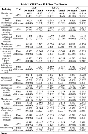
in the regression has been defined by equation 4 (Pesaran, 2007). The results of CIPS test has been provided in Table 2. Based on the obtained findings, the null hypothesis of non-stationarity is accepted. In general, the findings provided evidence that the variables contained a panel unit root. The first differences of these variables were stationary. This meant that the variables were integrated of order one, i.e. I(1).

Given that the variables were integrated of the same order, it was natural for the researchers to proceed with the cointegration test to discover if there was any long-run equilibrium relationship among the variables. This will be focused on in the next section.

(10)

Table 2: CIPS Panel Unit Root Test Results

Industry Test LLP LLOC LU

No trend Trend No trend Trend No trend Trend

Manufacture of beverages, food and tobacco products

Level -0.84 (0.19) -1.57 (0.057) -0.15 (0.439) 0.48 (0.68) -1.249 (0.106) -1.119 (0.132) First difference -6.33 (0.000) -4.39 (0.000) -5.343 (0.000) -2.878 (0.002) -5.666 (0.000) -3.190 (0.001) Manufacture of textiles, wearing apparel and leather and related products

Level 0.199 (0.57) 0.368 (0.644) -0.186 (0.42) -1.721 (0.043) -1.650 (0.059) -1.134 (0.124) First difference -4,00 (0.00) -3.885 (0.000) -7.799 (0.000) -5.282 (0.000) -6.077 (0.000) -3.913 (0.000) Manufacture of wood and of products of

wood and cork and furniture

Level 0.151 (0.560) 0.347 (0.636) -0.594 (0.276) -0.346 (0.365) 0.895 (0.815) -0.174 (0.431) First difference -3.953 (0.000) -2.260 (0.012) -5.950 (0.000) -3.768 (0.000) -4.928 (0.000) -2.723 (0.003) paper and paper products, Printing and reproduction of recorded media

Level -1.825 (0.034) 0.858 (0.805) -1.357 (0.087) -0.533 (0.297) -1.742 (0.041) -0.703 (0.241) First difference -4.91 (0.000) -2.60 (0.004) -5.599 (0.000) -3.039 (0.001) -5.883 (0.000) -4.272 (0.000) Manufacture of chemical

Level 0.614 (0.730) 2.046 (0.980) 0.332 (0.630) 1.811 (0.965) -1.257 (0.112) -1.220 (0.133) First difference -2.709 (0.003) -5.130 (0.000) -3.719 (0.000) -2.889 (0.001) -7.600 (0.000) -5.237 (0.000) Manufacture

of other non-metallic

mineral products

Level _(0.258)-0.646 _(0.981)2.075 _(0.897)1.264 _(0.688)0.490 _(0.233)-0.727 _(0.073)-1.99

First difference -4.359 (0.000) -3.224 (0.001) -5.989 (0.000) -3.575 (0.000) -6.149 (0.000) -3.582 (0.000) Manufacture of basic metals

Level -2.306 (0.011) -0.313 (0.377) -1.459 (0.072) -1.310 (0.095) 0.476 (0.683) -0.365 (0.358) First difference -5.176 (0.000) -2.893 (0.002) -6.613 (0.000) -3.814 (0.000) -5.333 (0.000) -2.843 (0.002) Manufacture of machinery and equipment and metal products

Level -1.050 (0.120) -0.604 (0.273) -1.629 (0.064) -1.424 (0.077) -0.620 (0.268) -1.595 (0.059) First difference -5.618 (0.000) -4.487 (0.000) -5.833 (0.000) -3.200 (0.001) -6.711 (0.000) -3.965 (0.000) Other manufacturing

Level _(0.095)-1.311 _(0.246)-0.687 _(0.091)-1.338 _(0.152)-1.028 _(0.903)1.297 _(0.841)0.998

First difference -3.888 (0.000) -1.770 (0.038) -5.012 (0.000) -1.995 (0.023) -3.363 (0.000) -1.551 (0.081) Notes:

(11)

4.3. Panel Cointegration Tests

To test for cointegration among the variables, the researchers used panel cointegration test proposed by Westerlund (2007) which is indeed derived from the Lagrange multiplier (LM) based unit root tests, such as Ahn (1993), Amsler & Lee (1996), and Schmidt & Phillips (1992) to the test was specifically used to accommodate heteroskedastic and serially correlated errors, individual specific intercepts and time trends, cross-sectional dependence and unknown breaks in both intercepts and slopes of the cointegrated regression. Westerlund (2007) proposed four different statistics to test panel cointegration. Two of them are designed to test the hypothesis that the whole panel is cointegrated, while the other two are group-mean tests. The group mean statistics G_tand G_

test the null hypothesis of no cointegration against the alternative that at least one element in the panel is cointegrated, whereas statistics P_t and

(12)

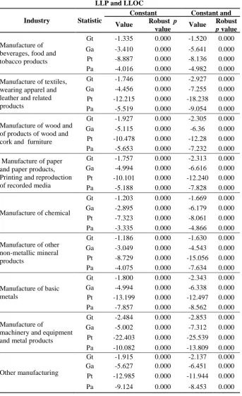
Table 3: The Results of Westerlund Panel Cointegration Test between LLP and LLOC

Industry Statistic

Constant Constant and trend Value Robust p

value Value

Robust

p value

Gt -1.335 0.000 -1.520 0.000

Ga -3.410 0.000 -5.641 0.000

Pt -8.887 0.000 -8.136 0.000

Pa -4.016 0.000 -4.982 0.000

Manufacture of textiles, wearing apparel and leather and related products

Gt -1.746 0.000 -2.927 0.000

Ga -4.456 0.000 -7.255 0.000

Pt -12.215 0.000 -18.238 0.000

Pa -5.519 0.000 -9.054 0.000

Manufacture of wood and of products of wood and cork and furniture

Gt -1.927 0.000 -2.305 0.000

Ga -5.115 0.000 -6.36 0.000

Pt -10.478 0.000 -12.28 0.000

Pa -5.653 0.000 -7.232 0.000

Manufacture of paper and paper products, Printing and reproduction of recorded media

Gt -1.757 0.000 -2.313 0.000

Ga -4.994 0.000 -6.616 0.000

Pt -10.101 0.000 -12.240 0.000

Pa -5.188 0.000 -7.828 0.000

Manufacture of chemical

Gt -1.203 0.000 -1.669 0.000

Ga -2.895 0.000 -6.179 0.000

Pt -7.323 0.000 -8.061 0.000

Pa -3.335 0.000 -4.866 0.000

Manufacture of other non-metallic mineral products

Gt -1.186 0.000 -1.630 0.000

Ga -3.049 0.000 -4.543 0.000

Pt -8.729 0.000 -15.056 0.000

Pa -4.075 0.000 -7.634 0.000

Manufacture of basic metals

Gt -1.800 0.000 -2.343 0.000

Ga -4.994 0.000 -6.338 0.000

Pt -13.199 0.000 -12.497 0.000

Pa -7.857 0.000 -8.562 0.000

Manufacture of

machinery and equipment and metal products

Gt -2.484 0.000 -2.853 0.000

Ga -5.002 0.000 -7.312 0.000

Pt -22.403 0.000 -25.539 0.000

Pa -10.082 0.000 -13.809 0.000

Other manufacturing

Gt -1.915 0.000 -2.137 0.000

Ga -5.627 0.000 -6.451 0.000

Pt -12.985 0.000 -11.944 0.000

(13)

Notes:

1) Authors' calculations are based on data files obtained from Statistical Center of Iran.

2) The null hypothesis is no cointegration.

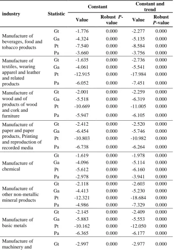
Table 4: The Results of Westerlund Panel Cointegration Test between LLP and LU

industry Statistic

Constant Constant and trend Value Robust P

-value Value

Robust

P-value

Gt -1.776 0.000 -2.277 0.000

Ga -4.324 0.000 -5.135 0.000

Pt -7.540 0.000 -8.584 0.000

Pa -3.660 0.000 -3.756 0.000

Gt -1.635 0.000 -2.736 0.000

Ga -4.061 0.000 -5.541 0.000

Pt -12.915 0.000 -17.984 0.000

Pa -6.052 0.000 -7.451 0.000

Gt -2.001 0.000 -2.259 0.000

Ga -5.518 0.000 -6.319 0.000

Pt -10.669 0.000 -11.005 0.000

Pa -5.947 0.000 -6.105 0.000

Gt -2.412 0.000 -2.520 0.000

Ga -6.454 0.000 -5.746 0.000

Pt -10.803 0.000 -10.982 0.000

Pa -6.738 0.000 -6.264 0.000

Gt -1.619 0.000 -1.978 0.000

Ga -4.096 0.000 -5.114 0.000

Pt -5.612 0.000 -6.160 0.000

Pa -2.978 0.000 -3.941 0.000

Gt -2.118 0.000 -2.603 0.000

Ga -4.413 0.000 -5.230 0.000

Pt -12.321 0.000 -18.684 0.000

Pa -4.986 0.000 -7.329 0.000

Gt -2.145 0.000 -2.409 0.000

Ga -5.883 0.000 -5.553 0.000

Pt -10.162 0.000 -12.050 0.000

Pa -6.365 0.000 -6.177 0.000

Manufacture of

(14)

equipment and metal products

Ga -7.152 0.000 -7.082 0.000

Pt -31.030 0.000 -22.020 0.000

Pa -12.831 0.000 -9.891 0.000

Other

manufacturing

Gt -2.316 0.000 -2.117 0.000

Ga -6.785 0.000 -5.818 0.000

Pt -10.919 0.000 -10.844 0.000

Pa -6.932 0.000 -7.426 0.000

Notes:

1) Authors' calculations are based on data files obtained from Statistical Center of Iran.

2) The null hypothesis is no cointegration.

The results of this test, as depicted in Tables 3 and 4, confirmed the existence of co-movement among the series. Therefore, there is a long-run equilibrium relationship between agglomeration (urbanization and localization) and productivity.

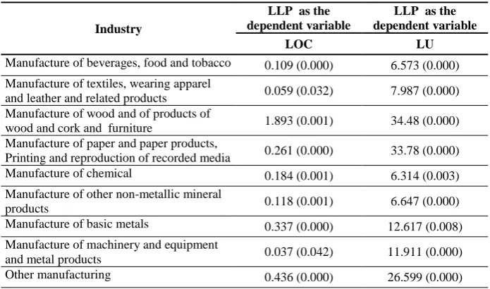
4.5. Panel Long-Run Elasticities

The long-run equilibrium relationship between the agglomeration (urbanization and localization) and productivity was examined through the use of the fully modified OLS (FMOLS) technique. Pedroni (2001) FMOLS is an estimation technique of non-parametric type which is useful for handling with the problems of endogenous regressors and serial correlation in the error term. The technique allows the researchers to have consistent and efficient estimators of the long-run relationship. As Table 5 indicates, all the variables had the expected sign and were statistically significant at a 0.05 level of significance.

(15)

Table 5: The Results of the Fully Modified OLS Estimates Technique (FMOLS)

LLP as the dependent variable LLP as the

dependent variable Industry

LU LOC

6.573 (0.000) 0.109 (0.000)

Manufacture of beverages, food and tobacco

7.987 (0.000) 0.059 (0.032)

34.48 (0.000) 1.893 (0.001)

33.78 (0.000) 0.261 (0.000)

6.314 (0.003) 0.184 (0.001)

6.647 (0.000) 0.118 (0.001)

12.617 (0.008) 0.337 (0.000)

11.911 (0.000) 0.037 (0.042)

Manufacture of machinery and equipment and metal products

26.599 (0.000) 0.436 (0.000)

Other manufacturing

Notes:

1) Authors' estimation is based on data files obtained from Statistical Center of Iran. 2) p values have been provided in parentheses.

4.6 Panel Causality Tests

To test for the presence short- and Long-run causality between agglomeration and productivity, the present researchers drew from the concept of Granger causality and used a panel vector error-correction model (Pesaran et al., 1999) which is a two-step procedure (Engle & Granger, 1987) estimated to perform Granger-causality tests. First, the long-run equilibrium model was estimated in order to obtain the estimated residuals which were then these residuals lagged for one period and used as the error correction term. The equations for Granger-causality test associated with the error correction term have been presented below.

∆LLPit= α1j+ ∑ π11_iq p

q=1 ∆LLPit−q+ ∑ π12_iq∆LUit−q p

q=1 + ξ1iECTit−1+ ω1it (1)

∆LUit= α2j+ ∑ π21_iq p

q=1 ∆LUit−q+ ∑ π22_iq∆LLPit−q p

q=1 + ξ2iECTit−1+ ω2it (2) The equations for Granger-causality between localization (LOC) and Labor productivity (LLP) are:

∆LLPit= α1j+ ∑ π31iq

p

q=1 ∆LLPit−q+ ∑ π32iq∆LOCit−q

p

(16)

∆LOCit= α2j+ ∑ π41iq

p

q=1 ∆LOCit−q+ ∑ π42iq∆LLPit−q

p

q=1 + ξ4iECTit−1+ ω2it(4) In the above equations, p is the lag length set that was selected based on the Schwarz Bayesian information criteria (SBC). ECT

Stands for error correction term (For checking Long-run causality) and ω refers to serially uncorrelated error term.

Two sources of causation can be derived from estimation of the dynamic error correction model, the short- and long-run causality. For instance, if π12iq =0 iqis rejected, then short causality runs from ∆LU to ∆LLP . Similarly, if π₂₂_iq = 0iq is rejected, there will be

short-run causality from ∆LLP to ∆LU . Concerning the long run causality, the present researchers considered the significance of error correction term. For instance, the significance of ξ1i=0 i means that ∆LLP responds to deviations from the long-run equilibrium, whereas the significance of ξ_2i=0 _i implies that ∆𝐿𝑈 responds to deviation from the long-run equilibrium.

(17)

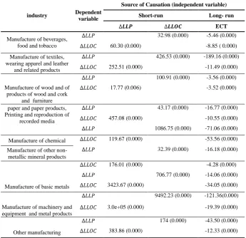
Table 6: The Results of Panel Causality Tests

Source of Causation (independent variable) Dependent

variable

industry Short-run Long- run ECT

∆𝑳𝑳𝑶𝑪 ∆𝑳𝑳𝑷

-5.46 (0.000) 32.98 (0.000)

∆𝐿𝐿𝑃 Manufacture of beverages,

food and tobacco ∆𝐿𝐿𝑂𝐶 60.30 (0.000) -8.85 ( 0.000) -189.16 (0.000) 426.53 (0.000)

∆𝐿𝐿𝑃 Manufacture of textiles,

wearing apparel and leather

and related products ∆𝐿𝐿𝑂𝐶 252.51 (0.000) -11.49 (0.000) -3.56 (0.000) 100.91 (0.000)

∆𝐿𝐿𝑃

-3.52 (0.000) 17.77 (0.006)

∆𝐿𝐿𝑂𝐶 Manufacture of wood and of

products of wood and cork and furniture

-16.77 (0.000) 43.17 (0.000)

∆𝐿𝐿𝑃 paper and paper products,

Printing and reproduction of

recorded media ∆𝐿𝐿𝑂𝐶 457.08 (0.000) -10.55 (0.000) -71.06 (0.000) 1086.75 (0.000)

∆𝐿𝐿𝑃

-53.56 (0.000) 119.67 (0.000)

∆𝐿𝐿𝑂𝐶 Manufacture of chemical

-16.18 (0.000) 32.39 (0.000)

∆𝐿𝐿𝑃 Manufacture of other

non-metallic mineral products

-4.28 (0.000) 176.01 (0.000)

∆𝐿𝐿𝑂𝐶

-14.06 (0.000) 706.77 (0.000)

∆𝐿𝐿𝑃

-34.05 (0.000) 3423.67 (0.000)

∆𝐿𝐿𝑂𝐶 Manufacture of basic metals

-121.36(0.000) 9492.23 (0.000)

∆𝐿𝐿𝑃

-19.39 (0.000) 3.0e+05 (0.000)

∆𝐿𝐿𝑂𝐶 Manufacture of machinery and equipment and metal products

-43.50 (0.000) 174 (0.000)

∆𝐿𝐿𝑃

-12.33 (0.000) 383.86 (0.000)

∆𝐿𝐿𝑂𝐶 Other manufacturing

Notes:

1) Authors' estimation is based on data files obtained from Statistical Center of Iran. 2) Partial F-statistics reported with respect to short-run changes in the independent

variables while t-statistic reported with respect to long-run. 3) p-values are given in parentheses.

With regard to reverse causation, granger causality was running from labor productivity to localization for all the manufacturing industries. This suggests that localization economies are indeed endogenous and the lagged values of productivity help in predicting localization for all manufacturing industries and vice versa. Overall, the results of short-run panel causality test showed a bidirectional granger causality between localization and labor productivity.

Considering the long-run causality, results revealed bidirectional causality between localization and productivity.

(18)

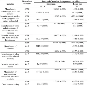
productivity in all the manufacturing industries. This can imply that we can predict productivity level via information about urbanization level.

Table 7: The Results of Panel Causality Tests

Source of Causation (independent variable) Dependent

variable

industry Short-run Long- run ECT ∆𝑳𝑼 ∆𝑳𝑳𝑷 -15.69 (0.000) 265.61 (0.000) ∆𝐿𝐿𝑃 Manufacture

of beverages, food and

tobacco ∆𝐿𝑈 450.77 (0.000) -7.78 (0.000) -126.54 (0.000) 1574.7 (0.000)

∆𝐿𝐿𝑃 Manufacture of textiles,

wearing apparel and leather and related

products -12.86 (0.000) 2137.15 (0.000) ∆𝐿𝑈 -5.32 (0.000) 13.29 (0.009) ∆𝐿𝐿𝑃 -3.61 (0.000) 47.77 (0.000) ∆𝐿𝑈 Manufacture of wood

and of products of wood and cork and

furniture

-25.94 (0.000) 584.55 (0.000)

∆𝐿𝐿𝑃 Manufacture of paper

and paper products, Printing and reproduction of recorded media -17.58 (0.000) 3892.49 (0.000) ∆𝐿𝑈 -769.59 (0.000) 14356.8 (0.000) ∆𝐿𝐿𝑃 -69.30 (0.000) 2712.25 (0.000) ∆𝐿𝑈 Manufacture of chemical -82.23 (0.000) 188.14 (0.000) ∆𝐿𝐿𝑃 -31.72 (0.000) 5352.20 (0.000) ∆𝐿𝑈 Manufacture of other

non-metallic mineral products -50.06 (0.000) 5.35 (0.068) ∆𝐿𝐿𝑃 -4.80 (0.000) 12.29 (0.006) ∆𝐿𝑈 Manufacture of basic

metals -112.01 (0.000) 286.94 (0.000) ∆𝐿𝐿𝑃 -26.57 (0.000) 878.79 (0.000) ∆𝐿𝑈 Manufacture of machinery and equipment and metal

products

-45.32 (0.000) 172.18 (0.000)

∆𝐿𝐿𝑃

-12.02 (0.000) 289.55 (000)

∆𝐿𝑈 Other manufacturing

Notes:

1) Authors' estimation is based on data files obtained from Statistical Center of Iran. 2) Partial F-statistics reported with respect to short-run changes in the independent

variables while t-statistic reported with respect to long-run. 3) p-values are given in the parentheses.

(19)

tobacco, Manufacture of textiles, wearing apparel and leather and related products, Manufacture of wood and of products of wood and cork and furniture , Manufacture of paper and paper products, Printing and reproduction of recorded media, Manufacture of chemical, Manufacture of basic metals, Manufacture of machinery and equipment and metal products, Other manufacturing products.

As predicted by the theory, the results of the present study revealed that both localization and urbanization affected labor productivity for all the manufacturing industries. The results further offered the evidence for endogenous agglomeration economies.

5. Conclusion

(20)

bidirectional causality was found between agglomeration and productivity.

the results of the present study can becomes helpful for policy makers to recognize the new evidence from relationship between productivity and agglomeration, because Agglomeration economies are also important policy issues for regional municipalities, because they engender industrial clustering and clusters bring productivity gains in the short run and long run. Furthermore, policy makers attention to level of productivity because it can induce growth in the scale of local urban and industrial environments.

References

Azari, M., Kim, H., Kim, J. Y., & Ryu, D. (2016). The Effect of Agglomeration on the Productivity of Urban Manufacturing Sectors in a

Leading Emerging Economy. Economic Systems, Retrieved from

http://www.sciencedirect.com/science/article/pii/S0939362516300036/ pdfft ? md5 =5c36c363f9a81c956113f54a281808c2&pid=1-s2.0-S0939362516300036-main.pdf.

Brülhart, M., & Mathys, N. A. (2008). Sectoral Agglomeration Economies in a Panel of European Regions. Regional Science and Urban Economics, 38(4), 348-362.‏

Ciccone, A. (2002). Agglomeration Effects in Europe. European Economic Review, 46(2), 213-227.‏

Ciccone, A., & Hall, R. E. (1996). Productivity and the Density of Economic Activity. The American Economic Review, 86, 54-70. Choi, I. (2001). Unit Root Tests for Panel Data. Journal of International Money and Finance, 20(2), 249-272.

(21)

Combes, P. P., Duranton, G., & Gobillon, L. (2008). Spatial Wage Disparities: Sorting Matters. Journal of Urban Economics, 63(2), 723-742.‏ Graham, D. J., Melo, P. S., Jiwattanakulpaisarn, P., & Noland, R. B. (2010). Testing for Causality between Productivity and Agglomeration Economies. Journal of Regional Science, 50(5), 935-951.‏

Hadri, K. (2000). Testing for Stationarity in Heterogeneous Panel Data. The Econometrics Journal, 3(2), 148-161.‏

Henderson, J. V. (1986). Efficiency of Resource Usage and City Size.

Journal of Urban Economics, 19(1), 47-70.

Henderson, J. V. (2003). Marshall's Scale Economies. Journal of Urban Economics, 53(1), 1-28.

Holmes, T. J. (1999). Localization of Industry and Vertical Disintegration. Review of Economics and Statistics, 81(2), 314-325. Hu, C., Xu, Z., & Yashiro, N. (2015). Agglomeration and Productivity in China: Firm Level Evidence. China Economic Review, 33, 50-66.‏ Im, K. S., Pesaran, M. H., & Shin, Y. (2003). Testing for Unit Roots in Heterogeneous Panels. Journal of Econometrics, 115(1), 53-74.‏ Jacobs, J. (1969). The Economy of Cities. New York: Vintage.

Ke, S. (2010). Agglomeration, Productivity, and Spatial Spillovers across Chinese Cities. The Annals of Regional Science, 45(1), 157-179.

Lall, S. V., Shalizi, Z., & Deichmann, U. (2004). Agglomeration

Economies and Productivity in Indian Industry. Journal of

Development Economics, 73(2), 643-673.‏

Lee, B. S., Jang, S., & Hong, S. H. (2010). Marshall’s Scale Economies and Jacobs’ Externality in Korea: the Role of Age, size and the Legal form of Organization of Establishments. Urban Studies,

(22)

Levin, A., Lin, C. F., & Chu, C. S. J. (2002). Unit Root Tests in Panel

Data: Asymptotic and Finite-Sample Properties. Journal of

Econometrics, 108(1), 1-24.‏

Maddala, G. S., & Wu, S. (1999). A Comparative Study of Unit Root Tests with Panel Data and a New Simple Test. Oxford Bulletin of Economics and Statistics, 61(S1), 631-652.‏

Maré, D. C., Timmons, J., & Economic, M. (2006). Geographic Concentration and Firm Productivity. Motu Working Paper, Retrieved from http://motu-www.motu.org.nz/wpapers/06_08.pdf.

Martin, P., Mayer, T., & Mayneris, F. (2011). Spatial Concentration and Plant-Level Productivity in France. Journal of Urban Economics,

69(2), 182-195.‏

Marshall, A. (1920). Principles of Economics. London: Mac-Millan. Nakamura, R., & Paul, C. J. M. (2009). 16 Measuring Agglomeration.

Retrieved from https://books.google.com.

Pedroni, P. (2004). Panel Cointegration: Asymptotic and Finite Sample Properties of Pooled Time Series Tests with an Application to the PPP Hypothesis. Econometric Theory, 20(03), 597-625.‏

--- (2000). Fully Modified OLS for Heterogeneous Cointegrated Panels. Advanced in Econometrics, 15, 93-130.

Pesaran, M. H. (2007). A Simple Panel Unit Root Test in the Presence of Cross‐Section Dependence. Journal of Applied Econometrics,

22(2), 265-312.‏

--- (2004). General Diagnostic Tests for Cross Section Dependence in Panels. Cambridge Working Papers in Economics,

Retrieved from

(23)

Pesaran, M. H., Shin, Y., & Smith, R. P. (1999). Pooled Mean Group

Estimation of Dynamic Heterogeneous Panels. Journal of the

American Statistical Association, 94(446), 621-634.‏

Rosenthal, S. S., & Strange, W. C. (2004). Evidence on the Nature and Sources of Agglomeration Economies. Handbook of Regional and Urban Economics, 4, 2119-2171.‏

Westerlund, J. (2005). New Simple Tests for Panel Cointegration.