Numerical solution of delay differential equations via operational matrices of hybrid of block-pulse functions and Bernstein polynomials

(1)

Numerical solution of delay diﬀerential equations via opera-tional matrices of hybrid of block-pulse functions and Bernstein polynomials

M. Behroozifar

Faculty of Basic Sciences, Babol University of Technology, Babol, Mazandaran, Iran.

E-mail: m [email protected]

S. A. Yousefi

Department of Mathematics, Shahid Beheshti University, Tehran, Iran.

E-mail: [email protected] Corresponding Author

Abstract _{In this paper, we introduce hybrid of block-pulse functions and Bernstein} polynomials and derive operational matrices of integration, dual, differenti-ation, product and delay of these hybrid functions by a general procedure that can be used for other polynomials or orthogonal functions. Then, we utilize them to solve delay differential equations and time-delay system. The method is based upon expanding various time-varying functions as their trun-cated hybrid functions. Illustrative examples are included to demonstrate the validity, efficiency and applicability of the method.

Keywords. Delay diﬀerential equation, Bernstein polynomial, Hybrid of block-pulse function, Op-erational matrix.

2010 Mathematics Subject Classification. 65L05, 34K06, 34K28.

1. Introduction

Delays occur frequently in biological, chemical, electronic and transporta-tion systems [10]. Time-delay systems are therefore a very important class of systems whose control and optimization have been of interest to many investigators. Orthogonal functions and polynomial series have received con-siderable attention in dealing with various problems of dynamic systems. The main characteristic of this technique is that it reduces these problems to those of solving a system of algebraic equations, thus greatly simplifying the prob-lems [2, 3,7, 9,12,19]. The approach is based on converting the underlying diﬀerential equations into integral equations through integration, approximat-ing various signals involved in the equation by truncated polynomials series and using the operational matrices to eliminate the integral, derivation and delay operations. Special attention has recently been given to applications

(2)

of Walsh function [3], Haar wavelets [6], Chebyshev polynomials [7], Bessel functions [16], Legendre polynomials [2] , Legendre wavelets [17] , Sine-cosine wavelets [18] and Bernstein polynomials [23]. In recent years the diﬀerent kinds of hybrid functions [4, 5, 8, 9, 11, 12, 13, 14, 19, 20] were applied to solve the delay problem.

Bernstein polynomials have some properties that distinguish it from other polynomials for example continuity and partition of unity property. All of the Bernstein polynomials vanish at the initial and end points of the interval [a, b] except for the first polynomial and the last polynomial are equal to 1 at x = a and x = b, respectively, which provides greater flexibility to im-pose boundary conditions. The Bernstein polynomials, although not based on orthogonal polynomials, can also be applied to analyze various problems. Specifically, in [24,25] Bernstein polynomials have been used for solving the partial differential equation.

In this paper, hybrid of block-pulse functions and Bernstein polynomials are introduced and derived operational matrices of integration P, dual Q, differentiation D, product Cb and delay Del by a general procedure. These matrices are applied to evaluate the solution of delay differential equation or delay differential system by expanding the candidate function as hybrid functions with unknown coefficients and reducing the delay problem to a set of algebraic equations.

This paper is organized as follows: In section 2 we describe the basic formu-lation of Bernstein polynomials which is required for our subsequent develop-ment. Section 3 is devoted to the definition of hybrid of block-pulse functions and Bernstein polynomials and function approximation using these functions. In section 4 we calculate the operational matrices of integration, dual, differ-entiation, product and delay. In section 5, we report our numerical findings which demonstrate the validity, accuracy, efficiency and applicability of the operational matrices by considering some test problems. Section 6 consists of a brief summary.

2. Properties of Bernstein polynomials

The Bernstein polynomials of mth-degree are deﬁned on the interval [a, b] as [1]

Bi,m(x) =

(

m i

)

(x−a)i(b−x)m−i

(b−a)m , i= 0,1, . . . , m,

where ₍

m i

)

= m!

(3)

These Bernstein polynomials form a basis onL2[a, b]. There arem+ 1 poly-nomials ofmth-degree. For convenience, we setBi,m(x) = 0, ifi <0 ori > m.

A recursive deﬁnition can also be used to generate the Bernstein polynomials over [a, b] so that the ith Bernstein polynomial ofmth-degree can be written

Bi,m(x) =

(b−x)

b−a Bi,m−1(x) +

(x−a)

b−a Bi−1,m−1(x).

It can readily be shown that each of the Bernstein polynomials is positive and the sum of all the Bernstein polynomials is unity for all real x ∈ [a, b], i.e., ∑m

i=0Bi,m(x) = 1 (unity partition property). It is easy to show that any given

polynomial ofmth-degree can be expanded in terms of these basis functions.

3. Properties of hybrid functions

3.1. Hybrid of block-pulse functions and Bernstein polynomials. Since interval [a, b) can be shifted to [0,1), therefor we concentrate on [0,1). Hybrid of block-pulse functions and Bernstein polynomials are deﬁned on [0,1) for

i= 0,1, . . . , mand n= 0,1, . . . , N−1,

ψi,n(t) =

{

Bi,m(kt−n) n_k ≤t < n+1_k

0 otherwise, (3.1)

where m is the degree of Bernstein polynomial on [0,1], n is transmission parameter, N denotes the number of subinterval of [0,1] and the parameters

k, N will be speciﬁed.

3.2. Function Approximation. Suppose thatH=L2[0,1] and{ψi,n(t)}m,Ni=0,n=0−1 ⊂

H be the set of hybrid functions of Bernstein polynomials of mth-degree and

Y =Span{ψi,n(t) |i= 0,1,· · ·m, n= 0,1,· · · , N−1}

and f be an arbitrary element in H. Since Y is a ﬁnite dimensional vector space,f has the unique best approximation out of Y such asy0 ∈Y, that is

∃y0∈Y; ∀y∈Y ||f −y0||2 ≤ ||f −y||2,

where||f||2₂ =< f, f >=∫₀1f2(x)dx.

Sincey0 ∈Y, there exist the unique coeﬃcientsci,n such that

f ≃y0 = N_∑−1

n=0 m

∑

i=0

ci,nψi,n=cTϕ,

where

ϕT = [ψ0,0 , ψ1,0 ,· · · , ψm−1,0 , ψm,0,· · · , ψ0,N−1, ψ1,N−1 ,· · · , ψm−1,N−1 , ψm,N−1],

(4)

andcT can be obtained by

cT < ϕ , ϕ >=< f, ϕ >,

where

< f, ϕ >= ∫ 1

0

f(x)ϕ(x)Tdx

and< ϕ , ϕ >is aN(m+ 1)×N(m+ 1) matrix which is said dual operational matrix ofϕ and denoted byQ

Q=< ϕ , ϕ >= ∫ 1

0

ϕ(x)ϕ(x)Tdx,

then

cT = (∫ 1

0

f(x)ϕ(x)Tdx

)

( Q )−1. (3.2)

In the following lemma we present an upper bound for the error approximation.

Lemma 3.1. Suppose that the function g: [0,1)→R is m+ 1 times contin-uously diﬀerentiable, g∈Cm+1[t0, tf]

and Y = Span{ψi,n(t) | i = 0,1,· · ·m, n = 0,1,· · · , N −1}. If cTϕ is

the best approximation g out of Y then the mean error bounded is presented as follows:

||g−cTϕ||2≤

M

(m+ 1)! km+1 √₂_m_{+ 3} ,

where M = maxx∈[t0,tf]|g

(m+1)₍_x₎_|_.

Proof. We consider the Taylor polynomial of ordermfor functiongon [n_k,n+1_k )

yn(x) =g(

n k) +g

′₍n

k)(x− n

k) +· · ·+g

(m)₍n

k)

(x−n_k)m

m! forn= 0,1,· · · , N −1 which we know

|g(x)−yn(x)| ≤ |g(m+1)(η)|

(x−n_k)m+1

(m+ 1)! (3.3)

whereη ∈(n_k,n+1_k ).Since cTϕ is the best approximation g out of Y, yn ∈Y

and using (3.3) we have

||g−cTϕ||2₂= ∫ 1

0

|g(x)−cTϕ(x)|2dx=

N_∑−1

n=0

∫ n+1

k

n k

|g(x)−cTϕ(x)|2dx

≤

N_∑−1

n=0

∫ n+1

k

n k

|g(x)−yn(x)|2dx≤ N_∑−1

n=0

∫ n+1

k

n k

[

g(m+1)(η)(x−

n k)m+1

(m+ 1)! ]2

(5)

≤ M2 (m+ 1)! 2

N_∑−1

n=0

∫ n+1

k

n k

(x−n k)

2m+2_dx₌ M2

[(m+ 1)! ]2 _k2m+2 ₍₂_m_{+ 3)},

and by taking square root we have the above bound.

The presented upper bound of the error depends on _(m+1)!_km1+1 √_2m+3 which shows that the error reduces to zero very fast as m increase. This is one of the advantages of hybrid of block-pulse functions and Bernstein poly-nomials.

4. Operational matrices of hybrid of block-pulse functions and Bernstein polynomials

4.1. Operational matrix of integration. The operational matrix of inte-grationP is given by

∫ x

0

ϕ(t)dt≃P ϕ(x), 0≤x <1.

For obtaining an explicit formula forP we denote the vector

B(kx−n) =     

B0,m(kx−n)

B1,m(kx−n)

.. .

Bm,m(kx−n)

    =

    

ψ0,n(x)

ψ1,n(x)

.. .

ψm,n(x)

    

forn= 0,1,· · · , N −1

ϕ(x) =               

B(kx) 0≤x < 1_k

B(kx−1) 1_k ≤x < 2_k B(kx−2) 2_k ≤x < 3_k

.. .

B(kx−(N−1)) N_k−1 ≤x <1 .

, (4.1)

It is easy to see that: ∫ 1

0

(1−x)rxidx= 1

(r+i+ 1)(r+i_i ), i, r ∈N∪ {0}

therefore _∫

1

0

Bi,m(x)dx=

1

(6)

so

∫ 1

0

B(x)dx=      1 m+1 1 m+1 .. . 1 m+1      then ∫ 1 0

B(kx−n)dx=       1 k(m+1) 1 k(m+1) .. . 1 k(m+1)     

, n= 0,1,· · ·, N −1. (4.2)

On the other hand we know ∫ x

0

B(t)dt≃P B(x), 0≤x≤1 (4.3)

which P is the operational matrix of integration of B(x) and the details of obtaining this matrix is given in [23]. Now, we want to obtain the operational matrix of integrationP using (4.2), (4.3) and the property of partition of unity of Bernstein polynomial

∫ x

0

B(kt)dt=                  ∫x

0 B(kt)dt 0≤x <

1 k

∫1

k

0 B(kt)dt+

∫x

1

k B(kt)dt

1

k ≤x < 2 k .. . ∫1 k

0 B(kt)dt+

∫2

k

1

k

B(kt)dt+· · ·+∫Nx−1

k B(kt)dt N−1

k ≤x < N k =                                              P

kB(kx), 0≤x <

1 k       1 k(m+1) 1 k(m+1) .. . 1 k(m+1)      +      0 0 .. . 0    

= k(m+1)1 B(kx−1),

1

k ≤x < 2 k .. .       1 k(m+1) 1 k(m+1) .. . 1 k(m+1)      +      0 0 .. . 0     +. . .+      0 0 .. . 0    

= k(m+1)1 B(kx−(N−1)), N−1

k ≤x < N

(7)

which 1 is a matrix (m+ 1)×(m+ 1) that all of its elements is 1, therefore

∫ x

0

B(kt)dt= [

P k,

1

k(m+ 1),· · · , 1

k(m+ 1) ]     

B(kx)

B(kx−1) .. .

B(kx−(N−1))      = [ P k, 1

k(m+ 1),· · ·, 1

k(m+ 1) ]

ϕ(x).

Similarly, we have

∫x

0

B(kt−1)dt=

                 ∫x

0 B(kt−1)dt 0≤x <

1

k

∫1 k

0 B(kt−1)dt+

∫x

1

kB(kt−1)dt

1

k≤x <

2 k . .. ∫1 k

0 B(kt−1)dt+

∫2 k 1 k

B(kt−1)dt+· · ·+∫Nx−1 k

B(kt−1)dt N−1

k ≤x < N k =                                                                         0 0 .. . 0    

= 0 B(kx) 0≤x < 1k

P

kB(kx−1)

1

k ≤x < 2 k       1 k(m+1) 1 k(m+1) .. . 1 k(m+1)      = 1

k(m+1)B(kx−2)

2

k ≤x < 3 k .. .       1 k(m+1) 1 k(m+1) .. . 1 k(m+1)      = 1

k(m+1)B(kx−(N −1)) N−1

k ≤x < N

k

then ∫ x

0

B(kt−1)dt= [

0,P k,

1

k(m+ 1),· · · , 1

k(m+ 1) ]

ϕ(x)

(8)

obtained as follows

P =

        

P k

1 k(m+1)

1

k(m+1) · · · 1 k(m+1)

0 P_k _k(m+1)1 · · · _k(m+1)1

0 0 P_k · · · _k(m+1)1 ..

. ... ... · · · ...

0 0 0 · · · P_k

        

.

4.2. Dual operational matrix. We deﬁne the dual operational matrix of ϕ

in the preceding section that

Q=

∫ 1

0

ϕ(x)ϕT(x)dx.

In [23] the dual operational matrix ofB(x) is presented

Q=

∫ 1

0

B(x)BT(x)dx.

We have ∫ 1

0

B(kx−n)B(kx−n)Tdx= ∫ n+1

k

n k

B(kx−n)B(kx−n)Tdx= Q

k,

(4.4)

∫ 1

0

B(kx−n)B(kx−j)Tdx= 0 , n̸=j (4.5)

forj, n= 0,1,· · · , N −1. By using (4.4) and (4.5)

Q=

∫ 1

0

ϕ(x)ϕT(x)dx

=

     

∫1

0 B(kx)B(kx)

T_dx _{· · ·} ∫1

0 B(kx)B(kx−(N−1))

T_dx

∫1

0 B(kx−1)B(kx)

T_dx _{· · ·} ∫1

0 B(kx−1)B(kx−(N−1))

T_dx

.

.. · · · ...

∫1

0 B(kx−(N−1))B(kx)

T_dx _{· · ·} ∫1

0 B(kx−(N−1))B(kx−(N−1))

T_dx

     

= 1

k

    

Q 0 · · · 0 0 Q · · · 0

..

. ... · · · ... 0 0 · · · Q

(9)

4.3. Operational matrix of diﬀerentiation. The operational matrix of diﬀerentiationD is given by

dϕ(x)

dx =Dϕ(x).

We have

dB(x)

dx =D B(x) (4.6)

whichDis the operational matrix of diﬀerentiation ofB(x) and the details of obtaining this matrix is given in [23].

The operational matrix of diﬀerentiationDis obtained using (4.6) as follows

d

dxϕ(x) =

                    

d

dxB(kx) 0≤x <

1 k

d

dxB(kx−1)

1

k ≤x < 2 k

d

dxB(kx−2)

2

k ≤x < 3 k

.. .

d

dxB(kx−(N −1)) N−1k ≤x < N

k

=                     

kD B(kx) 0≤x < 1_k

kD B(kx−1) 1_k ≤x < 2_k

kD B(kx−2) 2_k ≤x < 3_k

.. .

kD B(kx−(N−1)) N_k−1 ≤x < N_k

so

D=k

    

D 0 0 · · · 0 0 D 0 · · · 0

..

. ... ... · · · ... 0 0 0 · · · D

    .

4.4. Operational matrix of product. Suppose thatCT = [C₀T, C₁T, . . . , C_NT₋₁] is an arbitrary 1×N(m + 1) matrix which C_iT is 1×(m+ 1) matrix for

i = 0,1, . . . , N −1, then Cb is N(m+ 1)×N(m+ 1) operational matrix of product whenever

CTϕ(x)ϕ(x)T ≃ϕ(x)TC.b

We know

(10)

whichcCi is operational matrix of product of Bernstein polynomials presented

in [23], then

CTϕ(x)ϕT(x) =

CT     

B(kx)B(kx)T 0 0 · · · 0 0 B(kx−1)B(kx−1)T ₀ _{· · ·} ₀

..

. ... ... · · · ...

0 0 0 · · · B(kx−(N−1))B(kx−(N−1))T

    =

    

C0TB(kx)B(kx)T 0 0 · · · 0 0 C1TB(kx−1)B(kx−1)T 0 · · · 0 .

.. ... ... · · · ...

0 0 0 · · · CNT−1B(kx−(N−1))B(kx−(N−1))

T

    

≃

     

B(kx)TCc0 0 0 · · · 0 0 B(kx−1)T_Cc

1 0 · · · 0 .

.. ... ... · · · ...

0 0 0 · · · B(kx−(N−1))TC\N−1

     =ϕ(x)

Tb

C

which

b

C =

     

c

C0 0 0 · · · 0

0 Cc1 0 · · · 0

..

. ... ... · · · ... 0 0 0 · · · C\N−1

     ,

which 0 is (m+ 1)×(m+ 1) zero matrix.

4.5. Operational matrix of delay. The operational matrix of delayDelis given by

ϕ(x−τ)≃(Del)ϕ(x), τ >0 .

Suppose thatτ be a positive real number, then we let [15]

k= 1

τ , N =

{ ₁

τ

1 τ ∈Z

1 + [1_τ] otherwise, (4.7)

which [.] denotes greatest integer smaller than or equal to a number. From (4.1)

ϕ(x−τ) =                     

B(k(x−τ)) 0≤x−τ < 1_k

B(k(x−τ)−1) _k1 ≤x−τ < 2_k

B(k(x−τ)−2) _k2 ≤x−τ < 3_k

..

. ...

(11)

=                             

B(kx−1) _k1 ≤x < 2_k

B(kx−2) _k2 ≤x < 3_k

B(kx−3) _k3 ≤x < 4_k

..

. ...

B(kx−(N−1)) N_k−1 ≤x < N_k

B(kx−N) N_k ≤x < N+1_k

thus

Del=

        

0 I 0 0 · · · 0 0 0 I 0 · · · 0 0 0 0 I · · · 0

..

. ... ... . .. ... 0 0 0 0 · · · I

0 0 0 0 · · · 0         

which I and 0 are (m+ 1)×(m+ 1) identity matrix and (m+ 1)×(m+ 1) zero matrix, respectively.

5. Illustrative example

In this section some examples are given to demonstrate the applicability and accuracy of our method. In all examples the package of Mathematica (7.0) has been used to solve the test problems considered in this paper.

Example 1. Consider the delay diﬀerential equation

˙

x(t) = 1 +x(t−√₂2) , 0≤t <1

x(t) = 0, −√₂2 ≤t <0, x(0) = 1.

(5.1)

with the exact solution

x(t) =     

1 +t, 0≤t <

√ 2 2

5 4 +

√ 2 2 −

√

2 + (2−

√ 2 2 )t+

t2

2, √

2 2 ≤t <

√ 2.

Since τ = √₂2 and using (4.7), we let k = √2 and N = 2 in (4.1). We approximate the unknown function ˙x(t) as

˙

(12)

whichc is the unknown vector, so

x(t) =cTP ϕ(t) + 1 = (cTP +dT)ϕ(t)

where 1 =dTϕ(t).Using the delay operational matrix

x(t−

√ 2 2 ) = (c

T_P₊_dT₎_ϕ₍_t₋

√ 2 2 ) = (c

T_P ₊_dT₎₍_Del₎_ϕ₍_t₎_. _(5.3)

Substituting (5.2) and (5.3) in (5.1) we have

cT =dT + (cTP+dT)(Del)

then

cT = (dT +dT.Del) (I−P(Del))−1, (5.4)

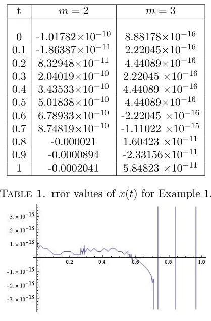
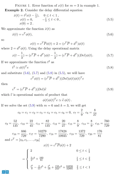
whichIis identity matrix with appropriate dimension. The equation set (14) is solved bym= 2 andm= 3 and the error values in some points is presented in Table 1 and the the error function is plotted in Figure 1 form= 3 . Numerical ﬁndings show the high accuracy of aproximate solution despiteτ =

√ 2 2 .

t m= 2 m= 3

0 -1.01782×10−10 8.88178×10−16 0.1 -1.86387×10−11 2.22045×10−16 0.2 8.32948×10−11 4.44089×10−16 0.3 2.04019×10−10 2.22045×10−16 0.4 3.43533×10−10 4.44089×10−16 0.5 5.01838×10−10 4.44089×10−16 0.6 6.78933×10−10 -2.22045×10−16 0.7 8.74819×10−10 _-1.11022_×₁₀−15

0.8 -0.000021 1.60423×10−11 0.9 -0.0000894 -2.33156×10−11 1 -0.0002041 5.84823×10−11

(13)

Figure 1. Error function of x(t) for m= 3 in example 1.

Example 2. Consider the delay diﬀerential equation

˙

x(t) =t2x(t−1₃), 0≤t <1, x(t) = 0, −1₃ ≤t <0, x(0) = 2.

(5.5)

We approximate the function ˙x(t) as

˙

x(t) =cTϕ(t), (5.6)

so

x(t) =cTP ϕ(t) + 2 = (cTP+dT)ϕ(t) where 2 =dTϕ(t).Using the delay operational matrix

x(t− 1

3) = (c

T_P₊_dT₎_ϕ₍_t₋1

3) = (c

T_P₊_dT₎₍_Del₎_ϕ₍_t₎_. _(5.7)

If we approximate the functiont2 as

t2 ≃ϕ(t)Te (5.8)

and substitute (5.6), (5.7) and (5.8) in (5.5), we will have

cTϕ(t) = (cTP+dT)(Del)ϕ(t)ϕ(t)Te

then

cT = (cTP +dT)(Del)eb (5.9)

whichebis operational matrix of product that

ϕ(t)ϕ(t)Te≃be ϕ(t).

If we solve the set (5.9) withm= 6 and k= 3, we will get

c0 =c1 =c2 =c3 =c4 =c5 =c6 = 0, c7 =

2 9, c8=

8 27

c9 =

52

135, c10= 22

45, c11= 82

135, c12= 20

27, c13= 8

9, c14= 8

9, c15= 760 729

c16=

886

729, c17= 10279

7290 , c18= 17828

10935, c19= 1372

729 , c20= 176

81 andcT = [c0, c1, . . . , c20]

x(t) =cTP ϕ(t) + 2

=           

2 0≤t < 1₃

2 3t

3₊160 81

1 3 ≤t <

2 3

t6

9 − 2 15t5+

t4

18+ 158 243t3+

64856 32805

2

(14)

which is the exact solution.

Example 3. Consider the following delay system with delay in both control and state [13,15]

˙

x(t) +x(t) + 2x(t−₄1) = 2u(t−1₄) 0≤t <1, x(t) =u(t) = 0, −1₄ ≤t≤0,

u(t) = 1, t >0.

(5.10)

The exact solution is [5]

x(t) =                     

0, 0≤t < 1₄,

2−2e−(t−14), 1

4 ≤t < 1 2,

−2−2e−(t−41)+ (2 + 4t)e−(t− 1

2), 1

2 ≤t < 3 4,

6−2e−(t−41)+ (2 + 4t)e−(t− 1 2)−(17

4 + 2t+ 4t2)e−

(t−3₄)_, 3

4 ≤t <1.

Using (5.10) we know

u(t) =   

0, −1₄ ≤t≤0,

1, t >0,

then

u(t−1

4) =   

0, 0≤t≤ 1₄,

1, t > 1₄,

=uTϕ(t)

which the vectoru can be calculated by (3.2). Suppose that

˙

x(t) =cTϕ(t)

so

x(t) =cTP ϕ(t).

wherecis unknown vector. Using the delay operational matrix and (5.10)

cT = 2uT(I+P + 2P(Del))(−1) (5.11)

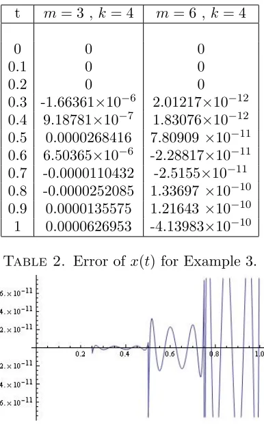
whereI is identity matrix with appropriated dimension. We solve (5.11) with

(15)

t m= 3 , k= 4 m= 6 , k= 4

0 0 0

0.1 0 0

0.2 0 0

0.3 -1.66361×10−6 2.01217×10−12 0.4 9.18781×10−7 1.83076×10−12 0.5 0.0000268416 7.80909×10−11 0.6 6.50365×10−6 -2.28817×10−11 0.7 -0.0000110432 -2.5155×10−11 0.8 -0.0000252085 1.33697×10−10 0.9 0.0000135575 1.21643×10−10 1 0.0000626953 -4.13983×10−10

Table 2. Error ofx(t) for Example 3.

Figure 2. Error function ofx(t) in Example 3 for m= 6 ,k= 4.

Example 4. Consider the delay diﬀerential equation [13] (

˙

x1(t)

˙

x2(t)

) =

(

0 1

−25 −5t

) (

x1(t−1₄)

x2(t−1₄)

) +

( 0 1

)

with ₍

x1(t)

x2(t)

) =

( 0 0

)

,

[ −1

4,0 ]

.

The exact solutions are [8]

x1(t) =

                  

0, 0≤t < 1₄

1 32−

t 4+

t2 2,

1 4 ≤t <

1 2

1 32−

19 96t+

3 16t

2₊5 8t

3₋ 5 12t

4_, 1

2 ≤t < 3 4

−9641 32768+

37391 24576t−

3183 1024t2+

785 256t3−

45 128t4−

85 96t5+

5 18t6,

3

(16)

and

x2(t) =

                  

t, 0≤t <1

4

− 5 384+t+

5 8t

2₋5 3t

3_, 1

4 ≤t < 1 2

775 1536−

17 8t+

1295 192t

2₋115 24t

3₋75 32t

4₊5 3t

5_, 1

2 ≤t < 3 4

3666575 5505024 −

1051 1024t−

95755 49152t

2 +21515

1536t

3₋55325 3072t

4 +335

96t 5

+2125 576t

6₋25 21t

7

, 3

4 ≤t <1. We approximate the function ˙x1(t) and ˙x2(t) as

˙

x1(t) =cTϕ(t), x˙2(t) =uTϕ(t) (5.12)

by initial conditions

x1(t) =cTP ϕ(t), x2(t) =uTP ϕ(t).

Using the delay operational matrix

x1(t−1₄) =cTP ϕ(t−1₄) =cTP(Del)ϕ(t),

x2(t−1₄) =uTP ϕ(t−1₄) =uTP(Del)ϕ(t),

(5.13)

If we approximate the functions

1 =dTϕ(t), t=ϕ(t)Te, (5.14)

and use the operational matrix of productbeand substitute (5.12), (5.13) and (5.14) in main problem, we will have

{

cT ₌_uT_P₍_Del₎_,

uT =−25cTP(Del)−5uTP(Del)eb+dT, (5.15)

whichebis the operational matrix of product

ϕ(t)ϕ(t)Te=be ϕ(t).

Solving (5.15) by N =k= 4 and m= 7 gives the exact values for x1(t) and

x2(t).

6. Conclusions

(17)

polynomial. The illustrative examples demonstrate that the proposed method is valid.

References

[1] M. I. Bhatti and P. Bracken, Solutions of diﬀerential equations in a Bernstein polynomial basis, Journal of Computational and Applied Mathematics, 205, (2007), 272−280. [2] R.Y. Chang, M.L. Wang, Shifted Legendre direct method for variational problems, J.

Optim. Theory Appl. 30, (1983), 299-307.

[3] C.F. Chen, C.H. Hsiao, A Walsh series direct method for solving variational problems, J. Franklin Inst. 300, (1975), 265-280.

[4] H.Y. Chung, Y.Y. Sun, Analysis of time-delay systems using an alternative method, Int. J. Control 46, (1987), 1621-1631.

[5] K.B. Datta, B.M. Mohan, Orthogonal Functions in Systems and Control, World Scien-tiﬁc, Singapore, 1995.

[6] J.S. Gu, W.S. Jiang, The Haar wavelets operational matrix of integration, Int. J. Syst. Sci. 27, (1996), 623-628.

[7] I.R. Horng, J.H. Chou, Shifted Chebyshev direct method for solving variational prob-lems, Int. J. Syst. Sci. 16, (1985), 855-861.

[8] C. Hwang, M.Y. Chen, Analysis of time-delay systems using the Galerkin method, Int. J. Control 44, (1986), 847-866.

[9] C. Hwang, Y.P. Shih, Laguerre series direct method for variational problems, J. Optim. Theory Appl. 39, (1983), 143-149.

[10] M. Jamshidi, C.M.Wang, A computational algorithm for large-scale nonlinear time-delays systems, IEEE Trans. Syst. Man. Cybernetics SMC-14, (1984), 2-9.

[11] K. Maleknejad, Y. Mahmoudi, Numerical solution of linear Fredholm integral equation by using hybrid Taylor and block-pulse functions, Appl. Math. Comput. 149, (2004), 799-806.

[12] H.R. Marzban, H.R. Tabrizidooz, M. Razzaghi, Solution of variational problems via hybrid of block-pulse and Lagrange interpolating, IET Control Theory Appl. 3,(2009), 1363-1369.

[13] H.R. Marzban, M. Razzaghi, Solution of time-varying delay systems by hybrid functions, Math. and Com. in Sim. 64, (2004), 597-607.

[14] H.R. Marzban, M. Razzaghi, Optimal control of linear delay systems via hybrid of block-pulse and Legendre polynomials, J. Franklin Inst. 34, (2004), 279-293.

[15] H.R. Marzban, M. Razzaghi, Analysis of Time-delay Systems via Hybrid of Block-pulse Functions and Taylor Series, J. Vibration and Con. 11, (2005), 1455-1468.

[16] P.N. Paraskevopoulos, P. Sklavounos, and G.CH. Georgiou The operation matrix of integration for Bessel functions, Journal of the Franklin Institute, 327, (1990), 329-341. [17] M. Razzaghi, S. Youseﬁ, The Legendre wavelets operational matrix of integration, Int.

J. Syst. Sci. 32 (4),(2001), 495-502.

[18] M. Razzaghi, S. Youseﬁ, Sine-cosine wavelets operational matrix of integration and its applications in the calculus of variations, Int. J. Syst. Sci. vol. 33, no. 10,(2002), 805-810. [19] M. Razzaghi, M. Razzaghi, Fourier series direct method for variational problems, Int.

J. Control 48, (1988), 887-895.

[20] M. Razzaghi, H.R. Marzban, Direct method for variational problems via hybrid of block-pulse and Chebyshev functions, Math. Probl. Eng. 6, (2000), 85-97.

(18)

[22] X.T. Wang, Numerical solutions of optimal control for time delay systems by hybrid of block-pulse functions and Legendre polynomials, Appl. Math. Comput. 184, (2007), 849-856.

[23] S. A. Youseﬁ, M. Behroozifar, Operational matrices of Bernstein polynomials and their applications, Int. J. Syst. Sci. 41, (2010), 709-716.

[24] S. A. Youseﬁ, M. Behroozifar, Mehdi Dehghan, The operational matrices of Bernstein polynomials for solving the parabolic equation subject to speciﬁcation of mass, Journal of Computational and Applied Mathematics 235, (2011), 5272-5283.